Shital Patil*![]() | Surendra Bhosale
| Surendra Bhosale![]()
© 2023 IIETA. This article is published by IIETA and is licensed under the CC BY 4.0 license (http://creativecommons.org/licenses/by/4.0/).
OPEN ACCESS
Cardiovascular diseases, globally recognized as prominent contributors to morbidity and mortality, have led to an imperative demand for precise, accessible, and efficient diagnostic methodologies. This study introduces a hybrid classification system integrating an ensemble model and a Fuzzy C Means-based neural network with the objective of augmenting predictive accuracy. A comparative analysis on scalar standards was undertaken to determine the optimal feature scaling technique, thereby enhancing predictive proficiency while optimizing time efficiency. The study further incorporates Random Forest, Support Vector Machines, k-Nearest Neighbor, and deep learning models into the diagnostic framework, while employing a confusion matrix as a performance evaluation tool. The GridsearchCV technique is utilized for hyperparameter optimization, its influence on the accuracy of machine learning (ML) models is critically examined. Special attention is given to the role of outliers and their manipulation using supervised ML algorithms, investigating the impact of outlier exclusion on model accuracy. The experimental data was sourced from a cardiovascular patients dataset in the UCI Machine Learning Repository. The findings of the study suggest that the proposed classifier ensemble model surpasses comparable advancements, achieving an exemplary classification accuracy of 98.78%. This paper thus contributes to the evolving landscape of ML application in cardiovascular disease prediction, emphasizing the significance of outlier detection and hyperparameter optimization.
k-Nearest Neighbor, Random Forest, hyper-parameter optimization, Neural Networks, Support Vector Machine, outlier detection
The healthcare sector generates an enormous volume of data pertaining to patients, diseases, and medical evaluations. However, the efficient analysis of this data remains largely untapped, thereby limiting its potential impact on patient health. At the forefront of global mortality causes is heart disease, accounting for an alarming number of fatalities each year. As per the World Health Organisation [1], cardiovascular diseases (CVDs) represent the leading cause of death globally, claiming an estimated 17.9 million lives annually. CVDs encompass a range of conditions such as coronary artery disease, rheumatic heart disease, vascular disease, along with various disorders affecting the heart and blood vessels. Notably, strokes and heart attacks constitute four out of every five CVD deaths [2].
A multitude of risk factors contribute to heart disease, including sex, smoking habits, age, family medical history, poor diet, high cholesterol, physical inactivity, high blood pressure, obesity, and alcohol consumption. Inherited risk factors encompass conditions such as diabetes and high blood pressure [3]. Secondary factors, such as physical inactivity, obesity, and unhealthy diets, further amplify this risk. Typical signs and symptoms include generalized weakness, fatigue, palpitations, excessive sweating, back pain, chest pain, discomfort in the shoulder and arm, and shortness of breath. Chest pain, medically referred to as angina [4], remains the most common symptom of insufficient blood flow to the heart. Diagnostic tests such as X-rays, MRI scans, and angiography are employed to confirm the diagnosis.
However, instances arise where an inadequacy of medical equipment leads to a resource deficit during emergencies. The urgency of diagnosing and treating cardiovascular disease cannot be overstated, as every second is of the essence. Cardiac centers and outpatient clinics generate voluminous data concerning heart disease detection, highlighting a significant potential need for enhanced big data analytics in the context of cardiovascular care and patient outcomes [4, 5].
Yet, the task of deriving precise, accurate, and valid conclusions is often impeded by disturbances, inconsistencies, and variability in the data. With the advent of significant technological advancements in big data, knowledge storage, acquisition, and recovery, artificial intelligence (AI) has become crucial in the field of cardiology [6]. Multiple machine learning (ML) models have been employed by researchers to make decisions, following the pre-processing of data using various data mining techniques [7]. A broad spectrum of ML algorithms and variants are utilized in monitoring hereditary cardiac disorders and control, aiming to forecast the early stages of heart failure [8]. A host of heart attack prediction algorithms, including KNN, DT, SVC, LR, and RF machine algorithms, have been explored [9, 10].
Unsupervised ML: data-driven, unlabelled data (clustering); Supervised ML: task-driven, labelled data (classification/regression); among the three kinds of machine learning approaches is reinforcement learning, which involves learning from failures while engaging in games [11]. In this study, supervised machine learning (ML) classifiers including Logistic Regression (LR), k-Nearest Neighbours (kNN), Support Vector Machine (SVM), and others are used to demonstrate how various models may predict the presence of heart disease and to compare the accuracy of these classifiers. Neural Network (NN), Decision Tree (DT), Random Forest (RF), FCC Means – SVM, FCC Means – NN, KNN Means – SVM and KNN Means – NN. The remainder of the paper is organized as follows: The literature review is found in Section 2. Section 3 discusses the recommended technique. Section 4 discusses the experiment's findings. To summarise, Section 5 contains the conclusions.
The literature survey shows insightful information about feature extraction methods as discussed. In fact, hybrid intelligent systems that integrate the benefits of neural Networks with fuzzy systems can do quite well when handling challenging issues. Neural Networks are powerful tools for learning patterns and extracting features from data, while fuzzy systems handle uncertainty and make decisions based on imprecise information. By integrating these two approaches, hybrid intelligent systems can leverage the learning capabilities of Neural Networks to model complex relationships and extract knowledge from large datasets. The fuzzy systems can then use this learned knowledge to make decisions and handle uncertainty, providing a more robust and flexible solution [11, 12]. One common approach to building hybrid intelligent systems is to use Neural Networks for feature extraction and pattern recognition. The neural network can be trained on a large dataset to learn the underlying patterns and extract relevant features. Overall, hybrid intelligent systems that integrate Neural Networks and fuzzy systems can leverage the strengths of both approaches, offering excellent performance in solving complex problems, particularly in scenarios where learning from data and handling uncertainty are crucial, resulting in a hybrid combination for achieving good results [13].
The author suggested creating an algorithm that may predict a cardiac illness's propensity based on basic symptoms including age, gender, pulse rate, and other factors. The recommended solution uses the Neural Network machine learning approach since it has been shown to be the most reliable and accurate algorithm [14].
This approach uses a consensus clustering algorithm to cluster the instances in the majority class. Consensus clustering is a technique that combines multiple clustering results to obtain a more robust and reliable clustering solution. It helps to reduce the impact of noise and variations in the data [15]. By using this approach, the majority class's instance count is really decreased. addressing the issue of class imbalance. As a result, machine learning models may perform better, particularly when there is a significant class divide and the majority class exceeds the minority class. In terms of prediction performance, The ensemble word embedding scheme performs better than the other schemes, according to an empirical investigation [16].
The article [17] presents a comprehensive comparison of the feature engineering schemes and base learners. This study investigates four distinct categories of features, used in Random Forest, including authorship attribution characteristics, character n-grams, part of speech n-grams, and the frequency of the most discriminative terms.
Overall, the study aims to compare algorithms, fine-tune hyperparameters using GridsearchCV, and improve the accuracy of algorithmic models for predicting heart problems. Using validated data splitting and appropriate performance metrics will ensure reliable and meaningful results in healthcare systems [18].
Problem Statement: Analysis of various traditional ML algorithms and their ensemble approaches were adopted for detecting cardiac diseases. Moreover, enhancing classification rate from optimization algorithms with hyperparameter-based tuning algorithm and grid search CV method. This paper uses the shorter population of critical medical data for a relatively smaller set of patients as the large dataset is recommended for such analytical studies. In order to address such practical constraints, it envisages exploring to compare the performance of each of the traditional models in regard to its counterpart in an attempt to choose an optimized model. The effect of hyper-tuning of the metric parameters on accuracy improvement shall be the point of interest. Also, possible outliers must be detected and processed to evaluate the prediction accuracy of these models [19]. Analysis of various traditional ML algorithms and their ensemble approaches were adopted for detecting cardiac diseases. Moreover, enhancing the classification rate of optimization algorithms with a hyper-parameter-based tuning algorithm and grid search CV method.
This research study discusses the use of traditional machine learning algorithms and their ensemble approaches for detecting cardiac diseases as an attempt to choose the best possible existing algorithms fit for such critical applications in medical science. The study uses a relatively smaller population dataset from the UCI Machine Learning Repository, which represents a challenge to AI/ML community and considered only fourteen important attributes for the proposed model in consultation with experts. Data cleaning was not availed as it is pre-processed dataset. Feature scaling was done using three scaling datasets, and the best accuracy was obtained from the standard scalar. Data splitting was done to train and test SVM, RF, and NN models [20]. The performance was analyzed for different split ratios, and the 70:30 split ratio was used for further experimentation to validate the data-splitting practice for critical medical applications. Data visualization was done using a histogram, which helped to identify the attributes that have a higher correlation with heart disease through analysis.
The novelty in this paper appears to be the proposed method for detecting cardiac diseases using various traditional machine learning algorithms and their ensemble approaches [21], as well as enhancing the classification rate through optimization algorithms with hyper-parameter-based tuning algorithm and grid search CV method. The authors also conducted experiments on a pre-processed dataset and evaluated the performance of different scaling techniques and data-splitting ratios. The data visualization and analysis of different attributes of the dataset for predicting and validating the proposed model is also a novel aspect of this text.
The objective of this paper is to explore feature selection techniques and it also emphasizes analyzing the behavior of the used model in the presence of an outlier in the smaller dataset which poses a challenge to the ML community. Cardiac disorder being a very critical application to human life, an outlier in the dataset must be included in practice time, and evaluating model performance in such a scenario proves to be useful to physicians.
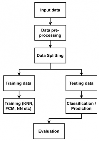
This work performs a comparative study with the feature selection techniques. One can conclude and see which type of feature selection technique works relatively better if the model is random forest-based or ANN based or SVM based. Although the paper does not touch upon any information about the architecture of the models, this model is accurately used for comparing the feature selection techniques for better performance in the context of smaller datasets as an attempt to come up with a recommendation to the physician for selecting specific physiological attributes. The approach can be run in a pipeline wherein the physician can recommend a few corrective measures in selecting the attribute to see performance analytics. The proposed method is depicted in Figure 1.
Figure 1. Proposed method block diagram
3.1 Details of dataset
The proposed method has been evaluated and validated on UCI Machine Learning Repository datasets. It consists of 76 attributes. For experimentation purposes, we considered only 14 attributes for the significance of the proposed model. Some attributes give the same knowledge while other attributes are not relevant to the targeted attribute. Thus, redundant attribute data have been discarded from the data. Only relevant and discriminating attributes are taken into consideration. Table 1 provides a detailed description of data attributes used to predict and validate the proposed model.
3.2 Splitting and pre-processing of data
$\frac{X_{\text {scaled }}=X-X_{\min }}{X_{\max }-X_{\min }}$ (1)
where X indicates feature, Xmin, Xmax, and Xscaled refer to the minimum, maximum, and scaled feature values respectively. Table 1 lists the details of the attributes pertaining to the heart dataset.
Table 1. Heart dataset attribute information
|
Data Attributes |
Description |
|
Sex |
Gender, 0 = Female, 1=Male |
|
Age |
Age (years) |
|
Chest Pain (Cp) |
Chest pain Types (3: Asymptomatic, 2: Non-angina, 1: Atypical angina, 0: typical angina.) |
|
Chol |
Serum cholesterol in mg/d |
|
Tresbps |
Blood Pressure calculated at rest position (in mm Hg on admission to the hospital) |
|
Ca |
Major vessels (0-3) coloured by fluoroscopy |
|
FBS |
Fasting blood sugar >120 mg/dl), (0 = false, 1 = true) 1. Resting electrocardiographic results 2: probable or definite left |
|
Restecg |
ventricular hypertrophy by Estes criteria, 1: ST-T wave abnormality, 0: normal) |
|
Exang Thalach |
Exercise-induced angina (0 = no, 1 = yes) Maximum heart rate achieved |
|
Oldpeak |
ST depression induced by exercise relative to rest |
|
Thal |
7 = reversible defect; 6 = fixed defect; 3 = normal |
|
Slope |
Peak exercise Slope (2: down sloping, 1: flat, 0: up sloping) |
|
Num |
1: Unhealthy, 0: Healthy |
Table 2 indicates the best accuracy obtained from the standard scalar. Hence, the standard scalar is applied for further feature scaling in the experimentation. The Standard Scalar scales the data at zero mean and unit SD by assuming the data is normally distributed within each feature.
Table 2. Comparison of the three scalers' performance in terms of accuracy (%)
|
Scalar |
SLRstd |
SLRmm |
SLRr |
|
ACC (%) |
86.78 |
84.90 |
85.84 |
For any model, maximum training data makes the system robust. The 50:50 data for training and testing is not a good choice for less data. The in present study, the four different ratios were selected to train, test SVM, RF, and NN, and noted the performance in every case. Table 3, indicates the analysis of training ACC (%) for different split ratios. It was noted that the 70:30 split provide des highest ACC. Hence, the 70:30 split ratio is used for further experimentation [24].
Table 3. Performance of SVM, NN, RF for different split ratios in terms of accuracy (%)
|
Algorithm |
60:40 |
70:30 |
75:25 |
80:20 |
|
RF |
86.74 |
92.45 |
90.31 |
85.12 |
|
NN |
84.53 |
84.91 |
84.14 |
82.64 |
|
SVM |
86.70 |
86.79 |
85.02 |
84.30 |
3.3 Visualization of data
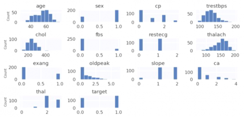
Data Visualization provides more insights into the evaluation process hence readers engage and interact more closely with new findings. It shows an easier way to communicate the research in the community. Figure 2 shows a graphical representation f the present dataset for good understanding. In the histogram, the plot y-axis represents the count of the respective attributes whereas different attributes of the dataset have shown on the x-axis.
The distribution of heart disease patients with various attributes is presented in Table 1 viz. sex, age, Cp, etc. It’s clearly noted from the plots which attributes are belonging categorical numerical variables. Interpretation from histogram plots is discussed below [24].
Figure 2. Histogram showing different attributes of heart patients
3.4 ML models for prediction of cardiac disorders
3.4.1 Support vector machine
It is a linear classifier. The two-class separating hyper-plane is selected to optimize desired classification error for unknown test data. SVM is a binary classification model. SVM classifies the test data point to the class nearest point in the training data. Non-linear and non-separable data is transferred to higher dimension feature space and separated by a hyperplane. The process of mapping to higher-dimension feature space is performed by using different kernels. SVM provides [6] give the best two-class separating hyperplane that maximizes the separating distance.
$y=w x+b$ (2)
3.4.2 Neural Networks (NN)
It simulates the system which can take decisions like human brain. ANN has ability to learn and realize various study patterns to obtain information. This creates a link between input neuron to output neuron. Neurons are functions of weighing factors. The output can be measured by taking product of specific neuron weight with input. Afterword, it compared with threshold value. The result is greater than given threshold value. It is considered as output. Practically, it is impossible to evaluate how many layers or nodes to be utilized in ANN to address a specific application. It has to evaluate by systematic experimentation to find best for the given data. Thus, after using various values of hidden layers, best suitable results were noted with 100 hidden layers [25].
3.4.3 Random Forest (RF)
RF works on the principle of decision trees at training. Predictions of different trees are pooled to find final prediction. The feature importance of decision tree can be evaluated as,
$F i_i=\frac{\sum_{j=n o d e s}^n n i_i}{\sum_{k=1}^n n i_k}$ (3)
where Fii is feature importance, node j has importance nij. The mean of all the trees provides the final feature importance value. It can be calculated by sum of the feature’s important value of each tree, divided by the value of total trees [6].
$R F f i_i=\frac{\sum_{j \in t r e e s}^n n o r m f i_{i j}}{T}$ (4)
where, RFfii denotes feature importance when evaluated from all trees in the RF model, norm fiij. Indicates the normalized feature importance for i in the tree.
3.4.4 K-Nearest Neighbors
It is a simple ML algorithm. It works on the principle of majority votes of neighbors to classify the unknown object. When the unknown sample is provided, the cluster area for k training samples, which are close to unknown samples, is searched by KNN algorithm. Euclidean distance between two given points Y = (y1, y2. . . ym) and X = (x1, x2 ... xm) can be given by,
$d(x, y)=\sqrt{\sum_{i=1}^m\left(x_i-y_i\right)^2}$ (5)
3.4.5 K-Means-based SVM
The prediction analysis of this model has two stages. Initially, the k-mean clustering has employed which clusters hybrid datasets. Finally, the SVM model has been employed that will classify the data.
3.4.6 K-Means based Neural Network
The performance of classification analysis model has two phases. Firstly, k-mean clustering has evaluated on data that results in cluster dissimilar and similar type of data. Afterwards, the NN model has employed to separate data types. Here, the first step will be same as K means based SVM.
3.4.7 Fuzzy C-Means based Neural Network
It is a soft clustering method. It allows partial belongings of pixels in various clusters. So as to addition of all degrees is 1 for any data types. This method is applicable to segmentation applications compared to hard clustering algorithms. This model evaluates ‘c’ clusters by optimizing the objective function defined as,
$J_{F C M}=\sum_{k=1}^n \sum_{i=1}^c\left(u_a\right)^q d^2\left(x_k, v_i\right)$ (6)
where, data points are denoted by xk = x1, x2 ... xn, the data items are indicated by n, c provides clusters count, the membership degree of xk in the ith cluster is denoted as uik, weighting exponent of membership is shown by q, vi is cluster center, d2(xk, vi) The distance in cluster center v and data point xk is denoted by d. In the proposed hybrid model, the output of Fuzzy C-means has been provided as input to the NN for best classification. Maximum accuracy is obtained from the fuzzy c-partitioned matrix. It is noted that the accuracy is improved by implementing this Hybrid method compared to only Neural Network.
3.4.8 Fuzzy C-Means based SVM
This algorithm is implemented as per the following steps:
To begin, the Fuzzy C model is applied to the provided dataset. Following that, a Fuzzy c-partitioned matrix is evaluated.
As input to the SVM method for classification, a combination of Fuzzy partition matrix and feature set is already available.
It has been discovered that when the Hybrid approach is used, classification accuracy improves when compared to using solely SVM.
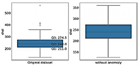
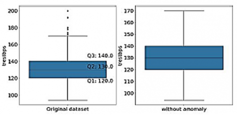
The results shown in Table 4 are based on the dataset, which has anomalies in it. To see the effect of removal of outliers, outlier detection has been computed [16]. Anomaly detection was performed on all the parameters using boxplots. Boxplots the for original dataset (with outliers) and clean dataset (without outliers) for numerical fields have been shown in Figures 3-7.
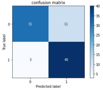
4.1 Confusion matrix-based analytics
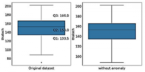
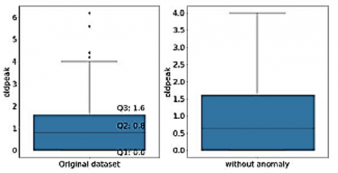
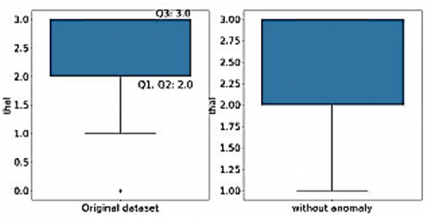
Figures 3-7 shows the box plot of chol, trestbps, thalach, old peak and thal attributes before and after removal of outliers respectively. Boxplot graphically representation of two or more numerical datasets by their quartiles. The lines extending from the boxes represent the variations in lower and upper quartiles. Outliers are the points ranging outside a specific range. Q1 represents 25 percentiles, Q3 represents 75 percentile, and Inter Quartile Range (IQR) is given by (Q3-Q1). Data points which are less than Q1 − 1.5 ∗ (IQR) and greater than Q3 + 1.5 ∗ (IQR) are mentioned as outliers. For Chol attribute, Q1 is 211 and Q3 is 274.5, while the lower bound is 115.75 and upper bound is 369.75. So, the points below lower bound and greater than upper bound are shown as outliers. For Chol, there are no points below the lower bound, but there are 5 points above the upper bound (shown in left subplot). These outliers have been filtered out as shown in right subplot. For trestbps attribute, Q1 is 120 and Q3 is 140 while the lower bound is 90 and up-per bound is 170. So, the points below lower bound and greater than upper bound are shown as outliers. For trestbps, there are no points below the lower bound, but there are 9 points above the upper bound (shown in left subplot). These outliers have been filtered out as shown in right subplot. Figures 3-6 indicates the box plot before and after removal of anamolies respectively for dataset parameters namely “chol”, “trestps”, “thalach”,”old peak” and “thal”. Confusion matrix-based analytics is used in this paper for better understanding of relative performance. For Thalach attribute, Q1 is 133.5 and Q3 is 166 while the lower bound is 84.75 and upper bound is 214.75. So, the points below lower bound and greater than upper bound are shown as outliers. For this attribute, there are no points above the upper bound, but there is 1 point below the lower bound (shown in left subplot). These outliers have been filtered out as shown in right subplot. For oldpeak attribute, Q1 is 0 and Q3 is 1.6 while the lower bound is -2.4 and upper bound is 4. So, the points below lower bound and greater than upper bound are shown as outliers. For this attribute, there are no points below the lower bound, but there are 5 points above the upper bound (shown in left subplot). These outliers have been filtered out as shown in right subplot. For Thal attribute, Q1 is 2 and Q3 is 3 while the lower bound is 0.5 and upper bound is 4.5. So, the points below lower bound and greater than upper bound are shown as outliers. For this attribute, there are no points above the upper bound, but there are 2 points below the lower bound (shown in left subplot). These outliers have been filtered out as shown in the right subplot.
Table 4. Accuracy of various models prior to tuning
|
ML Model |
ACC (Testing) |
ACC (Training) |
|
KNN |
82.42 |
84.91 |
|
SVM |
80.22 |
86.22 |
|
NN |
82.41 |
90.21 |
|
RF |
75.82 |
90.21 |
|
FCC Means – SVM |
86.89 |
87.60 |
|
FCC Means – NN |
88.52 |
95.04 |
|
KNN Means – SVM |
84.62 |
80.06 |
|
KNN Means - NN |
83.52 |
91.98 |
Figure 3. Box plot of “chol” attribute before and after removal of anomalies
Figure 4. Box plot of “trestbps” attribute before and after removal of anomalies
Figure 5. Box plot of “thalach” attribute before and after removal of anomalies
Figure 6. Box plot of “old peak” attribute before and after removal of anomalies
Table 5. Methods of dealing with missing values
|
Feature Name |
Number of Rows Dropped |
Interpolated Average |
|
Chol |
5 |
243 |
|
Trestbps |
9 |
130 |
|
Thalach |
1 |
150 |
|
Oldpeak |
5 |
0.9 |
|
Thal |
2 |
2 |
Figure 7. Box plot of “thal” attribute before and after removal of anomalies
Figure 8. Confusion matrix for SVM
Figure 9. Confusion matrix for Neural Network
Figure 10. Confusion matrix for Random Forest
Figures 8-10 show confusion matrix for the models like SVM, Neural Network, and Random Forest, respectively.
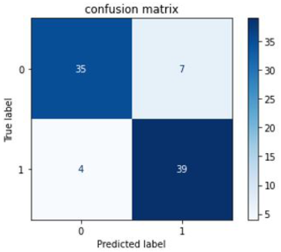
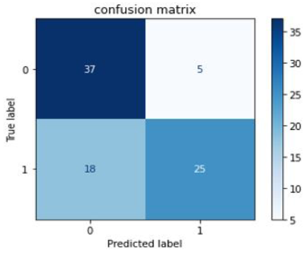
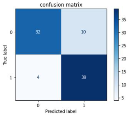
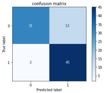
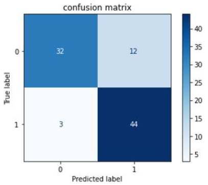
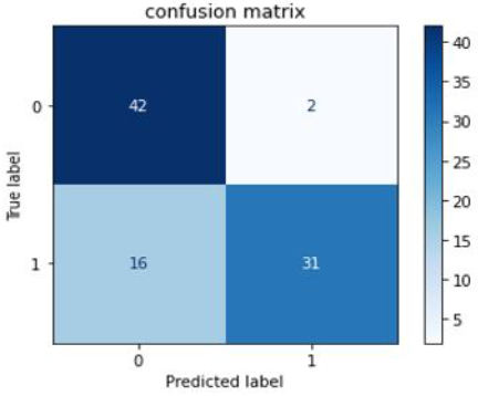
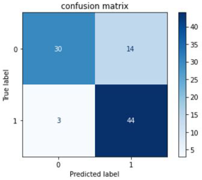
After the outlier detection, we are left with two options. Either drop the rows since they contain an outlier or. Fill these outlier gaps in an appropriate way. In this work, we have tried both ways to check which method may be better. Here interpolation has been done using the average value of the respective feature. These scopes have been shown in Table 5, columns 2 and 3. Once the outliers have been detected and further processing of outliers has been done. The processed datasets have been put into 4 classification algorithms to check their performance. Based on the results in Table 4, the hybrid models outperform the simple method, we decided to check the dataset after removal of outliers using simple methods. If the accuracies improve after outlier removal, it is assumed that the hybrid models will definitely perform better. Figures 11-15 depicts the confusion matrix for SVM, KNN, Neural Network, Random Forest, and KNN respectively.
Figure 11. Confusion matrix for SVM
Figure 12. Confusion matrix for KNN
Figure 13. Confusion matrix for Neural Network
Figure 14. Confusion matrix for Random Forest
Figure 15. Confusion matrix for KNN
4.1.1 Dropping missing values after removal of outliers
After dropping 21 rows, we are left with 282 rows. To check the efficiency of the removal of outliers (by dropping them), we have tested the dataset with 4 classification algorithms. The 4 Classification algorithms are SVM, Neural Network, Random Forest, and KNN (as shown in Table 5). For each of the classification algorithms, the confusion matrix has been shown.
4.1.2 Interpolating the values by their respective Average value after outlier detection
Instead of dropping the rows containing the outliers, we have deleted those outliers and filled those missing values by the average values of the feature.
In this way, there has been no loss of data (especially those 21 rows which were dropped in 1st case).
This processed dataset was again applied to all 4 classification algorithms and its confusion matrix has been created.
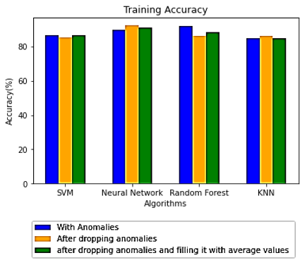
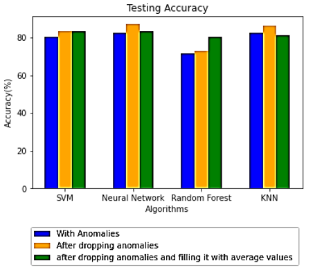
For all 4 algorithms, the accuracy after deleting the rows
(Yellow bar) containing outliers have improved compared to results with anomalies. While in 2 cases, interpolated accuracies have been equal to or greater than the accuracies received after dropping the rows containing the outliers. Confusion matrix-based analytics is shown in Figures 8-15 for various methods of analysis.
4.2 Methods for data optimization
There are various ways for data optimization to employ the model.
Figure 16. Comparison of classification training accuracy for different algorithms
Figure 17. Comparison of classification testing accuracy for different algorithms
1. Imputation of Data: Missing values in a dataset can pose challenges when training machine learning models. Many models are unable to handle missing values directly, as they require complete data for training. To address missing values, an imputation technique can be used to fill in or estimate the missing values based on the available data.
Table 6. Prediction accuracy of all models after employing GridsearchCV
|
ML Model |
ACC (Testing) |
ACC (Training) |
|
KNN |
83.54 |
87.26 |
|
SVM |
83.52 |
86.32 |
|
NN |
83.52 |
93.87 |
|
RF |
77.24 |
86.32 |
|
FCC Means – SVM |
86.89 |
98.78 |
|
FCC Means – NN |
88.52 |
87.19 |
|
KNN Means – SVM |
84.62 |
80.06 |
|
KNN Means - NN |
83.52 |
93.40 |
Comparison of various algorithms like SVN, Neural Networks, Random Forest, KNN, etc during the classification process for training and testing has been analyzed and shown in Figure 16 for training and Figure 17 for testing. Table 6 shows the accuracy of the various models prior to tuning. Prediction of missing values using ML Algorithm.
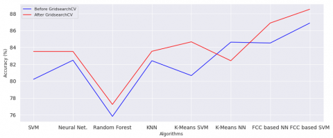
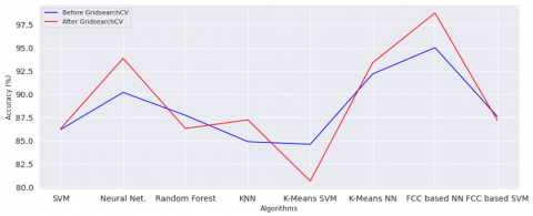
Figure 18. For Comparison of Training Accuracy before and after implementing GridsearchCV
Figure 19. For Comparison of Testing Accuracy before and after implementing GridsearchCV
Furthermore, the choice between regression, classification, or feature-based imputation depends on the specific characteristics of the dataset and the nature of the missing data. It's advisable to experiment with different approaches and evaluate their effectiveness in imputing missing values in order to achieve accurate and reliable results.
2. Categorical Values Handling: When working with categorical values in machine learning models, it is often necessary to transform them into numerical values. This transformation is required because many machine learning algorithms operate on numerical data and cannot directly handle categorical variables. To convert categorical values into numerical representations, encoders are commonly used. Encoders assign a unique numerical value to each category in the categorical variable, establishing a one-to-one mapping between the textual values and their corresponding numerical representations.
3. Data Standardization: Data standardization, also known as normalization, is a common pre-processing step in machine learning to bring the features of a dataset to a similar scale. The Z-score method also referred to as standardization, is one popular technique for achieving this. The Z-score method involves transforming each value of a feature by subtracting the mean of the feature and dividing it by its standard deviation. The formula for standardizing a value x using the Z-score method is shown in the following equation:
$z=(x-\mu) / \sigma$ (7)
where:
z is the standardized value (Z-score),
x is the original value of the feature,
μ is the mean of the feature,
σ is the standard deviation of the feature.
4. Using optimized ML algorithms: It suggests selecting the best hyperparameters required for various models. The classification accuracy of the FCM-based neural network improved to 98.78% after a thorough search of hyperparameters using GridsearchCV. The performance of clustering approaches combined with neural networks, SVM, and statistical classifiers has been compared in Table 7. It has been reported that hybrid models outperformed classical models.
Table 7. Comparison of classifiers for heart disease diagnosis
|
Author |
Year |
Methods/Classifiers |
Datasets |
Evaluation Parameters |
Highest Accuracy% |
|
[26] |
2021 |
SVM, NB, DT |
Heart Dataset (UCI repository) |
Accuracy |
DT 90% |
|
[27] |
2021 |
NB, LM, LR, DT, RF, SVM, HRFLM |
Heart Cleveland (UCI repository) |
Accuracy, Precision, Specificity, Sensitivity, F‐Measure |
HRFLM 88.4% |
|
[28] |
2022 |
LR, Evimp functions, Multivariate adaptive regression |
DiScRi dataset |
Accuracy, Sensitivity, Specificity |
94.09% |
|
[29] |
2022 |
KNN, DT, LR, NB, SVM |
Heart Dataset (UCI repository) |
Accuracy, Specificity, Sensitivity, F1‐Score |
LR 92% |
|
[30] |
2022 |
K‐NN, DT, RF, MLP, NB, L‐SVM, |
IoT based Produced Data |
Accuracy |
L‐SVM 92.30%, RF 92.30% |
|
[31] |
2022 |
DT, NB, KNN, RF, ANN, Ada, GBA |
Heart Disease (Kaggle) |
Accuracy, Precision, recall, f1‐score |
RF 86.89% |
|
[32] |
2022 |
LR, SVM, NB, RF, XGB, DT, NN, RBF, KNN, GBT, MLP |
Heart Disease (UCI Repository) |
Accuracy, Precision (specificity), Recall (sensitivity), F‐Measure |
RF 96.28% |
|
Proposed Methodology |
2023 |
LR, SVM, RF, DT, NN, KNN, Fuzzy C means-based neural network |
Heart Disease (UCI Repository) |
Accuracy, Precision, Recall, F1‐score, MCV |
98.78% |
4.2.1 GridsearchCV
It provides the optimal hyper-parameters to use an algorithm. It has included in the sklears model selection package. It provides the platform for predefined hyper-parameters and it fits the model on a given training dataset. Thus, we can select the best parameters with cross-validation number for individual sets of hyper-parameters. In the proposed study, GridsearchCV is employed in eight different models, to get the best suitable hyper-parameters values. By using new hyper-parameter values, eight ML algorithms have been trained and tested. Hence, there is improvement in prediction accuracy for all eight models has been noted. This has been specified in Table 5 and Figure 18 for evaluating the training accuracy between the two employing GridsearchCV and Figure 19 indicates the accuracy of testing before and after using GridsearchCV method.
The current study's goal is to diagnose heart disease using various ML algorithms and compare them to hybrid models. The hybrid models like the Fuzzy C-means clustering-based neural network and K Means Neural network performed better for training classification accuracy. K Means Neural Network obtained a prediction accuracy of 91.98%, which is enhanced in Fuzzy C-Means to Neural Network with 95.05% without hyperparameter tuning. The classification accuracy increased to 98.78% after a systematic search of hyperparameters with GridsearchCV. for the FCM-based neural network. Performances of the combination of clustering techniques with Neural networks and SVM and statistical classifiers have been compared. It was reported that the hybrid models performed better compared to the classical model. Afterward, the training testing accuracy by removing outliers and thereafter interpolating the rows have been implemented to evaluate the impact of outlier removal. It is discovered that the proposed strategy outperforms the dataset with anomalies. Hence, outlier removal can be recommended for the accurate detection of cardiac disorders. As per the suggestions of cardio, thoracic surgeon, and cardiologist, still there is more scope to work on physiological data like thyroid values, cardiac risk elements, parameters belonging to the clinical background of the family etc. with real-time application of more than 5000 patients. This large dataset can be optimized to have zero classification rate of prediction of cardiac disorders. Hyperparameter tuning is indeed an important aspect of machine learning model development, especially when working with large and diverse datasets. The performance of a model depends not only on the chosen algorithm but also on the values assigned to the hyperparameters, which are the settings that control the learning process. Hyperparameter tuning involves systematically searching for the optimal combination of hyperparameter values that results in the best model performance. This can be done using various techniques such as grid search, random search, Bayesian optimization, or genetic algorithms.
This work is not supported fully or partially by any funding organization or agency.
The authors declare that there is no conflict of interest regarding the publication of this paper.
[1] World Health Organization. Cardiovascular Diseases (CVDs). https://www.who.int/health-topics/ cardiovascular-diseases/#tab=tab_1, accessed on Jan. 10, 2022.
[2] Staff M.C. (2022). Strategies to prevent heart disease. https://www.mayoclinic.org/diseases conditions/heart-disease/indepth/heartdisease- prevention/art-20046502
[3] https://www.heart.org/en/health-topics/high-blood-pressure/why-high-blood-pressure-is-a-silent-killer/ know-your-risk-factors-for-high-blood-pressure, accessed on Jan. 10 2022.
[4] Balla, C., Pavasini, R., Ferrari, R. (2018). Treatment of Angina: Where Are We? Cardiology, 140, 52-67. https://doi.org/10.1159/000487936
[5] Rumsfeld, J.S., Joynt, K.E., Maddox, T.M. (2016). Big data analytics to improve cardiovascular care: Promise and challenges. Nature Reviews. Cardiology, 13(6): 350-359. https://doi.org/10.1038/nrcardio.2016.42
[6] Johnson, K.W., Torres Soto, J., Glicksberg, B.S., Shameer, K., Miotto, R., Ali, M., Ashley, E., Dudley, J.T. (2018). Artificial intelligence in cardiology. Journal of the American College of Cardiology, 71(23): 2668-2679. https://doi.org/10.1016/j.jacc.2018.03.521
[7] Nasrabadi A., Haddadnia J. (2016). Predicting heart attacks in patients using artificial intelligence methods. Modern Applied Science, 10(3): 66. http://dx.doi.org/10.5539/mas.v10n3p66
[8] Alom, Z., Azim, M.A., Aung, Z., Khushi, M., Car, J., Moni, M.A. (2021). Early stage detection of heart failure using machine learning techniques. In Proceedings of the International Conference on Big Data, IoT, and Machine Learning, Cox’s Bazar, Bangladesh, pp. 75-88. http://dx.doi.org/10.1007/978-981-16-6636-0_7
[9] Ramalingam V., Dandapath A., Raja M.K. (2018). Heart disease prediction using machine learning techniques: A survey. International Journal of Engineering Technology, 7: 684-687. https://doi.org/10.14419/IJET.V7I2.8.10557
[10] Zriqat I. A., Altamimi A.M., Azzeh M., (2017). A comparative study for predicting heart diseases using data mining classification methods. https://doi.org/10.48550/arXiv.1704.02799
[11] Aljanabi M., Qutqut H., Hijjawi M., (2018). Machine learning classification techniques for heart disease prediction: A review. International Journal of Engineering Technology, 7(4): 5373-5379. http://dx.doi.org/10.14419/ijet.v7i4.28646
[12] Gavhane A., Kokkula G., Pandya I., Devadkar K. (2018). Prediction of heart disease using machine learning. Second International Conference on Electronics, Communication and Aerospace Technology (ICECA), IEEE, Coimbatore, India, pp. 1275-1278. https://doi.org/10.1109/ICECA.2018.8474922
[13] Khourdifi Y., Bahaj M. (2019). Heart disease prediction and classification using machine learning algorithms optimized by particle swarm optimization and ant colony optimization. International Journal of Intelligent Engineering and Systems, 12(1): 242-252. http://dx.doi.org/10.22266/ijies2019.0228.24
[14] Patil P.M., Deshmukh M. P., Mahajan P. (2005). A novel fuzzy clustering neural network. IEEE International Joint Conference on Neural Networks, 3: 1989-1994. https://doi.org/10.1109/IJCNN.2005.1556185
[15] Asvinth A.M.H. (2000). A computational model for prediction of heart disease based on logistic regression with gridsearchcv. International Journal of Scientific Technology Research, 9, 2020. https://www.ijstr.org/final-print/mar2020/A-Computational-Model-For-Prediction-Of-Heart-Disease-Based-On-Logistic-Regression-With-Gridsearchcv.pdf.
[16] Guzm´an J. C., Miramontes I., Melin P., Prado-rechiga G. (2019). Optimal genetic design of type-1 and interval type-2 fuzzy systems for blood pressure evel classification,’ Axioms, 8(1): 8. https://doi.org/10.3390/axioms8010008
[17] Ramirez E., Melin P., Prado-Arechiga G. (2019). Hybrid model based on neural networks, type-1 and type-2 fuzzy systems for 2-lead cardiac arrhythmia classification. Expert Systems with Applications, 126: 295-307. https://doi.org/10.1016/j.eswa.2019.02.035
[18] Miramontes I., Guzman J.C., Melin P., Prado-Arechiga G. (2018). Optimal design of interval type-2 fuzzy heart rate level classification systems using the bird swarm algorithm. Algorithms, 11(12): 206. https://doi.org/10.3390/a11120206
[19] Melin P., Miramontes I., Prado-Arechiga G. (2018). A hybrid model based on modular neural networks and fuzzy systems for classification of blood pressure and hypertension risk diagnosis. Expert Systems with Applications, 107: 146-164. https://doi.org/10.1016/j.eswa.2018.04.023
[20] J. S. K., S. G. (2019). Prediction of heart disease using machine learning algorithms. 1st International Conference on Innovations in Information and Communication Technology (ICIICT), Chennai, India, pp. 1-5. https://doi.org/10.1109/ICIICT1.2019.8741465
[21] Patil, S., Bhosale, S. (2021). Hyperparameter Tuning Based Performance Analysis of Machine Learning Approaches for Prediction of Cardiac Complications, Proceedings of the 12th International Conference on Soft Computing and Pattern Recognition (SoCPaR 2020). Advances in Intelligent Systems and Computing, vol 1383, Springer.
[22] Onan, A. (2022). Bidirectional convolutional recurrent neural network architecture with group-wise enhancement mechanism for text sentiment classification. Journal of King Saud University - Computer and Information Sciences, 34(5): 2098-2117. https://doi.org/10.1016/j.jksuci.2022.02.025
[23] Patil, S., Bhosale, S. (2022). Assessing feature selection techniques for machine learning models using cardiac dataset. 2022 IEEE Fifth International Conference on Artificial Intelligence and Knowledge Engineering (AIKE), Laguna Hills, CA, USA, pp. 126-130.
[24] Onan, A. (2019). Two-stage topic extraction model for bibliometric data analysis based on word embeddings and clustering. IEEE Access, 7: 145614-145633. https://doi.org/10.1109/ACCESS.2019.2945911
[25] Patil, S., Bhosale, S. (2023). Enhancing heart disease prediction through ensemble learning and feature selection. Computer Integrated Manufacturing Systems, 29(4): 288-296.
[26] Abdalrada, A.S., Abawajy, J., Al-Quraishi, T., Islam, S.M.S. (2022). Machine learning models for prediction of co-occurrence of diabetes and cardiovascular diseases: A retrospective cohort study. Journal of Diabetes and Metabolic Disorders, 21: 251-261. https://doi.org/10.1007/s40200-021-00968-z
[27] Kishor, A., Jeberson, W. (2020). Diagnosis of heart disease using internet of things and machine learning algorithms. In Proceedings of the Second International Conference on Computing, Communications, and Cyber-Security, Ghaziabad, India, pp. 691-702.
[28] Kondababu, A., Siddhartha, V., Kumar, B.B., Penumutchi, B. (2021). A comparative study on machine learning based heart disease prediction. Materials Today: Proceedings. https://doi.org/10.1016/J.MATPR.2021.01.475
[29] Singh, N., Bhatnagar, S. (2022). Machine learning for prediction of drug targets in microbe associated cardiovascular diseases by incorporating host-pathogen interaction network parameters. Molecular Informatics 41(3): 2100115. http://dx.doi.org/10.1002/minf.202100115
[30] Siuly, S., Zhang, Y. (2016). Medical big data: Neurological diseases diagnosis through medical data analysis. Data Science and Engineering, 1: 54-64.
[31] https://archive.ics.uci.edu/ml/datasets/heart+disease (Dataset), accessed on Jan. 10, 2022.
[32] Hassan, C.A.U., Iqbal, J., Irfan, R., Hussain, S., Algarni, A.D., Bukhari, S.S.H., Alturki, N., Ullah, S.S. (2022). Effectively predicting the presence of coronary heart disease using machine learning classifiers. Sensors (Basel), 22(19): 7227. https://doi.org/10.3390/s22197227