Yalamanchili Surekha![]() | Koteswara Rao Kodepogu*
| Koteswara Rao Kodepogu*![]() | Gaddala Lalitha Kumari
| Gaddala Lalitha Kumari![]() | Nuthakki Ramesh Babu
| Nuthakki Ramesh Babu![]() | Tejaswi Lanka
| Tejaswi Lanka![]() | Manvitha Akshaya Volla
| Manvitha Akshaya Volla![]() | Manikanta Pillutla
| Manikanta Pillutla![]() | Ajay Kari
| Ajay Kari![]()
© 2023 IIETA. This article is published by IIETA and is licensed under the CC BY 4.0 license (http://creativecommons.org/licenses/by/4.0/).
OPEN ACCESS
The world is significantly impacted by chronic kidney disease (CKD), both in terms of the health and financial costs. CKD is becoming a bigger issue globally, especially in low- and middle-income nations. According to the Global Burden of Disease Survey, 697.5 million people worldwide suffered from chronic kidney disease (CKD) in 2019.Addressing the burden of CKD requires a comprehensive approach that includes prevention, early-detection, and effective management of the condition. The main objective of this research work is to utilize Machine Learning methodologies to facilitate the diagnosis of Chronic Kidney Disease (CKD) by leveraging relevant clinical details. To accomplish this, the classification models Logistic Regression, Random Forest, Voting Classifier and Support Vector Machine are employed to distinguish patients with CKD from those without. The evaluation shows that according to the evaluations matrices Voting Classifier with soft voting showed an average classification accuracy of 98%, f1-score of 97.4%, precision of 95%, recall of 100%. Random Forest classifier showed an average classification accuracy of 96%, f1-score of 95%, precision of 90.4%, recall of 100%. Logistic Regression classifier showed an average classification accuracy of 94%, f1-score of 92.6%, precision of 86.3%, recall of 100%. Support Vector Machine classifier showed an average classification accuracy of 90%, f1-score of 88.3%, precision of 79.1%, recall of 100% and proves that Voting Classifier performed well which is immediately followed by Random Forest and then Logistic Regression. Furthermore, the SHAP (SHapley Additive exPlanations) model interpretability technique is utilized to analyze the significance of each feature in determining output.
Machine Learning, Logistic Regression, Random Forest, Voting Classifier, Support Vector Machine, SHapley Additive exPlanations
Chronic kidney disease is one of the concerning diseases faced by many people around the world. It mainly causes the decrement of kidney functioning in filtering the wastes. The kidney's main job is to remove waste and extra fluid from the blood circulation, which is then expelled as urine. The early stages of CKD may be asymptomatic, meaning that people may not experience any symptoms until the condition has progressed. Common symptoms of advanced CKD include fatigue, weakness, loss of appetite, muscle cramps, and swelling in the legs and ankles [1].
A person with high blood pressure, diabetes may get affected with CKD [2]. CKD can lead to various complications including anemia, bone disease, nerve damage, and an increased risk of cardiovascular disease. It may lead to end-stage kidney disease which often leads to dialysis or kidney transplantation. These treatments are very expensive. Hence, the disease needs to be detected as early as possible to prevent or delay the onset of these complications.
Since the role of kidney is to filter blood and get rid of wastes through urine, it is obvious that we can get initial and primary information from Blood and urine test to detect CKD. Generally, it is expensive and time taking to take tests and consulting doctor. Moreover, every place may not have efficient doctors or test Labs. Currently, data mining and artificial intelligence are ruling the world. Huge data is available online related to various sectors. Grabbing this advantage into healthcare, CKD detection can be made automated i.e., without actually consulting doctor (for primary validation).
Digitalizing the CKD diagnosis process will be handier and available to every person irrespective of location which is possible using Machine Learning (ML) Technology.
Machine Learning algorithms are fit for analyzing vast amount of patient data and detecting patterns that may not be apparent to a human clinician. This ability enables the identification of patients at risk of developing kidney disease at the early stage, even before symptoms emerge. By intervening early, clinicians may potentially slow or even prevent the progression of kidney disease.
The need to use ML in kidney disease prediction is driven by the potential to improve early detection, personalize treatment plans, improve accuracy, and reduce healthcare costs [3]. ML can provide a valuable tool for clinicians to improve patient outcomes and manage the growing burden of kidney disease [4].
Transparency is crucial for gaining trust in medical domain projects, particularly when black box algorithms are utilized, which can obscure the internal workings of a model. To address this issue and ensure code interpretability, Shapely values can be plotted using various types of visualization techniques to display the contribution of each feature to a particular classification result [5]. By providing this level of detail, users can better understand the reasoning behind a model's decision-making process. Furthermore, these results can be shared with medical professionals, enabling them to make informed decisions and develop tailored treatment plans for patients.
This work mainly aims to create easier way to diagnose CKD through corresponding clinical details using Machine Learning. Logistic Regression, Random Forest, Support Vector Machine and Voting Classifier algorithms are going to be used for classifying the patients with CKD and non-CKD. This makes the initial test as cost effective for every class of people. This work also uses model interpretability technique – SHAP (SHapley Additive exPlanations) for analysing the feature contribution.
Chen et al. [1] proposed Adaptive Hybridized Deep Convolutional Neural Network (AHDCNN) for the prediction of CKD. They reduced the feature dimension and developed the model using CNN. They proposed the prototype of health monitoring framework using Internet of Medical Things Platform (IoMT). The model gave 97% accuracy.
Antony et al. [2] implemented five algorithms of unsupervised leanrning: DB-Scan, I-Forest, K-Means Clustering and Autoencoder. They have integrated the algorithms with various feature selection methods. The Pearson, Chi-2, RFE, Random Forest, Logistic Regression, and SHAP were used to rank the features. The top ranked features are considered from each method. When all features are considered, it resulted 94% accuracy for DB-Scan, 91% for I-forest, 97.5% for Autoencoder and 99.3% for K-means clustering. The classification accuracy was increased to 99% overall by integrating the feature reduction techniques with the K-Means Clustering algorithm.
Ogunleye et al. [3] proposed extreme gradient boosting (XGBoost) algorithm for CKD classification. They used the dataset taken from UCI repository with 25 attributes and achieved 98.7% accuracy.
Elkholy et al. [4] proposed Deep Belief Network for early prediction of CKD. They collected dataset from UCI repository. They used softmax classifier and categorical cross-entropy as the loss function. The model is evaluated based on Accuracy, precision, recall, F-measure Root MeanSquare Error and Mean Absolute Error and observed that it has given 98.52% of accuracy.
Emon et al. [5] analysed the performances of 8 Machine Learning algorithms: Naive Bayes (NB), Multilayer Perceptron (MLP), Logistic Regression (LR), Stochastic Gradient Descent (SGD), Adaptive Boosting (Adaboost), Decision Tree (DT), Bagging,and Random Forest (RF). They used principle component analysis for feature extraction. Cross validation technique is applied. Random Forest (RF) classifier achieved an accuracy of 99%. MLP, SGD, and Decision Tree classifiers obtained second-highest accuracy with 95%.
Islam and Ripon [6] had taken the dataset containing information of 2800 patients. They implemented AdaBoost and LogitBoost algorithms for classification and generated decision rules (rule induction) using J48 decision tree and Ant-Miner algorithm. The generated rules are compared. 10-fold cross validation is used. Classification algorithms are evaluated based on Root Mean Squared Error, Kappa and F-measure. LogitBoost performed better in classification with 99.75% accuracy and Ant-Miner better in rule generation with 99.5% accuracy.
Damodara and Thakur [7] proposed Adaptive Neuro Fuzzy Logic System (ANFIS) model to classify the CKD stages. The model is developed using MATLAB R2020a and 94% accuracy is achieved.
Shantini et al. [8] proposed Ensembling Multi-stage deep learning approach (EMS DLA) for detecting renal tumor. They used a mean Dice score of 0.96 and 0.74 for kidney and kidney tumors.
All the observed papers only concentrated more on improving classification accuracy. This paper concentrates on not only enhancing the accuracy but also on enabling the model transparency using SHAP concept.
Dataset
The dataset that is utilised in this work is taken from UC Irvine (UCI) Machine Learning repository [4] which is made available by Apollo Hospitals. This CKD dataset contains 400 patients’ records. It contains 25 attributes in which 24 attributes are independent variables (features) and 1 attribute is dependent variable (class). Among 400 records, 250 records are of patients with CKD and 150 records are of patients not having CKD. Among 24 attributes, 13 are nominal attributes and 11 are numerical attributes. The values are taken from the blood and urine tests of the patients. The features (attributes) of the dataset are represented in the following Table 1.
Table 1. Attributes in the dataset
|
S.NO |
Attribute |
Description |
Type |
|
1 |
age |
age |
Numerical |
|
2 |
bp |
blood pressure |
Numerical |
|
3 |
sg |
specific gravity |
Nominal |
|
4 |
al |
albumin |
Nominal |
|
5 |
su |
sugar |
Nominal |
|
6 |
rbc |
red blood cells |
Nominal |
|
7 |
Pc |
pus cell |
Nominal |
|
8 |
Pcc |
pus cell clumps |
Nominal |
|
9 |
ba |
bacteria |
Nominal |
|
10 |
bgr |
blood glucose random |
Numerical |
|
11 |
bu |
blood urea |
Numerical |
|
12 |
sc |
serum creatinine |
Numerical |
|
13 |
sod |
sodium |
Numerical |
|
14 |
pot |
potassium |
Numerical |
|
15 |
hemo |
hemoglobin |
Numerical |
|
16 |
pcv |
packed cell volume |
Numerical |
|
17 |
wc |
white blood cell count |
Numerical |
|
18 |
rc |
red blood cell count |
Numerical |
|
19 |
htn |
hypertension |
Nominal |
|
20 |
dm |
diabetes mellitus |
Nominal |
|
21 |
cad |
coronary artery disease |
Nominal |
|
22 |
appet |
appetite |
Nominal |
|
23 |
pe |
pedal edema |
Nominal |
|
24 |
ane |
anemia |
Nominal |
|
25 |
class |
class |
Nominal |
3.1 Preprocessing
The dataset is containing missing values. It is important to pre-process the data before giving to the models. Since selected dataset is small in size it is not suitable to merely remove the records with missing values from the dataset. Instead, the missing values are replaced by the mode frequency of their corresponding columns (used mode imputation) [9].
Dataset contains categorical columns which are transformed into numerical. The values such as ‘good’, ‘present’, ‘yes’, ‘normal’ are replaced with 1 and values ‘bad’, ‘not present’, ‘no’, ‘abnormal’ are replaced with 0. Later, dataset in transformed where scaling is applied to normalize all the values [10].
3.2 Machine learning models
3.2.1 Logistic Regression
A common method of supervised learning used to categorize binary situations is Logistic Regression (LR). Using one or more independent variables, it calculates the likelihood of a binary result for the dependent variable. In LR, output is transformed using Sigmoid function, which converts any real-valued input to a number between 0 and 1. A threshold is then applied to classify instances as positive or negative. LR can handle relationships between the dependent and independent variables that are both linear and nonlinear [11, 12].
3.2.2 Support Vector Machine
Support Vector Classifier (SVC) is a supervised learning technique that uses a hyperplane to split the data into two classes. The algorithm seeks to determine a decision boundary in order to maximize the margin and minimize classification errors between the two classes. This is achieved by identifying support vectors. These are the closest data points to the decision boundary. Once the hyperplane is identified, new data points can be classified by determining which side of the hyperplane they belong to. The kernel function in SVC can be used to deal with non-linearly separable data by projecting the input to a higher-dimensional space [13, 14].
3.2.3 Random Forest
It is a kind of ensemble learning algorithm that combines multiple decision trees to improve accuracy and prevents overfitting. The algorithm randomly selects a subset of features and data samples from the training set to create each decision tree. During the classification stage, the algorithm aggregates the predictions of all decision trees to make a final classification decision. It has the ability to handle large datasets and high-dimensional data. It is robust to noise and outliers. It is a popular choice among Machine Learning algorithms due to its versatility [15, 16].
3.2.4 Voting Classifier
Voting Classifier is a different type of ensemble learning algorithm that combines multiple individual classifiers with different algorithms and hyperparameters. During classification, each individual classifier makes its prediction, and the Voting Classifier aggregates these predictions to make a final decision. This can be done either by hard voting or soft voting. In hard voting, the class with the highest number of votes determines the output. In soft voting, the final output is based on the class with the highest average probability calculated from the predicted likelihoods of each class by all the individual algorithms. Here, LR, SVM, and Decision Tree Classifier are used in Voting Classifier [17].
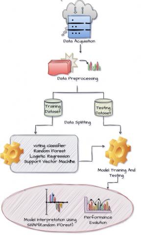
The work flow of this proposed work goes as shown in Figure 1.
Figure 1. Methodology
Performance evaluation
Performance evaluators in ML are metrics or measures used to evaluate the accuracy and potency of a model in making predictions on new data. They help to compare different models and identify areas for improvement [18].
Confusion matrix:
A 2×2 confusion matrix is a standard matrix used to assess the performance of binary classification models. It consists of four cells that represent the four possible outcomes of a binary classification problem, as shown in Figure 2.
Figure 2. Confusion matrix (for Voting Classifier)
Eqns. (1), (2), (3) and (4) are the formulae for the metrics calculation.
Accuracy: The proportion of percentage of correctly predicted labels to the total number of predictions.
Accuracy $=\frac{T P+T N}{T P+F P+T N+F N} \times 100$ (1)
Precision: The proportion of correctly predicted positives to the total predicted positives.
Precision $=\frac{T P}{(T P+F P)} \times 100$ (2)
Recall: The proportion of correctly predicted positives to the actual total positives.
Recall $=\frac{T P}{T P+F N}$ (3)
F1-score: The harmonic mean of recall and precision.
$F 1-$ Score $=2 \times \frac{\text { Precision } * \text { sensitivity }}{\text { Precision }+ \text { sensitivity }} \times 100$ (4)
SHAP
SHAP (SHapley Additive exPlanations) [19] is a model-agnostic technique for describing the predictions of ML models. It is based on the notion of Shapley values, where each feature is assigned with a value in a prediction based on how much it contributed to the outcome. In the context of Machine Learning, these values measure the impact of each feature on the model's prediction for a particular data point. They provide a detailed understanding of how the model arrived at its decision by quantifying the influence of each feature on the output. By utilizing SHAP values, it is possible to identify the most influential features in a prediction and visualize how they contribute to the final result. This can help to improve model interpretability, identify biases, and facilitate more effective decision-making in Machine Learning applications [20].
By providing feature-level explanations of model predictions, SHAP can help healthcare professionals understand how a model is making its decisions, which can lead to better trust and adoption of these models. It ensures that models are fair and transparent, which is essential for ethical use in the medical domain [21-23].
4.1 Outcomes of models
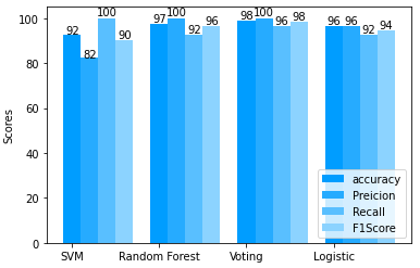
The dataset is splitted into training and testing sets into 80% and 20% respectively. According to the evaluations matrices Voting Classifier with soft voting showed an average classification accuracy of 98%, f1-score of 97.4%, precision of 95%, recall of 100%. Random Forest classifier showed an average classification accuracy of 96%, f1-score of 95%, precision of 90.4%, recall of 100%. Logistic Regression classifier showed an average classification accuracy of 94%, f1-score of 92.6%, precision of 86.3%, recall of 100%. Support Vector Machine classifier showed an average classification accuracy of 90%, f1-score of 88.3%, precision of 79.1%, recall of 100%. The values are shown in Figure 3 and Table 2.
Figure 3. Graphical representations of models’ performance
Table 2. Performance evaluation
|
|
Accuracy |
Precision |
Recall |
F1 Score |
|
SVM |
0.925 |
0.823 |
1.0 |
0.903 |
|
RF |
0.975 |
1.0 |
0.924 |
0.963 |
|
Voting Classifier |
0.985 |
1.0 |
0.964 |
0.981 |
|
LR |
0.962 |
0.963 |
0.926 |
0.945 |
Feature interpretation
Here, SHAP is applied on Random Forest model using training dataset. SHAP plots [5] that are used for visualization and interpretation of output of models are plotted:
It shows top 20 features. Larger values are indicated with red shades and smaller values are indicated with blue shades.
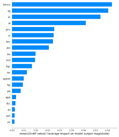
4.2 SHAP feature importance
In SHAP feature importance graph the features with large absolute Shapley values are considered as important. Since it is the global importance average of the absolute Shapley values per feature is taken across the data features are plotted in decreasing importance. The graph will be as shown in the Figure 4.
Figure 4. Shapley values per feature
The x-axis represents the average feature's contribution to the model's output across all samples in the dataset. It represents the mean absolute SHAP value. The y-axis represents the attributes.
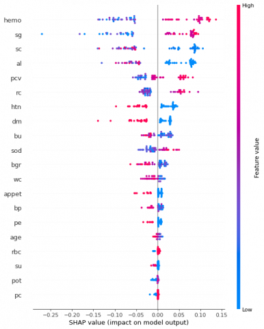
4.3 Summary plot
The summary plot combines information about feature importance and its effects. The Shapley value for each point on the plot is associated with a particular feature. Each point's y-axis position is associated to the feature, and its x-axis position is associated to its Shapley value. The graph will be as shown in the Figure 5.
Figure 5. Summary plot for Random Forest
It shows top 20 features. Larger values are indicated with red shades and smaller values are indicated with blue shades.
While the summary plot provides the basic comprehension of the relation between the value of an attribute and its influence on the outcome, the exact relationship is provided dependence plots. These plots offer a more detailed view of how the values of individual features affect the model's predictions.
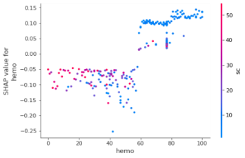
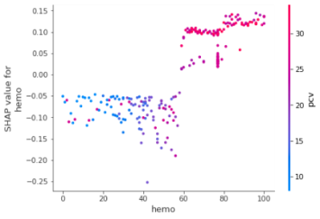
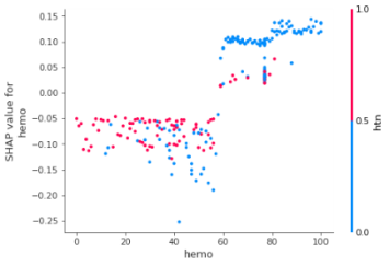
4.4 Dependence plot
It plots a point for every data instance by considering one particular feature. X-axis shows the feature value whereas y-axis shows the associated Shapely value. It is displayed like a scatter plot. The graph will be as shown in the Figure 6.
|
(a) |
(b) |
|
(c) |
(d) |
|
(e) |
(f) |
Figure 6. Dependence plots for attribute hemoglobin and other top 6 attributes (a) specific gravity, (b) serum creatinine (c) albumin (d) albumin (e) packed cell volume (f) red blood cell count
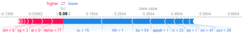
4.5 Force plot
Figure 7. Force plot
A force plot displays the SHAP values for one instance.
It shows each attribute’s contribution to the prediction for a single instance. It shows the direction and magnitude for feature's impact on the output for that instance. It displays a bar for each feature. The bar length indicates the magnitude of the attribute's effect on the predicted output. Color represents whether the feature value is high or low relative to the average value for that feature in the dataset. The force plot can help identify which features are driving the model's predictions for a given instance, and at what extent the feature contributes to the overall output. The graph will be as shown in the Figure 7.
Figure 7 shows the deviation from base value. Selected instance had the low prediction risk. Risk-increasing factors like hemo, al balance out the risk-decreasing factors such as sc,htn,bu.
This paper has explored a Machine Learning approach for predicting Chronic Kidney Disease (CKD) using a dataset from the UCI Machine Learning Repository. Data preprocessing steps, including data cleaning, feature selection, and feature scaling are performed. The models Logistic Regression (LR), Random Forest (RF), Voting Classifier and Support Vector Machine (SVM) are trained and evaluated using various metrics to estimate their performance. SHAP values cannot be used for causal inference. This is the process of finding the true causes of an event/target. SHAP values tell us how each model feature has contributed to a prediction. They do not tell us how the features contributed to the target variable.
Overall, the results demonstrate that Machine Learning can be a powerful tool for predicting CKD, and that the Voting Classifier and Random Forest performed well and Random Forest model with SHAP values can provide useful insights into the underlying patterns and relationships in the data.
This work can be extended by working on detecting the stages of CKD. Since this paper used a nominal dataset, it can be extended by taking a large set of records. A mobile or web application can also be developed which will be available for people, clinics and laboratories to test themselves with their clinical test results.
[1] Chen, G., Ding, C., Li, Y., Hu, X., Li, X., Ren, L., Ding, X., Tian, P., Xue, W. (2020). Prediction of chronic kidney disease using adaptive hybridized deep convolutional neural network on the internet of medical thing platform. IEEE Access, 8: 100497-100508. https://doi.org/10.1109/ACCESS.2020.2993546
[2] Antony, L., Azam, S., Ignatious, E., Quador, R., Beerravolu, A.R., Jonkman, M., De Boer, F. (2021). A comprehensive unsupervised framework for chronic kidney disease prediction. IEEE Access, 9: 126481-126501. https://doi.org/10.1109/ACCESS.2021.3112995
[3] Ogunleye, A., Wang, Q. (2020). XGBoost Model for Chronic Kidney Disease Diagnosis. IEEE/ACM Transactions on Computational Biology and Bioinformatics, 17(6): 2131-2139. https://doi.org/10.1109/TCBB.2019.2903401
[4] Elkholy, S.M.M., Rezk, A., Saleh, A.A.E.F. (2021). Early prediction of chronic kidney disease using deep belief network. IEEE Access, 9: 135542-135549. https://doi.org/10.1109/ACCESS.2021.3114317
[5] Emon, M.U., Imaran, A.M., Islam, R., Keya, M.S., Zannat, R., Ohidujjaman. (2021). Performance analysis of chronic kidney disease through machine learning approaches. In Proceedings of the 6th International Conference on Inventive Computation Technologies (ICICT), Coimbatore, India, pp. 713-719. https://doi.org/10.1109/ICICT50816.2021.9358534
[6] Islam, A.U., Ripon, S.H. (2019). Rule induction and prediction of chronic kidney disease using boosting classifiers, ant-miner and J48 decision tree. In Proceedings of the International Conference on Electrical, Computer and Communication Engineering (ECCE), Cox'sBazar, Bangladesh, pp. 1-6. https://doi.org/10.1109/ECACE.2019.8864520
[7] Damodara, K., Thakur, A. (2021). Adaptive neuro fuzzy inference system based prediction of chronic kidney disease. In Proceedings of the 7th International Conference on Advanced Computing and Communication Systems (ICACCS), Coimbatore, India, pp. 973-976. https://doi.org/10.1109/ICACCS51316.2021.9373848
[8] Santini, G., Moreau, N., Rubeaux, M. (2019). Kidney tumor segmentation using an ensembling multi-stage deep learning approach. A Contribution to the KiTS19 Challenge. Journal of Imaging, 5(11): 118. https://doi.org/10.3390/jimaging5110118
[9] Pushpalatha, S., Stella, A. (2021). Kidney disease diagnosis using classification algorithm. In Proceedings of the International Conference on Innovations in Smart and Modern Computing (I-SMAC), Palladam, India, pp. 1285-1288. https://doi.org/10.1109/I-SMAC51045.2021.9472260
[10] Mahbub, N.I., Hasan, M.I., Ahamad, M.M., Aktar, S., Moni, M.A. (2022). Machine learning approaches to identify significant features for the diagnosis and prognosis of chronic kidney disease. In Proceedings of the International Conference on Innovations in Science, Engineering and Technology (ICISET), Chittagong, Bangladesh, pp. 312-317. https://doi.org/10.1109/ICISET54385.2022.9712710
[11] Samet, S., Laouar, M.R., Bendid, I. (2021). Predicting and staging chronic kidney disease using optimized random forest algorithm. In Proceedings of the International Conference on Information System and Advanced Technologies (ICISAT), Tebessa, Algeria, pp. 1-6. https://doi.org/10.1109/ICISAT52747.2021.9451031
[12] Pavithra, D., Vanithamani, R. (2021). Chronic kidney disease detection from clinical data using CNN. In Proceedings of the IEEE International Conference on Distributed Computing, VLSI, Electrical Circuits and Robotics (DISCOVER), Nitte, India, pp. 1-5. https://doi.org/10.1109/DISCOVER53249.2021.9515264
[13] Vijayalakshmi, A., Sumalatha, V. (2020). Survey on diagnosis of kidney disease using machine learning algorithms. In Proceedings of the 3rd International Conference on Intelligent Sustainable Systems (ICISS), Thoothukudi, India, pp. 590-595. https://doi.org/10.1109/ICISS48214.2020.9123169
[14] Raju, N.V.G., Lakshmi, K.P., Praharshitha, K.G., Likhitha, C. (2019). Prediction of chronic kidney disease (CKD) using data science. In Proceedings of the International Conference on Intelligent Computing and Control Systems (ICICCS), Madurai, India, pp. 642-647. https://doi.org/10.1109/[ICCONS](poe://www.poe.com/_api/key_phrase?phrase=ICCONS&prompt=Tell%20me%20more%20about%20ICCONS.).2019.8941992.
[15] Sisodia, D.S., Verma, A. (2017). Prediction performance of individual and ensemble learners for chronic kidney disease. In Proceedings of the International Conference on Inventive Computing and Informatics (ICICI), Coimbatore, India, pp. 1027-1031. https://doi.org/10.1109/ICICI.2017.8360120
[16] Johari, A.A., Wahab, M.H.A., Mustapha, A. (2019). Two-class classification: comparative experiments for chronic kidney disease. In Proceedings of the 4th International Conference on Information Systems and Computer Networks (ISCON), Mathura, India, pp. 789-792. https://doi.org/10.1109/ISCON.2019.8930459
[17] Maurya, A., Wable, R., Shinde, R., John, S., Jaadhav, R., Dakshyani. (2019). Chronic kidney disease prediction and recommendation of suitable diet plan by using Machine Learning. In Proceedings of the International Conference on Nascent Technologies in Engineering (ICNTE), Navi Mumbai, India, pp. 1-5. https://doi.org/10.1109/ICNTE.2019.8849186
[18] Chen, C.J., Pai, T.W., Fujita, H., Lee, C.H., Chen, Y.T., Chen, K.S. (2014). Stage diagnosis for chronic kidney disease based on ultrasonography. In Proceedings of the 11th International Conference on Fuzzy Systems and Knowledge Discovery (FSKD), Xiamen, China, pp. 525-530. https://doi.org/10.1109/FSKD.2014.6980836
[19] Lundberg, S.M., Lee, S.I. (2017). A unified approach to interpreting model prediction. In Proceedings of the Neural Information Processing Systems (NIPS), pp. 4765-4774. https://proceedings.neurips.cc/paper/2017/file/8a20a8621978632d76c43dfd28b67767-Paper.pdf.
[20] https://www.healthdata.org/gbdttps://www.thelancet.com/journals/lancet/article/PIIS0140-6736(19)32977-0/fulltext
[21] Shilaja, K., Seetharamulu, B., Jabbar, M.A. (2018). Machine learning in healthcare: A review. In Proceedings of the 2nd International Conference on Electronics, Communication and Aerospace Technology (ICECA), pp. 910-914. https://doi.org/ 10.1109/ICECA.2018.8474918
[22] Khrisat, M., Alqadi, Z. (2023). Performance evaluation of ANN models for prediction. Acadlore Transactions on AI and Machine Learning, 2(1): 13-20. https://doi.org/10.56578/ataiml020102
[23] Ravishankar, K., Devaraj, P., Hanumathaiah, S.K.Y. (2023). Floor segmentation approach using FCM and CNN. Acadlore Transactions on AI and Machine Learning, 2(1): 33-45. https://doi.org/10.56578/ataiml020104