Pankaj Prusty*![]() | Bibhu Prasad Mohanty
| Bibhu Prasad Mohanty![]()
© 2023 IIETA. This article is published by IIETA and is licensed under the CC BY 4.0 license (http://creativecommons.org/licenses/by/4.0/).
OPEN ACCESS
We propose a novel algorithm for classification of road surfaces which can be used in intelligent vehicle for helping the driver. In a broad sense the road surfaces are classified as smooth and rough road surface. Smooth road surfaces are cement, sand and asphalt road surface where as rough road surfaces are rough asphalt and grass road surfaces. Two features are being proposed to classify smooth and rough road surfaces by analysing the intensity pattern of road surfaces and then they are classified with the help of a probabilistic classifier. After that lane detection method is used to distinguish sand road from asphalt and cement road surfaces. Then simple image processing techniques like edge and histogram analysis are used to identify remaining individual road surfaces. All works are being done in intensity plane.
ADAS, temporal depth, Mean Absolute Deviation, edge, intelligent vehicle
In today’s digital world many manual works are going to be automated with the help image processing and computer vision algorithms. The role of artificial intelligence and the environment perception of images are quite high when used in such vision based systems. Artificial Intelligence can be trained on images of road surfaces to detect variations and irregularities in the road, such as cracks, potholes, or surface texture. This can be done using techniques such as convolutional neural networks (CNNs) or other machine learning algorithms. One of the vision based application is the classification of different types of smooth and rough road surfaces which can help the driver for automated systems. The road surfaces are flat planes and hence cannot be captured by using radar and lidar sensors. However the surrounding environment around a vehicle can be captured using these sensors. Many vision based algorithms have been proposed earlier to detect lane marks, symbolic marks, potholes etc., which helps the driver in automated systems. Fan et al. [1] tried to find out a method where pothole can be detected with the help of a disparity map. They have tried to find out a computationally effective algorithm with the help of golden section search, dynamic programming, Otsu’s thresholding etc. But to get real time images in their method is quite difficult for further processing. Also different road surfaces have different issues while detecting potholes. Gupta et al. [2, 3] proposed a method for lane detection and road surface marking which is based on spatio-temporal clustering algorithm coupled with curve-fitting. They have also used Grassmann manifold algorithm for accurate detection of road surface markings. Their focus is completely on lane detection but if any road surface where lane is not there may gives rise to false detection in some cases. Guan et al. [4] discussed the development of automated algorithms which describes the extraction of different road features like road surfaces, pavement cracks, road markings etc., using the data available in mobile laser scanning point cloud. The surface extraction algorithm is capable of detecting road curbs from a group of profiles which are being sliced along the trajectory way of the vehicle. They have identified the cracks with low contrast, low SNR and poor continuity and also the road markings that which has very high retro reflectivity. When we will go for road surface detection algorithm in real time, the efficiency of this algorithm cannot be predicted because all the works are done in a specified data set. A very effective lane detection method [5] is being explained where lane can be detected by creating a background model of road surfaces and continuous up gradation of this model. This may help a driver in an automated system for lane mark identification for safety of the vehicle. The simplicity of the algorithm makes it robust and we have also taken reference of this paper in one of the module of our work. Lv et al. [6] proposed a better method which can identify the lane marks by considering confidence area detection along with field inference. They have also used a constraint regression function to consider the geometric relationship between markings of the lane and area of the lane. But because of the complexity of this algorithm, it cannot be further used as any part of other algorithms. Raj et al. [7] proposed a unique way of classifying road surfaces in two broad categories like smooth road surface and rough road surface. They have used simple image processing techniques like histogram, edge detection etc. to classify individual road surfaces, which will not work with different camera parameters or different environment. By analyzing the pattern of smooth and rough road surfaces, we have proposed two different features in temporal direction and classified the road surfaces as smooth or rough with the help of a classifier. We have considered the same sand road, asphalt and cement road as smooth road surfaces whereas grass road and rough/ rough asphalt road are treated as rough road surfaces. Hsu et al. [8, 9] proposed a method for driving area of the road need to be identified from photographs taken by a camera mounted on a vehicle. They have taken the statistical feature into consideration for this work. But the procedure of taking images for analysis are quite practical and we have also adopted the same method. Kucukmanisa and Urhan [10] explained a method which helps in advanced driver assistance system (ADAS) by identifying the vanished lane marks from road surfaces. They have considered a particular region around a pixel where center of gravity is computed using RGB histogram of the image. A method [11] is being proposed with the help of CNN to distinguish between paved and unpaved road surfaces. Also, they have identified the damage condition of road surfaces. A very interesting and fundamental work was done by Dai et al. [12] wherein the street view path images are downloaded, the vanishing image points are identified and then the road surfaces are identified. The brick and asphalt road surface images are considered as training data set. These vanished lane marks, image points, paved or unpaved road surfaces can create major issues in road surface detection algorithm in real time. For any real time approach these points need to be addressed as issues for future processing.
In our algorithm to classify rough and smooth road surfaces, we have exploited the temporal characteristics of road surfaces. Based on these characteristics, we have proposed two unique features temporal depth and Mean Absolute Deviation. These two features are sufficient enough to classify smooth and rough road surfaces. After that individual road surfaces are identified with the help of basic features like edge [13-15], histogram [16-18] etc.
The rest of the paper is organized as follows. Section 2 contains the details of our propose algorithm. Section 3 contains the result analysis of our algorithm followed by in Section 4 conclusion and references.
To distinguish between all the different categories of road surfaces, it has been categorized in two broad divisions: smooth road surfaces and rough road surfaces. Smooth road surface includes sand, asphalt and cement road where as rough road includes grass and rough road (which includes the rough asphalt road also). We will analyse separately both smooth and rough road surfaces to classify them.
2.1 Smooth and rough road surface classification
Figure 1. Intensity variation of different smooth and rough road surfaces
At first before going for any classification, it is assumed that at first our camera has captured a few frames from the road surfaces for analysis. It has been observed that the fluctuation of intensity over mean is symmetric for smooth surfaces and asymmetric for rough surfaces when considered in temporal direction. Figure 1 illustrates the variation of intensity of different smooth and rough road surfaces in temporal direction.
Observing the variation of intensity of the road surfaces over mean, we have proposed two features: temporal depth and Mean Absolute Deviation.
2.1.1 Temporal depth
In this property we have tried to find out the difference between maximum and minimum values of pixel intensity in a particular location which is defined in Eq. (1).
Temporal Depth $(\mathrm{p}, \mathrm{q})=\mathrm{abs}(\max (\mathrm{t})-\min (\mathrm{t}))$ (1)
where, t=f(p, q, i) $\forall i$ f represents the stalk of frames initially captured by the camera. The value of ‘i’ which represents the total number of frames used for decision making and it is empirically decided.
2.1.2 Mean Absolute Deviation (MAD)
In this property we have calculated the mean and then the sum of absolute deviation of intensity values from this mean is called as Mean Absolute Deviation which is represented in Eq. (2).
$\operatorname{MAD}(\mathrm{p}, \mathrm{q})=\sum_{s=0}^i|t(s)-\operatorname{mean}(t)|$ (2)
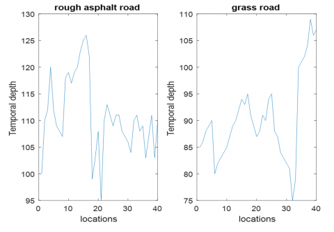
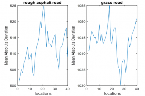
where, ‘i’ is same as calculated in Eq. (1). MAD stands for Mean Absolute Deviation. Figures 2 and 3 clearly show that the feature temporal depth and Mean Absolute Deviation are significantly able to classify the smooth road surfaces from rough road surfaces.
(a) Temporal depth variation of different smooth road surfaces
(b) Temporal depth variation of different rough road surfaces
Figure 2. Temporal depth variation of different smooth and rough road surfaces
(a) Mean Absolute Deviation variation of different smooth road surfaces
(b) Mean Absolute Deviation variation of different rough road surfaces
Figure 3. Mean Absolute Deviation variation of different smooth and rough road surfaces
2.1.3 Naive bayes classifier
The above two features are sufficient to classify smooth and rough road surfaces. To classify we have taken the help of naïve Bayes classifier where the most probable decision rule that is MAP decision rule is being used for classification. By taking a prior probability of a given hypothesis Bayes Theorem [19-21] gives a method to find out the probability of the hypothesis. To classify, the corresponding classifier function is defined as,
$\begin{aligned} \text { Classify }(\mathrm{n} 1, \mathrm{n} 2, \ldots \mathrm{nn})=\operatorname{argmax} P(X \\ =x) \prod_{i=1}^N P(L i=n i \mid X=x)\end{aligned}$ (3)
where, X represents the conditional class variable with few classes and Li represents the feature variable.
2.2 Distinguishing asphalt, cement road and sand road
It is quite obvious that smooth asphalt and smooth cement road must contain lane marks whereas sand road does not contain any lane mark. If lane mark is being identified in any of the smooth road then that can be treated as cement or asphalt road surfaces and the road surfaces with no lane mark is treated as sand road surfaces. We tried to detect the lane marks as described in the study [5]. Initially a model is being created with the help of non-lane areas. Then individual pixel is being tested with two empirically calculated threshold values to classify a pixel as lane or non-lane. If around 20% of pixels are being classified as lane pixel from any frame we consider it as asphalt or cement road and if no lane mark is being detected we classify it as sand road. Once sand road is being identified, our aim is to distinguish between asphalt and cement road. As both of them contain lane marks, hence it is not possible to distinguish them by considering lane marks only. To distinguish between them be have taken the method as proposed by Raj et al. [6]. According to them both asphalt and cement road have gray color structure which differentiates them from others. But to distinguish between them Canny edge detection method works fine. Figure 4 shows the distinguition between numbers of edges between cement and asphalt roads.
Figure 4. No of edges of cement and asphalt road surfaces
2.3 Distinguishing grass road, rough or rough asphalt road
As described by Raj et al. [6] histogram plays a vital role in classifying grass road and rough road surfaces. It is obvious that the intensity values of grass are widely distributed in a certain range in comparison to rough road. If range of intensity between LTH and UTH, where 3/4th of total number of pixels reside is classified as grass road and other roads are rough or rough asphalt road as described in Eq. 4. ITOT represents the total number of pixels in a frame.
$L_{T H}<\frac{3}{4} I_{T O T}<U_{T H}$ (4)
Experimentally it has been observed that the range of values of two threshold lies in the range of 100-200. Figure 5 shows the validity of Eq. (4) with threshold values in between 100 to 200.
Figure 5. The intensity histogram of different road surface
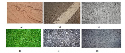
Our algorithm has been evaluated by a data set created by us. The data set consists of image frames which has been extracted from videos taken using a mobile phone camera. Also while taking the videos, it has been assumed that the camera is mounted on the hood of the moving vehicle. The implementation of our proposed algorithm has been done in MATLAB 2016 in windows 10 operating system. The algorithm was run in a laptop system with Intel Core (TM) i3-3110M CPU with clock speed of 2.4 GHZ and with a RAM of 4GB and a 64 bit operating system. Figure 6 shows one frame each from all the different videos that we have used as rough and smooth road surfaces. Though our algorithm works on videos but individual frames are being considered for prediction of the road surfaces. Six different categories of videos are used for simulation which are sand, asphalt, cement, grass, rough and rough asphalt road surfaces. These videos consist of 260,431,556, 422, 544,621 frames respectively. Our frame size is 320 x 420 for processing of data sets. To predict the Rth frame as smooth or rough road surface we need to analyse R-(N/2-1) to R+(N/2+1) frames. N need to be calculated empirically as shown in Table 1. As per our observation which is shown in Table 1, temporal window size 10 is sufficient to consider. If we choose a temporal window size more than 10, there is no significant change in accuracy of the algorithm. So to maintain better processing speed we have chosen the value of N as 10. The measurement of accuracy is being described in the later part of this section. Once temporal window size is fixed, then our job is to differentiate smooth and rough road surfaces for which we have taken the help of naïve Bayes classifier. Two features have been proposed: temporal depth and Mean Absolute Deviation, which are described in previous section. At first it is required to create a data set for smooth and rough road surfaces which can be fed to the classifier. In the beginning N consecutive frames from different smooth and rough road surfaces are taken. Randomly 100 locations are taken from each video. For each location from the stack of N frames the above said two features are calculated. Now we have 300 data sets for each smooth and rough road surfaces. All these 600 different data set values are being used to train the classifier. After the classifier is being trained, the (N+1)th frame is being taken for testing purpose. At first one pixel location is considered for observation. But it has been observed that sometimes it becomes very difficult to predict the exact smooth or rough road surface with the help of a single location. So to predict a frame as smooth or rough we need to choose R random pixels and out of these R if P no of pixels are predicted as rough, then entire frame is predicted as rough else smooth. The value of R and P are decided empirically. In our case we have chosen the value of R to be 20 and P to be 50% of R, i.e., 20. Table 2 says the no of correctly classified frames as smooth and rough road surfaces. The accuracy can be calculated using Eq. (5).
$\begin{aligned} & \text { Accuracy } \\ & =\frac{\text { No of correctly classified frames }}{\text { Total no of frames used for testing }} \times 100\end{aligned}$ (5)
Table 1. Accuracy variation with different temporal window size
|
|
Smooth Road Surfaces Accuracy (%) |
Rough Road Surfaces Accuracy (%) |
|||
|
Temporal Window Size |
Sand Road |
Asphalt Road |
Cement Road |
Grass Road |
Rough Asphalt Road |
|
4 |
4 |
12 |
16 |
13 |
25 |
|
6 |
38 |
27 |
30 |
25 |
27 |
|
8 |
72 |
83 |
81 |
65 |
78 |
|
10 |
88 |
95 |
92 |
85 |
89 |
|
12 |
88 |
95 |
92 |
85 |
89 |
|
14 |
89 |
93 |
91 |
84 |
85 |
|
16 |
88 |
94 |
90 |
84 |
85 |
|
18 |
87 |
91 |
90 |
81 |
81 |
Table 2. No of correctly classified frames as rough and smooth road surfaces
|
|
No of frames tested |
Classified as smooth |
Classified as rough |
Accuracy (%) |
|
|
Smooth |
Sand |
100 |
82 |
18 |
82 |
|
Asphalt |
100 |
85 |
15 |
85 |
|
|
Cement |
100 |
92 |
08 |
92 |
|
|
Rough |
Grass |
100 |
14 |
86 |
86 |
|
Rough Asphalt |
100 |
09 |
91 |
91 |
|
Table 3. Comparison of vision based algorithm and proposed algorithm
|
|
No of frames tested |
Correct classified frames using probabilistic method |
Accuracy of proposed method (%) |
Accuracy of vision based method (%) |
|
|
Smooth |
Sand |
200 |
186 |
93 |
91 |
|
Asphalt |
200 |
182 |
91 |
85 |
|
|
Cement |
200 |
175 |
87.5 |
85 |
|
|
Rough |
Grass |
200 |
190 |
95 |
86 |
|
Rough Asphalt |
200 |
188 |
94 |
86 |
|
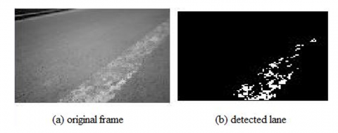
After classification of smooth and rough road surfaces, it is our job to predict the exact road surfaces, i.e., if it is classified as smooth, then it is sand, asphalt or cement and if it is classified as rough then whether it is grass or rough/ rough asphalt. From the smooth classified road surfaces, lane mark is tried to be identified as described in above section. Figure 7 shows a sample frame from road surfaces where lane is being detected using [5]. If lane is detected from a frame, then it can be a cement or asphalt road and if no lane is there then it can be treated as a sand road. Figure 7 represents the detected lane mark from an asphalt road surface. Because sand road never contains lane mark, so the category of smooth road surface with no lane mark is classified as sand road surface and the other road surfaces may be either asphalt or cement road assuming that lane is present in both these road surfaces. If a road surface is not classified as sand road, then we need to test it to classify either as asphalt or cement road. As explained in previous section Raj et al. [7] found out that edge is an important parameter to classify asphalt and cement road. Depending upon this edge we have classified asphalt and cement road, where canny edge detection method is used to detect the edges. Any other edge detection method can also be used for this purpose. A threshold value is decided initially which can distinguish edges from two different frames. Any value between 14500 to 15000 is fine to be the threshold value. Then we have to classify rough road surfaces. Two different rough road surfaces are considered, rough or rough asphalt and grass road surfaces. Only histogram analysis is sufficient in classifying these two road surfaces. As explained in Eq. (4) a suitably chosen threshold is sufficient to distinguish grass road from rough road surfaces. Finally our probabilistic method result is being compared with vision based road surface method [7]. Table 3 shows a brief comparison between these two methods, which proves that the probabilistic method gives quiet better result in predicting road surfaces.
Figure 6. Different types of road surfaces (a) sand (b) asphalt (c) cement (d) grass (e) rough (f) rough asphalt
Figure 7. Original frame and detected lane mark from an asphalt road surfaces
We have proposed a novel probabilistic road surface classification method which uses a probabilistic classifier and it classify smooth and rough road surfaces with the help of two features which are considered by analysing the intensity variation temporally. The two features are unique because these are being considered by varying the intensity temporally. Any types of noise or some other atmospheric turbulances which can degrade the quality of the image will not have any impact on the accuracy of the algorithm because of these temporal characterstics. The method used for lane detection is is less time consuming in nature which makes the algorithm roubust. Simple image processing techniques like edge and histogram towards the last section in this big classification problem makes it more user friendly. The accuracy of the algorihm shows how computationally efficient the algorithm is. This algorithm works only in intensity plane without taking the colour components into consideration and this make the algorithm more effective. Initial knowledge about the road surfaces needs to be known to train the classifier and the model need to be updated at regular intervals. This model will help a driver in autonomous driving and ADAS in intelligent vehicles. We have evaluated our system on a data set created by us and compared it with one existing algorithm. Though much more algorithms on complete classification of all road surfaces are not developed up to a significant extent, this algorithm will work as a beginning mile stone for such experiment.
[1] Fan, R., Ozgunalp, U., Hosking, B., Liu, M., Pitas, I. (2019). Pothole detection based on disparity transformation and road surface modeling. IEEE Transactions on Image Processing, 29: 897-908. https://doi.org/10.1109/TIP.2019.2933750
[2] Gupta, A., Choudhary, A. (2018). A framework for camera-based real-time lane and road surface marking detection and recognition. IEEE Transactions on Intelligent Vehicles, 3(4): 476-485. https://doi.org/10.1109/TIV.2018.2873902
[3] Zakaria, N.J., Shapiai, M.I., Ghani, R.A., Yasin, M.N. M., Ibrahim, M.Z., Wahid, N. (2023). Lane detection in autonomous vehicles: A systematic review. IEEE Access. 11: 3729-3765. https://doi.org/10.1109/ACCESS.2023.3234442
[4] Guan, H., Li, J., Yu, Y., Chapman, M., Wang, C. (2014). Automated road information extraction from mobile laser scanning data. IEEE Transactions on Intelligent Transportation Systems, 16(1): 194-205. https://doi.org/10.1109/TITS.2014.2328589
[5] Prusty, P., Mohanty, B. (2020). A framework for real-time lane detection using spatial modelling of road surfaces. In Advances in Intelligent Computing and Communication: Proceedings of ICAC 2019, Springer Singapore, pp. 135-140. https://doi.org/10.1007/978-981-15-2774-6_17
[6] Lv, H., Liu, C., Zhao, X., Xu, C., Cui, Z., Yang, J. (2020). Lane marking regression from confidence area detection to field inference. IEEE Transactions on Intelligent Vehicles, 6(1): 47-56. https://doi.org/10.1109/TIV.2020.3009366
[7] Raj, A., Krishna, D., Priya, R.H., Shantanu, K., Devi, S.N. (2012). Vision based road surface detection for automotive systems. In 2012 International Conference on Applied Electronics, Pilsen, Czech Republic, pp. 223-228.
[8] Hsu, C.M., Lian, F.L., Lin, Y.C., Huang, C.M., Chang, Y.S. (2012). Road detection based on region similarity analysis. International Conference on Automatic Control and Artificial Intelligence, 1775-1778.
[9] Badrloo, S., Varshosaz, M., Pirasteh, S., Li, J. (2022). Image-based obstacle detection methods for the safe navigation of unmanned vehicles: A review. Remote Sensing, 14(15): 3824. https://doi.org/10.3390/rs14153824
[10] Kucukmanisa, A., Urhan, O. (2016). Histogram distance based road surface detection on a single image. International Journal of Transportation Systems, 1: 84-91.
[11] Rateke, T., Von Wangenheim, A. (2021). Road surface detection and differentiation considering surface damages. Autonomous Robots, 45: 299-312. https://doi.org/10.1007/s10514-020-09964-3
[12] Dai, J.M., Liu, T.A.J., Lin, H.Y. (2017). Road surface detection and recognition for route recommendation. In 2017 IEEE Intelligent Vehicles Symposium (IV) Los Angeles, CA, USA, pp. 121-126. https://doi.org/10.1109/IVS.2017.7995708
[13] Ding, L., Goshtasby, A. (2001). On the Canny edge detector. Pattern recognition, 34(3): 721-725. https://doi.org/10.1016/S0031-3203(00)00023-6
[14] Reddy, R.P.K., Nagaraju, C., Reddy, I.R. (2016). Canny scale edge detection. International Journal Eng Trends Technol (IJETT). https://doi.org/10.14445/22315381/IJETT-ICGTETM N, 3.
[15] Nain, G., Pattanaik, K.K., Sharma, G.K. (2022). Towards edge computing in intelligent manufacturing: Past, present and future. Journal of Manufacturing Systems, 62: 588-611. https://doi.org/10.1016/j.jmsy.2022.01.010
[16] Nuzzo, R.L. (2019). Histograms: A useful data analysis visualization. PM&R, 11(3): 309-312. https://doi.org/10.1002/pmrj.12145
[17] Boels, L., Bakker, A., Van Dooren, W., Drijvers, P. (2019). Conceptual difficulties when interpreting histograms: A review. Educational Research Review, 28: 100291. https://doi.org/10.1016/j.edurev.2019.100291
[18] Kumar, D.P., Muralidharan, V., Ravikumar, S. (2022). Histogram as features for fault detection of multi point cutting tool–A data driven approach. Applied Acoustics, 186: 108456. https://doi.org/10.1016/j.apacoust.2021.108456
[19] Mitchel, T. (1997). Machine Learning. McGraw-Hill Education (ISE Editions).
[20] Wibawa, A.P., Kurniawan, A.C., Murti, D.M.P., Adiperkasa, R.P., Putra, S.M., Kurniawan, S.A., Nugraha, Y.R. (2019). Naïve Bayes classifier for journal quartile classification. International Journal of Recent Contributions from Engineering Science & IT (IJES), 7(2): 91-99. https://doi.org/10.3991/ijes.v7i2.10659
[21] Rish, I. (2001). An empirical study of the naive Bayes classifier. In IJCAI 2001 Workshop on Empirical Methods in Artificial Intelligence, 3(22): 41-46. https://doi.org/10.1002/9781118721957.ch4