Sunardi![]() | Anton Yudhana
| Anton Yudhana![]() | Setiawan Ardi Wijaya*
| Setiawan Ardi Wijaya*![]()
© 2023 IIETA. This article is published by IIETA and is licensed under the CC BY 4.0 license (http://creativecommons.org/licenses/by/4.0/).
OPEN ACCESS
Locating the facial region is the aim of face detection in digital images. Face detection issues frequently arise because of digital image noise levels. This study uses median and means filtering techniques to reduce noise in digital photographs. A confusion matrix is used to quantify the median and means filtering methods' accuracy, while the parameters Mean Square Error (MSE) and Peak Noise to Signal Ratio (PNSR) are used to assess these approaches' performance. For this experiment, Viola-Jones was chosen as the face detection method since it is one of the face detection methods with the best accuracy and computational power. According to the outcomes of comparing the median and mean filtering techniques using MSE and PNSR on 50 image samples, the median filtering approach produced the lowest average MSE results, with a value of 19.43, and the median filtering procedure yielded a 13.74 value for the highest PNSR score. The fastest average time was obtained from the mean filtering method with a time of 3.18 seconds. As for the accuracy based on the confusion matrix, these two methods get a good accuracy of 90%. These findings indicate that the Median Filtering approach is superior to the Mean Filtering method in terms of error.
mean filtering, median filtering, MSE, PNSR, confusion matrix
The human face recognition system is very important in this era of very fast technological development [1, 2]. The algorithm must first recognize the face before human face recognition [3, 4]. However, issues frequently arise when it is determined that the image to be processed has a lot of noise. By using the Median and Mean Filtering methods and evaluating their viability for usage in the situation of face detection in digital photographs, this study resolves the issue at hand. Research using the mean filtering method had previously been conducted with a total of 30 test samples [5] and research using the median filtering method had previously been conducted with a total of 10 test samples [6]; however, the two studies were conducted independently and used different numbers of samples. Because of this, the researchers used 30 sample photos to assess the two approaches' viability and determine which one worked best. Because the median value of all previous values is used when replacing pixels, the median filtering approach was chosen because it effectively reduces noise in the image and produces a more focused image [7-9].
Since the Mean Filtering method effectively reduces picture noise and sharpens images by replacing pixel values with the average of all previous values, it was chosen [9-11]. Several criteria are employed in a confusion matrix to test the accuracy of this procedure, namely True Positive (TP), True Negative (TN), False Positive (FP), and False Negative (FN) making it easier during the calculation process [12-14]. Peak Noise to Signal Ratio (PNSR) and Mean Square Error (MSE) are used to gauge the effectiveness of this technique. The better the results, which are inversely correlated with MSE and PNSR values, the smaller the MSE value and higher the PNSR value respectively [15, 16]. MSE and PNSR were also chosen since they are simple to obtain and frequently utilized in research [17-21].
The Red Green Blue (RGB) image is input into the processing system as the first stage in the face detection process, after which the RGB image is transformed into a grayscale image [22-24]. The grayscale image is then subjected to filtering with the goal of lowering noise and improving the image so that it is simpler to process.
Viola-Jones is the technique used to find faces. This technique was chosen since it is an accurate face identification process with strong computing capabilities [3, 25]. The Viola-Jones method selects the feature values for the Cascade Classifier using Integral Image and AdaBoost after using the Haar-like feature as a descriptor. Using this classifier, we can recognize faces in digital pictures [26, 27].
The Joint Photographic Experts Group (JPEG) format, which uses a lossy compression method to degrade the quality of the image, was utilized to create the image for this study [28-30]. A camera that captures photos that are similar to the object's condition at the time of capture can record the reflection of an object as an image. The image was captured using the 13-megapixel and 5-megapixel Samsung A11 smartphone camera. The images used as samples in this study are clear landscapes, 10 sample photos with one face, 10 sample photos with two faces, 10 sample photos with three faces, 10 sample photos with four faces and 10 sample photos with 5 or more faces.
An Asus laptop with a core i3 CPU and 8 GB of memory was used for this study, along with the MATLAB a13 software and the Windows 10 pro operating system. Because MATLAB is accompanied with excellent mathematical software, graphics, and programming abilities, it is widely used. The application includes built-in features to carry out a variety of tasks [31-33].
There are four sections to this essay. The background of this study and a few relevant earlier investigations are presented in Section 1. Flowcharts and an explanation of the median and mean filtering techniques used for face detection in digital photographs are provided in Section 2. The results of tests using the mean filtering method are shown in Section 3. The use of median and mean filtering methods for face detection in digital photographs is then discussed in Section 4, with conclusions drawn about which approach is the most effective.
2.1 Object of research
A digital snapshot of a human face serves as the subject of the investigation. Research efforts aim to improve methods for identifying face objects in photographs. The images used as samples in this study are clear landscapes, 10 sample photos with one face, 10 sample photos with two faces, 10 sample photos with three faces, 10 sample photos with four faces and 10 sample photos with 5 or more faces. Table 1 provides examples of the photo samples that were used.
Table 1. Examples of sample photos used
|
No |
Sample |
Description |
|
1 |
Camera: front camera Samsung A11 with 5 megapixels resolution Date: 15 November 2021, 8:04 PM File type: JPG 1,10 MB Size: 3264x1836 px |
|
|
2 |
Camera: front camera Samsung A11 with 5 megapixels resolution Date: 16 January 2022, 4:26 PM File type: JPG 2,30 MB Size: 3264x1836 px |
|
|
3 |
Camera: front camera Samsung A11 with 5 megapixels resolution Date: 10 September 2020, 1:29 PM File type: JPG 1,27 MB Size: 3264x1836 px |
|
|
4 |
Camera: Samsung A11 with 13 megapixels resolution Date: 09 January 2023, 2:59 PM File type: JPG 2,27 MB Size: 4128x2322 px |
|
|
5 |
Camera: Samsung A11 with 13 megapixels resolution Date: 31 December 2022, 3:13 PM File type: JPG 3,27 MB Size: 4128x2322 px |
Examples of samples meeting five requirements are shown in Table 1 in accordance with the earlier description. In this study, 50 face pictures served as the sample.
2.2 Pre-processing
Pre-processing is a procedure used to improve the classification's precision and accuracy.
2.3 Filtering
Filtering is a process of improving the image to reduce the existing noise. Filtering used in this research are:
2.3.1 Median filtering
This method sorts the pixel values to make it work from the smallest to the largest value based on eight neighbors as shown in Table 2, after which the middle value is taken [7-9].
Table 2. An example of eight adjacent pixels
|
P1 |
P2 |
P3 |
|
P8 |
f(y,x) |
P4 |
|
P7 |
P6 |
P5 |
Mathematically, the filter can be Eq. (1) as follows:
Median(x, y) = P1, P2, P3, P4, P5, P6, P7, P8 (1)
After being sorted as in Eq. (1), the middle value is taken and the value in f(x, y) is replaced with that value.
2.3.2 Mean filtering
This technique replaces the pixel values with an average of all the current values [9-11]. Table 2 provides a sample of 3x3 pixels and the equation to calculate them (2):
$\operatorname{Mean}(y, x)=\frac{1}{9} \cdot(P 1, P 2, P 3, P 4, P 5, P 6, P 7, P 8)$ (2)
So the initial value of f(y, x) is changed to the value that gets Mean(y, x).
2.4 Viola-Jones
In digital photographs, face characteristics are found using the Viola-Jones approach. There are four essential components to this approach, namely:
2.4.1 Haar-like feature
Alfred Haar, a Hungarian mathematician, gave this characteristic its name in the 19th century. By showing a square with oppositely colored sides, occasionally having a lighter side on one side than the other, such as the brow's outer edge, one might identify traits that resemble those of Haar [26, 27]. The center could be more reflective than the surrounding squares, giving the impression of a nose. The Haar-like feature's dark and light sides are depicted in Figure 1.
To aid the engine in understanding what a picture is, Figure 1 depicts the dark and light sides. Each characteristic will yield a single value, with the dark side being worth -1 and the light side being worth +1. For face detection, it is also essential to consider the horizontal and vertical parameters that describe the geometry of the machine's nose and eyebrows, respectively [26, 27].
Figure 1. Haar-like feature
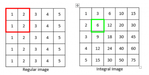
2.4.2 Integral image
Because there will be more pixels in huge features in this part, the feature values are calculated carefully. To swiftly complete complex computations and demonstrate that the characteristics of a number of features meet the requirements, an integral picture is utilized [26, 27]. An example of computing the integral image is provided in Figure 2.
Figure 2. Integral image example
There are two images in Figure 2, a standard image and an integral image. By summing the values of the regular picture according to the red line in Figure 2 one can obtain the integral image value represented by the green line.
2.4.3 AdaBoost
In order to improve accuracy, this method can actually identify the FP and TN in the data from the supplied image [26, 27].
Figure 3. Feature example
$F(x)=a_1 f_1(x)+a_2 f_2(x)+\cdots+a_n f_n(x)$ (3)
Figure 3 is an example of the features that affect the success rate. The features are f1 , f2 , and fn , and the weights are a1 , a2 , and an , each feature is referred to as a weak classifier, whereas the strong classifier is the equation. F(x) to create a powerful classifier, two or three weak classifiers must be combined. Assemblies are what happen when something is added repeatedly, and this is how adaptive boosting works [26, 27].
2.4.4 Cascaded classifier
This classifier is a shortcut to improve the model's speed and accuracy. It begins by taking a sub-window, after which it selects the most crucial or ideal qualities, making sure that they are present in the sub-image window. The sub-window won't be processed if there isn't one. If so, the sub-window will be rejected without the feature being used, and the number of features it has will continue. Cascading is utilized to speed up the machine's processing because this procedure takes a long time because it must be done for each feature [26, 27].
2.5 Result evaluation
Utilize a confusion matrix to evaluate the reliability of the mean filtering technique. This method makes the computation procedure simpler by measuring it using multiple criteria, including TP, TN, FP, and FN [12, 14]. Here is Eq. (4) to calculate accuracy:
$\operatorname{accuracy}=\frac{T P+T N}{T P+T N+F P+F N}$ (4)
PNSR and MSE are used to gauge the effectiveness of this technique. The better the results, which are inversely correlated with MSE and PNSR values, greater the PNSR value and lower the MSE value, respectively [15, 16]. Here is Eq. (5) for MSE:
$M S E=\frac{\sum_{a=0}^{x-1} \cdot \sum_{b=0}^{y-1} \cdot(M(a, b)-N(a, b))}{x * y}$ (5)
N(a, b) is the reference image, and M(a, b) is the value of the filtered image. The highest power signal to greatest power noise ratio is known as the PNSR [16]. The Eq. (6) for PNSR is as follows.
$P S N R=10 \log _{10} \frac{M a x_i^2}{M S E}$ (6)
$\operatorname{Max}_i$ is the highest pixel value in an image. The image utilized in this study has been transformed to a grayscale image, with an 8-bit bit depth and an intensity range of 0 to 255. White is represented by a number of 255 and black by a value of 0.
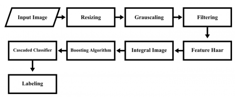
2.6 Proposed method
The approach suggested in this study uses mean filtering to find faces in digital pictures. Figure 4 shows the flowchart for this study methodology.
Figure 4. Research flow
1) Put images into MATLAB, the program used to process images.
2) In order to expedite processing, the initial photo is resized during the resizing stage.
3) Use the grayscale procedure to transform RGB-format photographs into grayscale. Utilize the following formula to turn the RGB image to grayscale:
Iy = 0.333Fr + 0.5Fg + 0.1666Fb (7)
While Iy is the intensity of gray, which is similar to an RGB level image the intensity of Red is Fr, the intensity of Green is Fg, and the intensity of Blue is Fb.
4) To reduce the noise in the image, enhance it using median or mean filtering techniques.
5) It is easy to categorize photographs based on feature values. There are a number of benefits to using features rather than pixels directly. If the function allows for the encoding of ad-hoc domain knowledge, which is difficult to recognize with little training data, that would be a very tenable explanation.
6) The integral image approach reduces the computation of the original value of each Haar-like feature at each picture position. The phrase "overall integral" refers to the weighted pixel values that will be added to the source image.
7) Weighting the representations of weak classifiers allows the boosting solution technique to merge numerous weak classifiers into strong classifiers.
8) Weights the weak classifier and combines a number of weak classifiers to create a stronger classifier. The classifier's filter order is considered weak in this context since it only accepts a limited number of accurate responses. Each step of filtering enhances the previously filtered image. If one of these filters fails, the region in the image is marked as "non-face." But this calculation method requires a lot of memory consumption, and the calculation error is large.
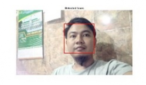
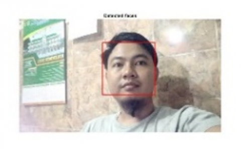
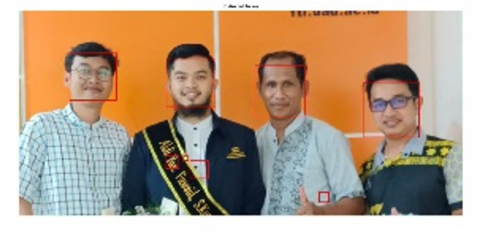
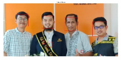
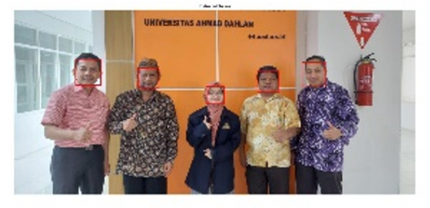
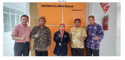
9) The face is then marked with a red line after the image has been converted into a matrix value using a method to locate the area.
50 images were utilized in this investigation, including 10 sample photos with one face, 10 sample photos with two faces, 10 sample photos with three faces, 10 sample photos with four faces and 10 sample photos with 5 or more faces.
The image was captured using the 13-megapixel main camera and 5-megapixel front camera on the Samsung A11 smartphone. The Median and Mean Filtering techniques were examined at this point. The MATLAB software with hardware support for an Intel(R) Core(TM) i3-5005U CPU running at 2.00GHz and 8 GB of RAM was used for the tests.
The following is an example of the results obtained based on the three criteria used, an example of the results is presented in Table 3 below.
Table 3. An example of the results obtained
|
No |
Samples |
Method |
Result |
|
1 |
Median |
TP MSE: 0.95 PNSR: 24.28 Speed: 3.01s |
|
|
Mean |
TP MSE: 14.92 PNSR: 12.33 Speed: 3.61s |
||
|
2 |
Median |
TN MSE: 57.44 PNSR: 6.47 Speed: 3.60s |
|
|
Mean |
TN MSE: 90.53 PNSR: 4.50 Speed: 3.62s |
||
|
3 |
Median |
TP MSE: 1.15 PNSR: 23.46 Speed: 4.64s |
|
|
Mean |
TP MSE: 11.63 PNSR: 13.41 Speed: 3.55s |
||
|
4 |
Median |
TN MSE: 0.29 PNSR: 30.96 Speed: 1.92s |
|
|
Mean |
TN MSE: 7.52 PNSR: 15.30 Speed: 1.87s |
||
|
5 |
Median |
TP MSE: 1.15 PNSR: 20.26 Speed: 2.00s |
|
|
Mean |
TP MSE: 23.94 PNSR: 10.27 Speed: 2.03s |
Table 3 displays the outcomes of processing three sample criteria from Table 1 using the median and mean filtering procedures. Table 4 below shows the full findings for the 50 samples.
Table 4. Results MSE and PNSR
|
No |
Method |
Description |
MSE |
PNSR |
Speed (s) |
|
1 |
Median |
TP |
0.95 |
24.28 |
3.01 |
|
Mean |
TP |
14.92 |
12.33 |
3.61 |
|
|
2 |
Median |
TP |
7.63 |
15.24 |
3.91 |
|
Mean |
TP |
19.59 |
11.15 |
4.90 |
|
|
3 |
Median |
TN |
4.23 |
17.80 |
3.93 |
|
Mean |
TN |
11.79 |
13.35 |
4.88 |
|
|
4 |
Median |
TN |
9.90 |
14.11 |
3.82 |
|
Mean |
TN |
20.00 |
11.05 |
4.66 |
|
|
5 |
Median |
TP |
4.92 |
17.15 |
3.55 |
|
Mean |
TN |
13.13 |
12.88 |
4.36 |
|
|
6 |
Median |
TP |
16.31 |
11.94 |
3.87 |
|
Mean |
TP |
33.05 |
8.87 |
4.78 |
|
|
7 |
Median |
TN |
19.01 |
11.28 |
3.91 |
|
Mean |
TN |
35.35 |
8.58 |
4.90 |
|
|
8 |
Median |
TN |
30.98 |
9.15 |
3.92 |
|
Mean |
TN |
51.58 |
6.94 |
4.88 |
|
|
9 |
Median |
TP |
8.60 |
14.72 |
4.12 |
|
Mean |
TP |
16.13 |
11.99 |
5.13 |
|
|
10 |
Median |
TN |
7.01 |
15.60 |
3.26 |
|
Mean |
TN |
19.56 |
11.15 |
4.04 |
|
|
11 |
Median |
TN |
57.44 |
6.47 |
3.60 |
|
Mean |
TN |
90.53 |
4.50 |
3.62 |
|
|
12 |
Median |
TP |
50.75 |
7.01 |
4.54 |
|
Mean |
TP |
72.96 |
5.43 |
4.54 |
|
|
13 |
Median |
TP |
0.87 |
24.65 |
3.85 |
|
Mean |
TN |
9.33 |
14.37 |
3.72 |
|
|
14 |
Median |
TN |
11.96 |
13.29 |
3.47 |
|
Mean |
TN |
23.39 |
10.38 |
3.50 |
|
|
15 |
Median |
TN |
5.59 |
16.58 |
3.83 |
|
Mean |
TN |
21.31 |
10.78 |
3.85 |
|
|
16 |
Median |
TP |
15.84 |
12.07 |
3.67 |
|
Mean |
TP |
31.73 |
9.05 |
3.64 |
|
|
17 |
Median |
TP |
15.29 |
12.22 |
9.98 |
|
Mean |
TN |
27.41 |
9.69 |
3.89 |
|
|
18 |
Median |
TP |
14.08 |
12.58 |
3.67 |
|
Mean |
TP |
30.98 |
9.16 |
3.53 |
|
|
19 |
Median |
TN |
45.60 |
7.48 |
4.85 |
|
Mean |
TP |
66.66 |
5.83 |
4.78 |
|
|
20 |
Median |
TP |
0.94 |
24.33 |
3.96 |
|
Mean |
TP |
10.55 |
13.83 |
3.71 |
|
|
21 |
Median |
TN |
52.33 |
6.88 |
0.79 |
|
Mean |
TN |
124.19 |
3.12 |
0.66 |
|
|
22 |
Median |
FP |
8.26 |
14.89 |
3.41 |
|
Mean |
FP |
26.01 |
9.91 |
3.39 |
|
|
23 |
Median |
TP |
1.15 |
23.46 |
4.64 |
|
Mean |
TP |
11.63 |
13.41 |
3.55 |
|
|
24 |
Median |
TN |
61.70 |
6.16 |
4.51 |
|
Mean |
TP |
102.95 |
3.94 |
3.46 |
|
|
25 |
Median |
TP |
29.22 |
9.41 |
2.35 |
|
Mean |
TP |
48.11 |
7.24 |
1.74 |
|
|
26 |
Median |
TP |
9.49 |
14.29 |
2.19 |
|
Mean |
TP |
19.59 |
11.15 |
2.91 |
|
|
27 |
Median |
FP |
10.07 |
14.04 |
4.80 |
|
Mean |
FP |
12.47 |
13.11 |
6.66 |
|
|
28 |
Median |
TN |
50.92 |
6.99 |
5.70 |
|
Mean |
TN |
74.18 |
5.36 |
5.71 |
|
|
29 |
Median |
FP |
28.27 |
9.55 |
2.33 |
|
Mean |
FP |
44.80 |
7.55 |
1.70 |
|
|
30 |
Median |
TP |
3.57 |
18.54 |
3.20 |
|
Mean |
TP |
15.11 |
12.27 |
3.12 |
|
|
31 |
Median |
TP |
5.97 |
16.31 |
1.69 |
|
Mean |
TN |
31.88 |
9.03 |
2.68 |
|
|
32 |
Median |
TP |
8.58 |
14.73 |
1.70 |
|
Mean |
TP |
45.36 |
7.50 |
1.64 |
|
|
33 |
Median |
TN |
1.11 |
23.61 |
1.77 |
|
Mean |
TN |
14.24 |
12.53 |
1.60 |
|
|
34 |
Median |
TP |
7.45 |
15.35 |
2.57 |
|
Mean |
TP |
45.36 |
7.50 |
2.42 |
|
|
35 |
Median |
TN |
0.82 |
24.91 |
2.43 |
|
Mean |
TP |
16.21 |
11.97 |
2.38 |
|
|
36 |
Median |
TP |
1.60 |
22.02 |
2.27 |
|
Mean |
TP |
16.21 |
11.97 |
2.08 |
|
|
37 |
Median |
TN |
1.95 |
21.16 |
2.17 |
|
Mean |
TN |
22.20 |
10.60 |
2.09 |
|
|
38 |
Median |
FP |
0.74 |
25.39 |
2.07 |
|
Mean |
FP |
7.29 |
15.44 |
1.96 |
|
|
39 |
Median |
TN |
0.20 |
30.96 |
1.92 |
|
Mean |
TN |
7.52 |
15.30 |
1.87 |
|
|
40 |
Median |
TN |
2.34 |
20.38 |
2.29 |
|
Mean |
TN |
13.68 |
12.71 |
2.14 |
|
|
41 |
Median |
TN |
3.97 |
18.08 |
2.18 |
|
Mean |
TN |
23.47 |
10.36 |
2.17 |
|
|
42 |
Median |
TN |
7.91 |
15.09 |
3.97 |
|
Mean |
TN |
43.02 |
7.73 |
2.18 |
|
|
43 |
Median |
TN |
1.13 |
23.53 |
2.01 |
|
Mean |
TN |
14.09 |
12.57 |
2.01 |
|
|
44 |
Median |
TN |
0.54 |
26.73 |
1.97 |
|
Mean |
TN |
9.66 |
14.22 |
1.95 |
|
|
45 |
Median |
TN |
1.07 |
23.77 |
1.99 |
|
Mean |
TP |
15.76 |
12.09 |
1.94 |
|
|
46 |
Median |
TP |
0.24 |
30.34 |
1.94 |
|
Mean |
TN |
8.66 |
14.69 |
1.91 |
|
|
47 |
Median |
TN |
0.42 |
27.87 |
1.97 |
|
Mean |
TP |
7.92 |
15.08 |
1.98 |
|
|
48 |
Median |
FP |
0.56 |
26.60 |
1.93 |
|
Mean |
FP |
10.30 |
13.94 |
1.89 |
|
|
49 |
Median |
TP |
0.84 |
24.80 |
2.20 |
|
Mean |
TN |
13.96 |
12.62 |
2.15 |
|
|
50 |
Median |
TP |
2.40 |
20.26 |
2.00 |
|
Mean |
TP |
23.94 |
10.27 |
2.03 |
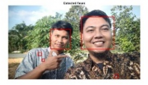
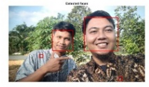
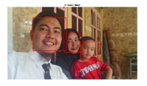
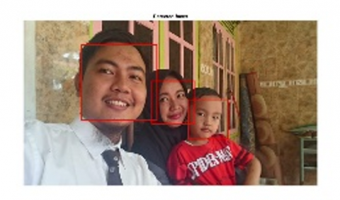
The outcomes of the median and mean filtering are quite important. The outcomes were achieved using median filtering with three criteria from 50 sample photos, the face in the image was recognized in the first 22 samples using TP information, and the second 23 samples with TN information, The third 5 samples with FP description, namely the face in the image, failed to be detected while other objects were discovered, despite the face in the image being detected. The first 21 samples having TP information, which allowed for the detection of faces in images, yielded the best results for mean filtering, the face in the image was detected in the second 24 samples with TN information, although other objects were also detected; the face in the image was not detected in the third 5 samples with FP information. This can happen as a result of the lighting, the object's state at the time of the photo, and the supporting items in the image. Determine the two filtering algorithms' accuracy using the confusion matrix as follows:
$\begin{aligned} \text { accuracy median } & =\frac{T P+T N}{T P+T N+F P+F N}=\frac{22+23}{22+23+5} = \frac{45}{50}=0.9=90 \%\end{aligned}$
$\begin{aligned} \text { accuracy mean } & =\frac{T P+T N}{T P+T N+F P+F N}=\frac{21+24}{22+24+5} =\frac{45}{50}=0.9=90 \%\end{aligned}$
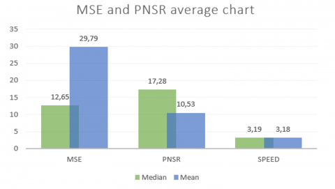
Both filtering techniques have a high accuracy of 90% based on median and mean accuracy, however, as median filtering receives more TP criteria than mean filtering in this instance, it is superior. Figure 5 displays the findings after averaging the MSE and PNSR values.
Figure 5. MSE and PNSR average chart
Based on Figure 5, the average results of MSE and PNSR calculations were obtained from the median and mean filtering methods. If we look at the average of the 50 samples, the lowest MSE score is found in the median filtering method with a value of 12.65, while the highest average PNSR value is also found in the median filtering method with a value of 17.28. The fastest average time was obtained from the mean filtering method with a time of 3.18 seconds. Based on these results it can be concluded that the Median Filtering method is better than the mean filtering method in terms of accuracy and error. Even so, both of these methods can be used and worked well in this study.
This study's result is that, in terms of accuracy and error, the median filtering approach outperforms the mean filtering method. The median filtering method had the lowest average MSE results, with a value of 12.65, and the highest PNSR value, with a value of 17.28, according to the findings of comparing the median and mean filtering methods using MSE and PNSR on 50 image samples. The fastest average time was obtained from the mean filtering method with a time of 3.18 seconds. The accuracy of the median and mean filtering methods, which is 90% based on the confusion matrix, shows that they are effective for face detection scenarios in digital photographs. These two techniques can be used as a guide for face detection because they have both been used successfully to find people in digital photographs.
This research was supported and funded by Institute of Research and Community Services (LPPM) Universitas Ahmad Dahlan, Yogyakarta, Indonesia.
[1] Eleyan, A., Anwar, M. (2017). Multiresolution edge detection using particle swarm optimization. International Journal of Engineering Science and Application, 1(1): 11-17.
[2] Wankhade, M., Wagdarikar, N.M. (2017). Feature extraction of edge detected images. Computer Science, 6(6): 336-345.
[3] Alyushin, M.V., Alyushin, V.M., Kolobashkina, L.V. (2018). Optimization of the data representation integrated form in the viola-jones algorithm for a person’s face search. Procedia Computer Science, 123: 18-23. https://doi.org/10.1016/j.procs.2018.01.004
[4] Deshpande, N.T., Ravishankar, S. (2017). Face detection and recognition using Viola-Jones algorithm and Fusion of PCA and ANN. Advances in Computational Sciences and Technology, 10(5): 1173-1189.
[5] Yudhana, A., Wijaya, S.A. (2022). Penerapan metode median filtering untuk optimasi deteksi wajah pada foto digital. Journal of Innovation Information Technology and Application (JINITA), 4(1): 51-60. http://dx.doi.org/10.35970/jinita.v4i1.1424
[6] Sunardi, S., Yudhana, A., Ardi, S. (2022). Application of mean filtering method for optimizing face detection in digital photos. International Journal of Artifical Intelligence Research, 6(2). https://doi.org/10.29099/ijair.v6i2.307
[7] Kaur, A. (2013). Mingle face detection using adaptive thresholding and hybrid median filter. International Journal of Computer Applications, 70(10): 13-17. https://doi.org/10.5120/11997-7883
[8] Al-Taie, R. (2021). A review paper: Digital image filtering processing. Technium, 3(9): 1-11.
[9] Shaban, S.A., Elsheweikh, D.L. (2022). Blood group classification system based on image processing techniques. Intelligent Automation & Soft Computing, 31(2): 817-834. http://dx.doi.org/10.32604/iasc.2022.019500
[10] Shao, C., Kaur, P., Kumar, R. (2021). An improved adaptive weighted mean filtering approach for metallographic image processing. Journal of Intelligent Systems, 30(1): 470-478. https://doi.org/10.1515/jisys-2020-0080
[11] Choudhary, J., Choudhary, A. (2021). Enhancement in morphological mean filter for image denoising using GLCM algorithm. Interbational Journal of Computer Theory and Engineering, 13(4): 134-137. https://doi.org/10.7763/ijcte.2021.v13.1302
[12] Maharani, S., Ridwanto, H., Hatta, H.R., Dyna, M.K., Ibrahim, M.R. (2021). Comparison of TOPSIS and MAUT methods for recipient determination home surgery. IAES International Journal of Artificial Intelligence, 10(4): 930-937. https://doi.org/10.11591/ijai.v10.i4.pp930-937
[13] Jankowska, K., Ewert, P. (2021). Effectiveness analysis of rolling bearing fault detectors based on self-organising kohonen neural network–A case study of PMSM drive. Power Electronics and Drives, 6(1): 100-112. https://doi.org/10.2478/pead-2021-0008
[14] Balaji, V., Raja, S. (2022). Recommendation learning system model for children with autism. Intelligent Automation & Soft Computing, 31(2): 1301-1315. https://doi.org/10.32604/iasc.2022.020287
[15] Chachlakis, D.G., Zhou, T., Ahmad, F., Markopoulos, P.P. (2021). Minimum Mean-Squared-Error autocorrelation processing in coprime arrays. Digital Signal Processing, 114: 103034. https://doi.org/10.1016/j.dsp.2021.103034
[16] Mehra, R. (2016). Estimation of the image quality under different distortions. Int. J. Eng. Comput. Sci, 5(17291): 17291-17296. https://doi.org/10.18535/ijecs/v5i7.20
[17] Umamaheswari, D., Karthikeyan, E. (2019). Comparative analysis of various filtering techniques in image processing. International Journal of Scientific & Technology Research, 8(9): 109-114.
[18] Abdillah, M.A., Yudhana, A., Fadlil, A. (2021). Compression analysis using coiflets, haar wavelet, and SVD methods. JUITA: Jurnal Informatika, 9(1): 43-48. http://dx.doi.org/10.30595/juita.v9i1.8559
[19] Pambudi, E.A. (2019). Improved Sauvola threshold for background subtraction on moving object detection. International Journal of Software Engineering and Computer Systems, 5(2): 78-89. https://journal.ump.edu.my/ijsecs/article/view/3591, accessed on Jul. 25, 2022.
[20] Senthilkumaran, N., Vaithegi, S. (2016). Image segmentation by using thresholding techniques for medical images. Computer Science & Engineering: An International Journal, 6(1): 1-13. https://doi.org/10.5121/cseij.2016.6101
[21] Kaur, A., Rani, U., Josan, G.S. (2020). Modified Sauvola binarization for degraded document images. Engineering Applications of Artificial Intelligence, 92: 103672. https://doi.org/10.1016/j.engappai.2020.103672
[22] Yudhana, A., Sunardi, S., Saifullah, S. (2017). Segmentation comparing eggs watermarking image and original image. Bulletin of Electrical Engineering and Informatics, 6(1): 47-53. https://doi.org/10.11591/eei.v6i1.595
[23] Li, H., Cao, Y., Wan, Y., Xu, C., Zhang, H., An, H. (2022). An improved temporal phase unwrapping based on super-grayscale multi-frequency grating projection. Optics and Lasers in Engineering, 153: 106990. https://doi.org/10.1016/j.optlaseng.2022.106990
[24] Yoo, J.W., Lee, K.S. (2022). Usefulness of grayscale values measuring hypoechoic lesions for predicting prostate cancer: An experimental pilot study. Prostate International, 10(1): 28-33. https://doi.org/10.1016/j.prnil.2021.11.002
[25] Irgens, P., Bader, C., Lé, T., Saxena, D., Ababei, C. (2017). An efficient and cost effective FPGA based implementation of the Viola-Jones face detection algorithm. HardwareX, 1: 68-75. https://doi.org/10.1016/j.ohx.2017.03.002
[26] Viola, P., Jones, M. (2001). Rapid object detection using a boosted cascade of simple features. In Proceedings of the 2001 IEEE Computer Society Conference on Computer Vision And Pattern Recognition. CVPR 2001, 1: I-I. https://doi.org/10.1109/CVPR.2001.990517
[27] Viola, P., Jones, M.J. (2004). Robust real-time face detection. International Journal of Computer Vision, 57: 137-154. https://doi.org/10.1023/B:VISI.0000013087.49260.fb
[28] Riadi, I., Fadlil, A., Sari, T. (2017). Image forensic for detecting splicing image with distance function. Int. J. Comput. Appl, 169(5): 6-10. http://dx.doi.org/10.5120/ijca2017914729
[29] Zairi, M., Boujiha, T., Ouelli, A. (2021). Improved JPEG image watermarking in data compression domain using block selection strategy. EAI Endorsed Transactions on Internet of Things, 6(24). http://dx.doi.org/10.4108/eai.8-2-2021.168690
[30] Battiato, S., Giudice, O., Guarnera, F., Puglisi, G. (2021). Estimating previous quantization factors on multiple JPEG compressed images. EURASIP Journal on Information Security, 2021(1): 1-11. https://doi.org/10.1186/s13635-021-00120-7
[31] Attaway, S. (2019). Introduction to MATLAB. Elsevier Inc. https://doi.org/10.1016/b978-0-12-815479-3.00001-5, accessed on Nov. 23, 2022.
[32] Vagga, A., Aherrao, S., Pol, H., Borkar, V. (2022). Flow visualization by Matlab® based image analysis of high-speed polymer melt extrusion film casting process for determining necking defect and quantifying surface velocity profiles. Advanced Industrial and Engineering Polymer Research, 5(1): 1-11. https://doi.org/10.1016/j.aiepr.2021.02.003
[33] Coblenz, M. (2021). MATVines: A vine copula package for MATLAB. SoftwareX, 14: 100700. https://doi.org/10.1016/j.softx.2021.100700