Praveenkumar Shermadurai*![]() | Karthick Thiyagarajan
| Karthick Thiyagarajan![]()
© 2023 IIETA. This article is published by IIETA and is licensed under the CC BY 4.0 license (http://creativecommons.org/licenses/by/4.0/).
OPEN ACCESS
A healthy society must take proper measures to handle human stress, a severe health risk. To classify felt mental stress, this work offers an experimental inquiry to determine the proper phase when electroencephalography (EEG) based input from the DEAP dataset is combined with accelerometer sensor data from the WESAD dataset. A multisensory data fusion approach has been proposed to gather complete data for prognostic modeling and analysis. These techniques attempt to create a composite health index (HI) by fusing numerous sensor inputs. To get an aggregated version of the EEG-based data from the DEAP dataset and Accelerometer (ACC) sensor data from the WESAD dataset, we used the k-medoid data aggregation method with time-frame constrained intra-cluster similarity computations. The mental state is then classified into low-stress, medium-stress, and high-stress categories using a CNN trained on this aggregated dataset. Three types of data low stress, medium stress, and high stress, are created. To categorize stress levels, we used three classifiers Support Vector Machine (SVM), Logical Regression (LR), and Naïve Bayes (NB) are used. Three-class stress classification is accurate to 82.85% of the actual value.
stress classification, EEG, accelerometer, WESAD, DEAP, sensors
We are constantly stressed due to how we live and work in today's society. Acute stress is the term used to describe an organism's non-specific response to external stresses for change that put its proficiencies and resources to the test [1]. On the one hand, persistently high acute stress levels reduce human productivity, and the decreased cognitive load may even lead to mistakes in situations requiring precision [2]. However, chronically high-stress levels often negatively affect mental and physical wellness [3]. Consequently, everyone would benefit by periodically evaluating how they handle stress in their daily life. It could be possible to recognize acute stress episodes and initiate proactive or remedial action. Serious accidents may be avoided by seeing high levels of acute stress in persons doing safety-critical duties. However, as it is neither instantly visible nor a single, monolithic idea, accurate stress detection presently faces major hurdles [4].
There are several sorts of stress, and not everyone is inherently harmful. It is good that acute stress is one of the least dangerous kinds of stress because it is also the most common type. We experience acute stress repeatedly throughout the day. Acute stress is brought on by a perceived impending psychological, emotional, or physical threat. A friend fight, a speeding ticket, or passing a test can all lead to acute stress. Whether the threat is real or imagined, the perception of the danger triggers the stress response. Because it happens suddenly and then passes, acute stress is readily controlled. Because it is feasible and relatively fast to recover from acute stress, it doesn't have the same adverse effects on health as chronic stress. Basic relaxation techniques can work rapidly if your stress reaction doesn't resolve into a relaxation response.
For accurate, non-intrusive, and continuous acute stress monitoring, the physiological study of stress levels, which is multimodal and considers several signals, may be utilized [5-8]. Wearable devices can detect stress reactions in real-time, across several modalities, and continuously thanks to wearable and low-power edge computing technologies and machine learning algorithms. Before a stress detection system can be incorporated entirely into wearable technology, some difficulties, such as security, confidentiality, memory utilization, battery backup, and other elements, must be handled. The constrained battery size and form factors that guarantee mobility and wearability have made battery endurance one of the critical downsides of wearable electronics. Furthermore, a wearable multimodal system makes it especially difficult since power-hungry biosensors use a large amount of energy.
The battery life problem in developing machine learning detection algorithms has yet to be addressed explicitly in recent studies on multi-modal monitoring systems [9-11]. These investigations have yet to distinguish the physiological traits that support the models based on energy use. The most beneficial features are selected using conventional feature selection techniques without considering the cost of specific characteristics. They train multimodal machine learning systems to predict output accurately. As a result, they allocate similar weights to elements with miscellaneous expenses and priorities. Nevertheless, in actuality, the edge device's complexity and resource usage are increased by the sensors and biosignal processing algorithms.
In multimodal monitoring systems, three processes require energy to generate a single physiological feature: (1) signal acquisition by the sensors, (2) bio-parameter analysis, which comprises signal processing and segmentation, and (3) extracting features approach. Be mindful that a single signal may provide several bio-parameters and unique characteristics. Once two characteristics from one particular signal are designated, the sensor’s energy cost must be only once, and vice versa if the features come from the exact bio-parameter. The cost of each characteristic is variable and depends on the other options selected.
The EEG is a crucial instrument for detecting stress and has yielded notable results [12] in distinguishing between subjective experiences and stress-related discoveries. EEG is a technique used to monitor and document the electrical activity in the brain [13, 14]. The handling of EEG signals is the most fundamental feature of the current investigation [15]. Numerous approaches have been developed to measure and study stress levels, using a questionnaire or computing the variations in physiological signals. Real-time, online technology called physiological signals enables better stress measurement.
High resolution in the temporal and geographical aspects and high specificity are offered by invasive techniques like local field potential (LFP) with electrocorticography, which fit into two groups: invasive and benign. They only provide a little covering, though, and they might only suit some situations. Currently, noninvasive methods such as functional magnetic resonance imaging (fMRI), electroencephalography (EEG), and magnetic encephalography (MEG) are used to evaluate the effects of stress on human health. EEG and MEG have better resolution than fMRI, which has good spatial resolution but fair temporal resolution.
A controlled setting for measuring stress has been created by Karthick and Manikandan [16]. Three distinct circumstances, including low and high-stress sessions that include sitting, standing, and walking, are engaged in by participants. After that, the accelerometer sensor's activity data and all HRV readings will be collected for stress detection.
The stress classification model may reach excellent accuracy with simple fixed activities and trustworthy stress labels. A controlled environment can offer detailed data for hypothesis testing. Also, it should be noted that this kind of controlled environment cannot easily be applied to real life because there would be various activities, and the information recorded could experience quality issues like incompatible data labels. Because of this, it is still challenging to measure and evaluate felt stress using the data gathered daily.
We classified stress into three stages using the WESAD and DEAP datasets in our tests. For classification, we employed the leave-one-out cross-validation approaches of the support vector machine. Our suggested strategy, the highest among cutting-edge methods, classified three stress states with an average accuracy of 82.85%, to the best of our knowledge.
The following contributions are made via our suggested method: 1) To increase the accuracy of stress classification, we employed hybrid features (EEG and ACC characteristics generated from our intended trials) from the DEAP and WESAD datasets. 2) Out of 32 EEG electrodes, we chose four (FP1, FP2, F3, and C4) using K-Medoid clustering as the best fit for the classification task. 3) Among cutting-edge techniques, our suggested model distinguished between three different stress levels with the most significant degree of accuracy.
Acute stress events cause a physiological response in the body known as the stress response, which causes several activities coordinated by the autonomic nervous system, such as skin perspiration, increased heart rate, and increased breathing frequency. Wearable sensors can assess these reactions on a variety of physiological signals, including skin temperature (SKT), electrodermal activity (EDA), and respiration (RSP) [17]. A reliable acute stress prediction has been demonstrated to need fused data from many modalities (signals) [18, 19].
However, because of memory, energy use, and duty cycle limitations, multimodal machine-learning techniques are challenging to implement on wearable devices. Even yet, edge computing (also known as edge processing) still has advantages over cloud computing for these multimodal regards to transmission expenses, data protection and privacy, and battery life [20-25]. Instead of developing a cost-aware machine-learning model, substantial effort has been put into making hardware platform improvements (sensor systems and micro-controllers) [26-30] to get around these restrictions. Prior studies have typically intensive on simplified models and limited characteristics. All characteristic costs are assumed to be the same without accounting for how much they vary in costs [31, 32].
The goal of several investigations has been to identify stress automatically. To identify behavior associated with user stress levels, smartphone accelerometer data is employed [33, 34]. The workplace is a significant area in which stress sensing is used. Hernandez et al. tracked the facial temperature using a thermal infrared camera and looked at how it related to stress levels [35]. Koldijk et al. [36] created artificial classifiers to analyze sensor data, including body postures, facial expressions, computer logs, and physiological data, to study the association between working circumstances and conditions associated with mental stress (ECG and skin conductance). This freely accessible WESAD dataset has been the subject of several investigations. In one such work, stress is automatically recognized using various machine learning techniques on the WESAD Dataset while utilizing a variety of statistical variables [37].
Cinaz et al. [38] gave the contributors to prepare and present on an unspecified topic and categorized the felt stress into three groups using the findings from the perceived stress scale (PSS) feedback form. Similarly, Healey and Picard [39] designated three goal stress levels based on the stress ratings from the PSS questionnaire. Chen et al. [40] employed a mental arithmetic task with three levels of difficulty to alter the cortical brain processes that were afterward captured by EEG data. The three test categories were used to categorize the features that cause stress. The study compared the three stress levels caused by mental arithmetic exercises and found that the Alpha power considerably decreased from the first to the second stress level. But the power increased once again from the second to the third level. This information also supports the conclusion that cortical activation was unsuccessful at task level three.
In the study [41], Castaldo et al. employed a variety of sensors to identify stress, including video, knee-mounted accelerometers, galvanic skin reactions, and cardiac sensors. Their findings demonstrated that integrating behavioral data in addition to physiological measurements increased the accuracy of stress identification compared to utilizing only physiological features. There has also been a recent study on employing wearable sensors to detect stress outside of lab settings. An application that runs on a smartphone was developed by Gjoreski et al. [42] to identify stress via voice input. Bogomolov et al. [43] classified stressed and not stressed states using data from a wrist sensor, questionnaires, and mobile phones, with more than 75% accurate findings.
It is acknowledged that the amount of stress experienced by people in this setting differs from stress in everyday life. Additionally, it has been shown that people dislike using intrusive measuring equipment and find them uncomfortable. These reasons have prompted researchers studying stress to look beyond the lab and develop a non-intrusive multi-level stress monitoring system. Due to their widespread use in current society, cell phones and wearable technology have been selected as tools for stress detection in daily Sensors. After laboratory settings, research on stress level detection has been done in confined and semi-confined spaces, including offices, cars, and college campuses. Workplaces and offices are among the settings where stress levels are most elevated.
EDA, ECG (Electrocardiogram), and accelerometer are used to measure stress levels in the workplace. Individual’s stress levels rise amid traffic congestion, especially in populated cities. There are several studies in the literature about driving environments. Drive DB database was utilized in the majority of investigations. This database contains data from 24 Boston drivers' ECG, EDA, EMG (Electromyogram), and breathing sensors.
When researchers applied machine learning techniques to this data, the EDA-ECG signal combinations and Classifier performed best. Campus environments are the closest to free everyday life environments since they are semi-restricted. As a result, classification performances could be better compared to constrained laboratory, office, and automotive contexts. The decision tree classifier with an ECG signal had the most significant classification accuracy in a campus setting for two-class categorization [44]. The majority of works have solely utilized smartphone functionality. Most of the work needs to use intelligent wearables on campuses.
However, chronically high-stress levels might have a more significant negative impact. A state of chronic stress is one in which the body's stress response is continuously elicited. Chronic stress can result from either repeated happening of similar acute stressors (experiencing the very same stress repeatedly) or multiple instances of different acute stressors (a sequence of unrelated stressful situations). Because of this, having a stress management strategy is crucial.
A person's individual, social, and cultural health are all significantly impacted by the current field of study in stress detection and monitoring. The current methods for classifying emotional states use conventional machine-learning techniques and characteristics calculated from various sensor modalities. These techniques need many data and rely on handmade traits, which makes it difficult to utilize these sensor systems in daily life. To address these issues, we provide a new Neural Network Model-based stress recognition and classification framework that uses input from many sensor modalities without doing any feature computation. Our approach is competitive, surpasses the most advanced methods currently available, and obtains an accuracy of classification of 82.85%.
3.1 DEAP and WESAD
The DEAP dataset [45] includes multimodal measures, including video recordings, EEG, and external physiological responses, made using commercially available equipment during 16 sessions of around 10-minute-long paired conversations on a social problem. It varies from past datasets in that it includes emotional assessments from the perspectives of the debater, the other participant, and the audience. Every five seconds while they watched the debate film, raters noted emotional outbursts in terms of physiological and 18 other category emotions.
All subjects' EEG data was gathered while they watched films. There were 40 movies displayed, each of which had a unique ID and covered a distinct genre. Every participant saw a series of 60-second films that were played in order. There are two signal arrays in the EEG electrode data: 1) The data array (40 40 8064) indicates that a user watched 40 films and that 8064 data samples were gathered from 40 EEG channels. 2) For each movie, there are four goal labels in the second array: valence, arousal, dominant, and liking.
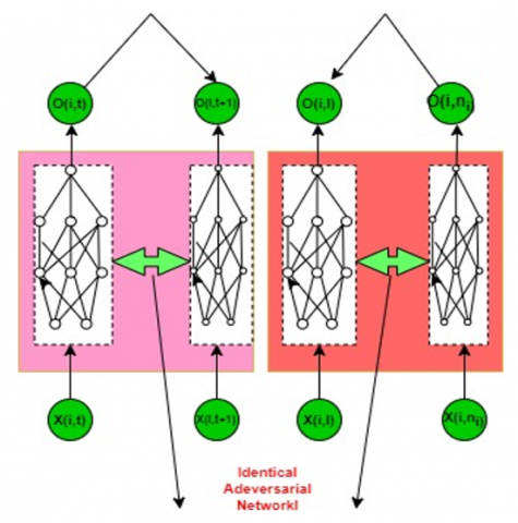
Figure 1. Data fusion construct
This study made use of the WESAD dataset. Attila Reiss et al. originally made this dataset available to the general public in 2018 [46]. Fifteen patients' movements and physiological data were recorded using the RespiBAN Advance chest apparatus and the Empatica E4 arm sensor. The physiological reactions of the subjects were recorded using the following study techniques: baseline, getting ready, having fun, having stress, meditating, and recovering. The specifications of the sensor setup, position, and methodology used to produce this collection of data, as well as the data obtained throughout each patient research process, are provided in Ref. [47]. The heart rate, ACC, Respiration (RESP), Electromyography signals (ECG), Temperature (TEMP), and RESP were all measured using RespiBAN. All signs were captured at a frequency of 700 Hz. E4 was used to record the TEMP, RESP, ACC, and Electrocardiogram signals at various frequencies, including 3.5ghz, 8 Hz, 16 Hz, 32 Hz, and 64 Hz.
All sensor signals were divided up using the sliding window approach. These traits fit within the group described in the study [48]. To add the absolute values of the three axes on the unprocessed ACC signal, several statistical metrics, such as mean, mode, standard deviation, median, minimum, and maximum, were individually determined for the x, y, and z axes. Statistics were created using the unprocessed ACC, RESP, ECG, and TEMP data, including mean, mode, median, standard deviation, minimum, and maximum values. We calculated statistical metrics such as mean, standard deviation, mode, lowest, median, and maximum values from the raw measurements from the accelerometer, respiration, electrocardiogram, and temperature sensors. It uses TEMP, TEMP optimal rate, and signal gradient as characteristics. Statistical parameters such as the mean, standard deviation, lowest value, and maximum value were retrieved [49] after the raw ECG signal was filtered through a low-pass filter with a frequency of 5 Hz.
3.2 Data fusion
The top layer receives the input, while the bottom layer gives the output. The intermediate tiers are called hidden layers because they are hidden from the outside world. A layer's perceptron is all connected to those in the layer above it. This is how the feed-forward network gets its name—data feeds continually from one unit to the next. In the same layer, the perceptron is not coupled. No feedback loop connects the current layer to the layer above it. The perceptron is the fundamental neural network unit that establishes the weighted sum of the input values.
The mathematical mapping y = f (x: θ) is created using a feed-forward neural network to get the best function approximation and learn the parameter’s value. A feed-forward neural network has bias units in each unit beside the output unit. Biases play a crucial role in effective learning by shifting the activation function to the left or the right. The following parameters apply to a feed-forward neural network with a single hidden unit, as shown in Eq (1).
(i × h + h × o) + h + o (1)
i - number of neurons in the input layer.
h - number of neurons within the hidden layer.
o - number of neurons in the output layer.
A DNN-based data fuse model, as seen in Figure 1, defines a nonlinear projection from an original input to the HI space as $f: X \in R^s \rightarrow O \in R$, where S is the total number of the sensors under consideration. Figure 1 shows a feed-forward network with one input and output unit and two hidden units. We use the following Eq. (2) to receive the numerous sensor signals.
h0 = [Xi, j] = [Xi,1, Xi, s, …., Xi, j] (2)
h0 is the number of neurons allocated to the input unit.
The HIs are supposed to have continuous values, making this work a regression problem. We gave the output unit an h0 value of 1. Each neuron in the hidden units and the output unit represents a composite function as a convolution followed by a sigmoid activation transformation. Let Pj define the number of neurons at unit j, and j represents the number of hidden units. Zij means the sequential result of component i at unit j, and the sigmoid transformation function is indicated by Eq. (3).
$\mathrm{Z}_{\mathrm{ij}}=\left(w_i^j\right) \mathrm{h}_{1-1}+\mathrm{b}_{\mathrm{ij}} ; w_i^j=\left[w_{1 i}^j, \ldots, w_{p_{l-1} \,\,i}^j\right]^{\prime}$ (3)
The weight $\boldsymbol{R}^{\prime p_{l-1}}$ denotes the connection between unit j's neuron i's input and unit j's output.
here, hl−1 =$\left[\boldsymbol{h}_1^{l-1}, \ldots, \boldsymbol{h}_{p_\,{l-1}}^{l-1}\right]^{\prime} \in \mathbf{R}^{p_{l-1}}$.
where bij is the bias of neuron i at unit j.
Each neuron's sigmoid transformation function output is supplied into a nonlinear transformation function. We have activated neurons using the sigmoid function defined in Eq. (4).
$h_i^l=\omega\left(z_i^l\right)=\frac{1}{1+e^{-z_i^l}}$ (4)
Suppose Zo = (Wo)’ hL + bo and Wo = ω(Zo) are the weight connecting the final hidden unit to the output unit.
hL = $\left[h_1^L, \ldots, h_{p_L}^L\right]^{\prime} \in \mathbf{R}^{p_L}$ are input to the hidden unit and bo is the bias of the output unit.
Wo = $\left[\mathbf{W}_1^o, \ldots, \mathbf{W}_{p L}^o\right]^{\prime} \in \mathbf{R}^{p l}$ indicate the output mapping that is linearly transformed and nonlinearly mapped.
The DNN-based batch learning method, which handles the unsupervised learning issue, incorporates the chosen attributes. It is presented by using many unlabeled sensors, a vital task following the construction of the CNN architecture for HI. The objective function is created by fusing these two characteristics using the tuning parameter $\lambda_1 \in(0,1)$ as in Eq. (5).
λ1 ∗ Mono + (l – λl) ∗ R (5)
We view the optimization problem as a system of various antagonistic terms, that is $\operatorname{Mono}_{i, j}$ and range parameters, Ri, which are the essential units for model development. To incorporate these qualities in the architecture. However, because there are many more monotonic parameters $\sum_{i=1}^m\left(n_i-\mathbf{m}\right)$ than range parameters ‘m’, using each of them as a training data separately would result in a skewed sampling issue during combinational optimization. To solve this problem, each range parameter Ri is split into ( $n_i$ − m) subrange parameters 1/ ( $n_i$−m) ∗ Ri, and each of these is then combined with the monotone term's opposite, which is 1.
$\lambda_1 * \operatorname{Mono}_{i, \mathrm{j}}+\frac{\left(1-\lambda_1\right)}{n_i-1} * R_i=\lambda_1 c_{i, \mathrm{j}} * \max \left(o_{i, \mathrm{j}}-o_{i, \mathrm{j}+1}, \alpha\right)+\frac{\left(1-\lambda_1\right)}{n_i-1} *\left(o_{i, n_i}-o_{j, 1}-\beta\right)^2$ (6)
In Eq. (6), $\operatorname{Mono}_{i, j}$ gives the atomic term for unit i at time j, and Ri is the range parameter for unit i.
The resulting design, depicted in Figure 1, incorporates two adversarial networks related to the monotonic properties and range characteristics. This implies that these two interconnected systems attempt to change the attributes of DNN during training operations by combining them with similar parameters.
To determine if the periodicity and range properties are met, the outcomes of each pair of units are evaluated explicitly to one another at each phase. If these requirements are not satisfied, the number of mistakes is calculated and sent back to change the model parameters. In this way, errors are continuously reduced until convergence.
A pair of facts linked to sparsity, [Xi, j, Xi, j+1] ∈ $R^{s \times 4}$, and a pair of points related to the range, $\left[\mathrm{X}_{i, n_i}, \mathrm{X}_{\mathrm{i}, 1}\right] \in R^{s \times 4}$, establish two different forms of adversarial connections that, practically speaking, enable DNN learning. Monotonicity is initially offered as an instance of this.
These systems may now use an adversarial strategy due to the sparsity of two nearby outputs, $o_{i, \mathrm{t}}$ and $o_{i, \mathbf{t}+1}$. To be more specific, as shown in the left side of Figure 1, two similar systems for $o_{i, j}$ and $o_{i, j+1}$ compete with one another during learning till monotonicity is fulfilled i.e., $o_{i, j} \leq o_{i, j+1}$ or the breach of sparsity is minimized that is min {max ( $o_{i, j}, o_{i, j+1}$, α)}.
Related to this, the range property conflicts with the starting points $o_{i, 1}$ and $\boldsymbol{o}_{i, n_i}$ for component i, as seen on the right side of Figure 1. Particularly, two similar systems linked to $o_{i, 1}$ and $o_{i, n_i}$ collide with one another unless the range traits are fulfilled, or the breach of the range limitation is reduced, that is, min {max ( $o_{i, j}, o_{i, j+1}$, α)}.
For stochastic optimization, they are combined to form a training sample, as in Eq. (7).
$\mathrm{X}_{i j}^k=\left[\mathrm{X}_{\mathrm{i}, \mathrm{j}}, \mathrm{X}_{\mathrm{i}, \mathrm{j}+1}, \mathrm{X}_{i, n_i}, \mathrm{X}_{\mathrm{i}, 1}\right], \mathrm{k} \in R^{s \times 4}$ (7)
where k =1 to $\sum_{i=1}^m\left(n_i-\mathrm{m}\right)$ is the sample index in the dataset.
$\operatorname{Mon}_{i j}^k=\operatorname{Mon}_{i, \mathrm{j}}, R_{i j}^k=R_i$, and $c_{i j}^k=\boldsymbol{c}_{i, j}$ (8)
As a result of Eq. (8), we got $o_{i j}^k=\left[o_{i, j}, o_{i, j+1}, o_{i, n_i}, o_{i, 1}\right]^k \equiv\left[o_{i, j}^k, o_{i, j+1}^k, o_{i, n_i}^k o_{i, 1}^k\right] \in \mathbf{R}^{1 \times 4}$, in which $o_{i, j}$ is the constructed HI of unit i at time j.
3.3 The organizational structure of CNN
We employ a deep CNN structure to assess the patch that represents the signal frames point and obtain the interest of points description of the signals [50]. The seven convolution layers that makeup CNN, are seen in Figure 2, have three convolutional layers with a 4*4 kernel and three pooling layers with a 2*1 kernel. A pooling layer follows each convolution layer.
The convolutional layers use a series of kernels to automatically generate the extracted features that serve as the input to the subsequent layers. An approximation technique called Rectified Linear Unit further purges the feature maps (ReLU). Pooling eliminates the weak components and reduces the feature dimension while preserving the critical characteristics of a kernel.
To prevent the CNN architecture from progressing gradually or modifying the distribution of data provided to the active layer throughout the training phase, backpropagation is used. The network's contouring will disappear if backpropagation is utilized, slowing down data transport during training. At the same time, the issue of over-fitting may be managed, as well as the case of the convolution network being sensitive to the activation weight.
The bias vector known as the Rectified Linear Unit (ReLu) does nonlinear operations on extracted features that have undergone batch regularization. The expression of the function is given as in Eq. (9).
H(x)=max(0, x) (9)
Due to the Relu function's unilateral suppression, the CNN can activate sparsely, better visual features, better-fit training data, and recognize more expressions. The Dropout layer, which follows the sixth ReLu layer, seeks to lessen the network's over-fitting issue while lowering the coupling between various parameters.
The Dropout layer is only used once since this convolutional neural network topology uses BN layers, which can help alleviate the overfitting issue. After feature extraction, we combine these two categories of characteristics to obtain the fusion features. To develop more discriminative features, feature fusion integrates the features obtained from the sensor- and vision-based techniques. A Random Forest classifier uses the recovered attributes to determine whether or not the subject is stressed.
Figure 2. Overall proposed system model
3.4 CNN for feature extraction
The CNN model has seen much success in image processing. To obtain features, CNN learns the convolution in each convolution layer. Methods including dimension reduction and multi-layer convolutional kernel operations are applied to extract image data from the input image. The predicted data is received by sharing the CNN model's layer information while the model is trained. Backpropagation is used to transmit the difference in values between the observed and predicted values, and the loss function is used to send the fractional derivative of each layer's parameter. The gradient descent technique is used to update each layer's parameters. The network can remarkably describe the picture since it continuously learns and changes its parameters. We employed a deep neural network structure in this study. A multi-layer convolution network improves the extraction accuracy of the description of visual characteristics. To improve the network's resilience, the triple loss function was utilized for training the network, and the stochastic gradient descent technique was used to update the parameters.
3.5 K-medoid
Algorithm 1: K-Medoid
Input: WESAD and DEAP dataset,
Result: Medoids M
1. Pick k objects at random to serve as initial medoids.
2. Give the closest medoids to each of the remaining objects.
3. The sum of all item differences from the closest medoid is the aim function, which should be found.
4. Use Oramdom to choose a non-medoid object at random.
5. If objective performance was enhanced, then Switching Oramdom and O.
6. Calculate the total cost of the trade.
7. Continue iterating steps 3 through 6 until there is no change.
To decrease this study’s data, we apply the k-medoids clustering approach. An input for n observations is divided into k clusters using the "K-Medoids Clustering" method, with each data point matching the cluster that contains the nearest medoid. The k-Means and medoid algorithms are combined to accomplish this. One might use the object or medoids positioned in the cluster’s center instead of utilizing the average value of the cluster's elements. A data point is recognized as the medoid out of a finite data collection if its mean differentiation to all other sample points is below a particular threshold. In terms of execution speed and susceptibility to outliers or noise, it improves k-means clustering.
3.6 Classification models
In this study, y = [low stress, medium stress, or high stress] was used to simulate the link between the reduced set of attributes and the related treatment response (low stress, medium stress, or high stress) by Eq. (10) [51]. The coefficient calculations for the LR classifier were based on the maximum likelihood strategy. A probability score p(x), where 0 ≤ p(x) ≤ 1, was produced by the LR classifier and indicated whether the condition was related to stress or control. The condition was classified as stress if p(x) was more than the threshold value of 0.5.
$F(z)=E(Y / x)=\frac{1}{1+e^{-z}}$ (10)
In Eq. (10), Y is the class label given low, medium, or high-stress values. Additionally, x is a synthesis of various qualities. We utilized the logistic function and the formula z = α + β1X1 + β2X2 + ,..., + βkXk to derive the LR model. Eq. (11) represents the logistic function by altering the value of z from Eq. (10).
$F(z)=E(Y / x)=\frac{1}{1+e^{-\left(\alpha+\sum \beta_i X_i\right)}}$ (11)
The probability that an individual will respond or not is determined and represented by the letters Y or p(x). The LR classifier generated a chance of p(x), which meant whether the individuals belonged to the stressful or control categories, where 0<p(x) ≤ 1. Low stress has deemed the condition if p(x) was more than the threshold value of 0.5. When p(x) exceeded the threshold value of 0.7, the state was classified under "medium stress." When p(x) exceeded the threshold value of 0.85, the state was classified as under "high stress."
The Classification models with such a sigmoid kernel were utilized as the second classifier. According to the class labels, the feature space might be divided into stress and control scenarios using a "hyperplane.” The SVM, a more advanced classification model, is used for comparison. The SVM claims a linear decision boundary may be discovered based on this high-dimensional space. The risk of over-fitting the data decreased, our data performed substantially better, and the total model complexity was significantly lowered using a linear kernel instead of a nonlinear kernel. In conclusion, the SVM created a hyperplane to obtain the highest level of classification accuracy, while the LR classifier provided probability values to categorize stress.
The Naïve Bayes classifier, which is reliant on producing the conditionally posterior probability of each sample when incorporating the target condition, stress vs. control, is the third classification model. The classifier was created by categorizing the sample in the category with a greater posterior probability.
The three-level stress SVM classification's performance and prediction results are summarized in the confusion matrix, which is displayed in Table 1. Low-level stress circumstances were appropriately identified as actual occurrences from the low-stress class. This amounted to 43% of all 50 occurrences, and 100% of those instances were correctly classified into the relevant category.
Regarding the moderate stress level, 25 instances that made up 54% of the total were correctly classified, and the overall percentage of correct classification for that specific class was 100%. Only one of the eight highly stressed predictions (1 actual incidence) from the highlight stresses was misclassified as moderate stress, which accounted for 2% of all cases (i.e., seven instances) or 14% of the highly stressed predictions. The confusion matrix shows that the three-level stress categorization often provided 82% correct predictions and 18% wrong ones.
Table 1. Confusion matrix of three-class stress level of SVM classifier
|
Low |
Medium |
High |
|
|
Low |
1343 |
863 |
193 |
|
Medium |
585 |
3710 |
541 |
|
High |
26 |
245 |
7003 |
Table 2. Stress classification accuracy
|
Algorithm |
Accuracy |
||
|
ACC |
EEG |
ACC+EEG |
|
|
LR |
68.98 |
71.59 |
76.85 |
|
SVM |
60.46 |
72.09 |
80.09 |
|
NB |
62.79 |
69.76 |
75.93 |
From Table 2, the SVM algorithm attained a maximum classification accuracy of 85.62% for 2-class and 80.09% for 3-class using ACC and EEG inputs. The EEG signal obtains greater detection accuracies with all methods, which is another significant observation. Maximum accuracy rises to 89.04% for 2-class and 80.54% for 3-class classification, especially when the features are combined with time and frequency domain features and feature selection is used.
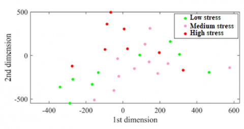
Figure 3. Graphical visualization of features selected for perceived stress classification
The traits selected using our recommended method for stress classification are shown in Figure 3 in two dimensions using the t- Stochastic Neighbor Embedding scheme(t-SNE) [52], a dimension reduction approach to depicting high dimensional data. We discovered that the two classes that are stressed and non-stressed are easier to differentiate from the three classes visually. This demonstrated that the chosen criteria successfully discriminated between perceived stress groups with two and three classes.
Figure 4. The density function for entropy features
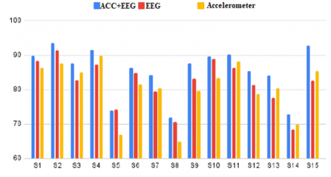
Figure 5. Stress classification accuracy of using accelerometer and EEG data
Figure 4 displays the entropy feature's estimated distribution for all users. Vertical lines represent the median. Visual inspection reveals that the median Entropy of high and mild stress differs. Although less pronounced than the difference between medium and low stress, the gap between high and moderate stress is perceptible. Entropy appears to be a strong candidate trait for separating high/low and medium/low-stress levels, but it may have trouble separating high/medium stress levels.
Figure 5 shows the model’s accuracy on ACC+EEG data, ACC data for each subject, and only EEG data for each subject. Compared to EEG or ACC, which had accuracy values of 72.09% and 68.98%, respectively, it was shown that ACC+EEG predicted the stress condition more accurately. However, both methods performed poorly compared to combined data (EEG and ACC), which produced an accuracy value of 80.09%.
In this work, the underlying IoMT-based WESAD dataset and the DEAP dataset for mental health were condensed to train a CNN model. The cumulative edition of the WESAD dataset was built using k-medoid cluster analysis. However, due to the k-scalability medoid's concerns, we limited the intra-cluster similarity calculations using a time-frame window and reduced the processing cost. The overall execution time was shortened using the data clustering approach.
Further study can take advantage of the modalities employed in conjunction with physiological parameters such as facial expression, logging records, audio or video recordings, etc., and a new dataset can be presented. Such a dataset can be utilized for stress classification with higher accuracy because it contains almost all the features needed to cause stress in humans.
[1] Selye, H. (1950). Stress and the general adaptation syndrome. British Medical Journal, 1(4667): 1383-1392. https://doi.org/10.1136/bmj.1.4667.1383
[2] Schneiderman, N., Ironson, G., Siegel, S.D. (2005). Stress and health: Psychological, behavioral, and biological determinants. Annual Review of Clinical Psychology, 1: 607-628. https://doi.org/10.1146/annurev.clinpsy.1.102803.144141
[3] Epel, E.S., Crosswell, A.D., Mayer, S.E., Prather, A.A., Slavich, G.M., Puterman, E., Mendes, W.B. (2018). More than a feeling: A unified view of stress measurement for population science. Frontiers in Neuroendocrinology, 49: 146-169. https://doi.org/10.1016/j.yfrne.2018.03.001
[4] Alberdi, A., Aztiria, A., Basarab, A. (2016). Towards an automatic early stress recognition system for office environments based on multimodal measurements: A review. Journal of Biomedical Informatics, 59: 49-75. https://doi.org/10.1016/j.jbi.2015.11.007
[5] Montesinos, V., Dell'Agnola, F., Arza, A., Aminifar, A., Atienza, D. (2019). Multi-modal acute stress recognition using off-the-shelf wearable devices. Annual International Conference of the IEEE Engineering in Medicine and Biology Society (EMBC), Berlin, pp. 2196-2201.
[6] Momeni, N., Dell'Agnola, F., Arza, A., Atienza, D. (2019). Real-time cognitive workload monitoring based on machine learning using physiological signals in rescue missions. Annual International Conference of the IEEE Engineering in Medicine and Biology Society (EMBC), Berlin, pp. 3779-3785.
[7] Zhang, H.H., Zhu, Y.W., Maniyeri, J., Guan, C. (2014). Detection of variations in cognitive workload using multimodality physiological sensors and a large margin unbiased regression machine. Annual International Conference of the IEEE Engineering in Medicine and Biology Society, Chicago, pp. 2985-2988.
[8] Arza, A., Garzón-Rey, J.M., Lázaro, J., Gil, E., Lopez-Anton, R., de la Camara, C., Laguna, P., Bailon, R., Aguiló, J. (2019). Measuring acute stress response through physiological signals: Towards a quantitative assessment of stress. Medical & Biological Engineering & Computing, 57(1): 271-287. https://doi.org/10.1007/s11517-018-1879-z
[9] Song, C., Liu, K., Zhang, X. (2018). Integration of data-level fusion model and kernel methods for degradation modeling and prognostic analysis. IEEE Transactions on Reliability, 67(2): 640-650. https://doi.org/10.1109/TR.2017.2715180
[10] Kim, M., Song, C., Liu, K. (2019). A generic health index approach for multisensor degradation modeling and sensor selection. IEEE Transactions on Automation Science and Engineering, 16(3): 1426-1437. https://doi/10.1109/TASE.2018.2890608
[11] Woaswi, W., Hanif, M., Mohamed, S.B., Hamzah, N, Rizman, Z.I. (2016). Human emotion detection via brain waves study by using electroencephalogram (EEG). International Journal on Advanced Science, Engineering and Information Technology, 6(6): 1005-1011. http://dx.doi.org/10.18517/ijaseit.6.6.1072
[12] Preethi, J. Sreeshakthy, M., Dhilipan, A. (2014). A survey on EEG-based emotion analysis using various feature extraction techniques. International Journal of Science, Engineering and Technology Research (IJSETR), 3(11).
[13] Saidatul, M.P. Paulraj, S. Yaacob, Yusnita, M.A. (2011). Analysis of EEG signals during relaxation and mental stress condition using AR modeling techniques. Proceedings of the IEEE International Conference on Control System, Computing and Engineering, Penang. http://dx.doi.org/10.1109/ICCSCE.2011.6190573
[14] Deshmukh, R., Deshmukh, M. (2014). Mental stress level classification: A review. International Journal of Computer Applications, 1: 15-18.
[15] Sun, F.T., Cynthia, K., Cheng, H.T., Buthpitiya, S., Collins, P., Griss, M.L. (2012). Activity-aware mental stress detection using physiological sensors. Mobile Computing, Applications, and Services, pp. 211-230. http://dx.doi.org/10.1007/978-3-642-29336-8_12
[16] Karthick, T. Manikandan, M. (2018). Fog-assisted IoT-based medical cyber system for cardiovascular diseases affected patients. Concurrency and Computation: Practice and Experience, 31: e4861. https://doi.org/10.1002/cpe.4861
[17] Betti, S., Lova, R.M., Rovini, E., Acerbi, G., Santarelli, L., Cabiati, M., Del Ry, S., Cavallo, F. (2018). Evaluation of an integrated system of wearable physiological sensors for stress monitoring in working environments by using biological markers. IEEE Transactions on Biomedical Engineering, 65(8): 1748-1758. https://doi.org/10.1109/TBME.2017.2764507
[18] Sharma, N., Gedeon, T. (2014). Modeling a stress signal. Applied Soft Computing, 14: 53-61. https://doi.org/10.1016/j.asoc.2013.09.019
[19] Karthick. T. (2020). Emotion detection and therapy system using Chatbot. International Journal of Advanced Trends in Computer Science and Engineering, 9: 5973-5978. 10.30534/ijatcse/2020/263942020
[20] Dell’Agnola, F., Momeni, N., Valdés, A.A., Atienza, D. (2020). Cognitive workload monitoring in virtual reality-based rescue missions with drones. Virtual, Augmented and Mixed Reality, pp. 397-409. http://dx.doi.org/10.1007/978-3-030-49695-1_26
[21] Golgouneh, A., Tarvirdizadeh, B. (2020). Fabrication of a portable device for stress monitoring using wearable sensors and soft computing algorithms. Neural Computing and Applications , 32(11): 1-23. https://link.springer.com/article/10.1007/s00521-019-04278-7
[22] Sopic, D., Aminifar, A., Aminifar, A., Atienza, D. (2018). Real-time event-driven classification technique for early detection and prevention of myocardial infarction on wearable systems. IEEE Trans. IEEE Transactions on Biomedical Circuits and Systems, 12(5): 982-992. https://doi.org/10.1109/tbcas.2018.2848477
[23] Surrel, G., Aminifar, A., Rincon, F., Murali, S., Atienza, D. (2018). Online obstructive sleep apnea detection on medical wearable sensors. IEEE Transactions on Biomedical Circuits and Systems, 12(4): 762-773. https://doi.org/10.1109/tbcas.2018.2824659
[24] Bharathi, A, Natarajan A.M. (2010). Cancer classification of bioinformatics data using ANOVA. International Journal of Computer Theory and Engineering, 2(3): 369-373. http://dx.doi.org/10.7763/IJCTE.2010.V2.169
[25] Witten, I.H., Frank, E., Hall, M.A. (2011). Data mining: Practical machine learning tools and techniques, 3rd ed., ser. The Morgan Kaufmann Series in Data Management Systems. Elsevier Science. http://books.google.com.mx/books?id=5FIEAwyn9aoC, accessed on Sept. 22, 2022.
[26] Chiesa, A., Serretti, A. (2010). A systematic review of neurobiological and clinical features of mindfulness meditations. Psychological Medicine, 40(8): 1239-1252. https://doi.org/10.1017/s0033291709991747
[27] Burges, C.J.C. (1998). A tutorial on support vector machines for pattern recognition. Data Mining and Knowledge Discovery, 2(2): 121-167. http://dx.doi.org/10.1023/A:1009715923555
[28] Critchley, H.D. Tang, J., Glaser, D., Butterworth, B., Dolan, R.J. (2005). Anterior cingulate activity during error and autonomic response. NeuroImage, 27(4): 885-895. https://doi.org/10.1016/j.neuroimage.2005.05.047
[29] Maaten, L.V.D., Hinton, G.E. (2008). Visualizing data using t-SNE. Journal of Machine Learning Research, 9(11): 2579-2605.
[30] Garcia-Ceja, E., Osmani, V., Mayora, O. (2015). Automatic stress detection in working environments from smartphone’s accelerometer data: a first step. IEEE Journal of Biomedical and Health Informatics, 20(4): 1053-1060. https://doi.org/10.1109/jbhi.2015.2446195
[31] Ishimaru, S., Kise, K. (2015). Quantifying the mental state on the basis of physical and social activities. In Adjunct Proceedings of the 2015 ACM International Joint Conference on Pervasive and Ubiquitous Computing and Proceedings of the 2015 ACM International Symposium on Wearable Computers, Sakai, pp. 1217-1220. https://doi.org/10.1145/2800835.2807934
[32] Hoffmann, S., Tauscher, H., Dengel, A., Ishimaru, S., Ahmed, S., Kuhn, J., Heisel, C., Arakawa, Y. (2016). Sensing thermal stress at office workplaces. In Proceedings of the 5th International Conference on Human-Environment Systems, ICHES 2016, Nagoya, pp. 25.
[33] Bobade, P., Vani, M. (2020). Stress detection with machine learning and deep learning using multimodal physiological data. In 2020 Second International Conference on Inventive Research in Computing Applications (ICIRCA), Coimbatore, pp. 51-57.
[34] Picard, R.W. (2016). Automating the recognition of stress and emotion: From lab to real-world impact. IEEE MultiMedia, 23(3): 3-7. https://doi.org/10.1109/MMUL.2016.38
[35] Hernandez, J., Morris, R.R., Picard, R.W. (2011). Call center stress recognition with person-specific models. In Affective Computing and Intelligent Interaction-Volume Part I, Proceedings of the 4th International Conference on Affective Computing and Intelligent Interaction, Memphis, Germany, pp. 125-134.
[36] Koldijk, S., Sappelli, M., Verberne, S., Neerincx, M., Kraaij, W. (2014). The SWELL knowledge work dataset for stress and user modeling research. Proceedings of the 16th International Conference on Multimodal Interaction, Istanbul, Turkey, pp. 291-298. https://doi.org/10.1145/2663204.2663257
[37] Okada, Y., Yoto, T.Y., Suzuki, T., Sakuragawa, S., Sugiura, T. (2013). Wearable ECG recorder with acceleration sensors for monitoring daily stress: Office work simulation study. International Conference on IEEE Engineering in Medicine and Biology Society (EMBC), Osaka, pp. 4718-21. https://dopi/10.1109/EMBC.2013.6610601
[38] Cinaz, B., Arnrich, B., Marca, R., Tröster, G. (2013). Monitoring of mental workload levels during an everyday life office-work scenario. Personal and Ubiquitous Computing , 17: 229-239.
[39] Healey, J.A., Picard, R.W. (2005). Detecting stress during real-world driving tasks using physiological sensors. IEEE Transactions on Intelligent Transportation Systems, 6(2): 156-166. http://dx.doi.org/10.1109/TITS.2005.848368
[40] Chen, L.L., Zhao, Y., Ye, P.F., Zhang, J., Zou, J.Z. (2017). Detecting driving stress in physiological signals based on multimodal feature analysis and kernel classifiers. Expert Systems with Applications, 85(1): 279-291. https://doi.org/10.1016/j.eswa.2017.01.040
[41] Castaldo, R., Xu, W., Melillo, P., Pecchia, L., Santamaria, L., James, C. (2016). Detection of mental stress due to oral academic examination via ultra-short-term HRV analysis. In Proceedings of the 2016 38th Annual International Conference of the IEEE Engineering in Medicine and Biology Society (EMBC), Orlando, pp. 3805-3808.
[42] Gjoreski, M., Gjoreski, H., Lutrek, M., Gams, M. (2015). Automatic Detection of Perceived Stress in Campus Students Using Smartphones. In Proceedings of the 2015 International Conference on Intelligent Environments, Prague, pp. 132-135.
[43] Bogomolov, A., Lepri, B., Ferron, M., Pianesi, F., Pentland, A.S. (2014). Pervasive stress recognition for sustainable living. In Proceedings of the 2014 IEEE International Conference on Pervasive Computing and Communication Workshops (PERCOM WORKSHOPS), Budapest, pp. 345-350. http://dx.doi.org/10.1109/PerComW.2014.6815230
[44] Bauer, G., Lukowicz, P. (2012). Can smartphones detect stress-related changes in the behavior of individuals? In Proceedings of the 2012 IEEE International Conference on Pervasive Computing and Communications Workshops, Lugano, pp. 423-426. https://doi.org/10.1109/PerComW.2012.6197525
[45] Koelstra, S., Muehl, C., Soleymani, M. Lee, J.S., Yazdani, A., Ebrahimi, T., Pun, T., Nijholt, A., Patras, L. (2012). DEAP: A database for emotion analysis using physiological signals. IEEE Transactions on Affective Computing, 3(1): 18-31. https://doi.org/10.1109/T-AFFC.2011.15
[46] Schmidt, P., Reiss, A. Duerichen, R., Laerhoven, K.V. (2018). Introducing WESAD, a multimodal dataset for wearable stress and affect detection. International Conference on Multimodal Interaction 2018. http://dx.doi.org/10.1145/3242969.3242985
[47] Anandan, M., Manikandan, M., Karthick, T. (2020). Advanced indoor and outdoor navigation system for blind people using Raspberry-pi. Journal of Internet Technology, 21(1): 183-195.
[48] Long, X., Yin, B., Aarts, R.M. (2009). Single-accelerometer-based daily physical activity classification. International Conference of the IEEE Engineering in Medicine and Biology Society, Minneapolis, MN, USA. pp. 6107-6110. https://doi/10.1109/IEMBS.2009.5334925
[49] Setz, C., Arnrich, B., Schumm, J., La Marca, R., Tröster, G., Ehlert, U. (2010). Discriminating stress from the cognitive load using a wearable EDA device. IEEE Transactions on Information Technology in Biomedicine, 14(2): 410-417. https://doi/10.1109/TITB.2009.2036164
[50] Smitha, K.G., Xin, N.Y., Lian, S.S., Robinson, N. (2017). Classifying subjective emotional stress response evoked by multitasking using EEG. IEEE International Conference on Systems, Man, and Cybernetics (SMC), Banff, AB, Canada, pp. 3036-3041. https://doi/10.1109/SMC.2017.8123091
[51] Birjandtalab, J., Cogan, D., Pouyan, M.B., Nourani, M. (2016). Non-EEG biosignals dataset for assessment and visualization of neurological status. IEEE International Workshop on Signal Processing Systems (SiPS), Dallas, pp. 110-114. https://doi.org/10.1109/SiPS.2016.27
[52] van der Maaten, L., Hinton, G. (2008). Visualizing high-dimensional data using t-SNE. Journal of Machine Learning Research, 9: 2579-2605.