Charulata Palai![]() | Pradeep Kumar Jena*
| Pradeep Kumar Jena*![]() | Bonomali Khuntia
| Bonomali Khuntia![]() | Tapas Kumar Mishra
| Tapas Kumar Mishra![]() | Satya Ranjan Pattanaik
| Satya Ranjan Pattanaik![]()
© 2023 IIETA. This article is published by IIETA and is licensed under the CC BY 4.0 license (http://creativecommons.org/licenses/by/4.0/).
OPEN ACCESS
This work proposes a novel content-based image retrieval framework using adaptive weight feature fusion in the International Commission on Illumination (CIE) color space. To enhance the weights of the saliency region features of an image, an adaptive wrapper model is proposed for the adaptive feature selection. Initially, the images are transferred to the CIE color space, i.e., the L*, a*, b* color space. The local binary model (LBP) texture features of all four channels are analyzed class-wise. For each class, the weights of the LBP features for a* and b* axis are calculated dynamically as per their class variance. The weighted LBP features along a* and b* axis are merged, which is referred to as the LBPCW feature in the CIE color space. To test the performance of the proposed LBPCW feature we developed a CBIR system, here two standard classifiers i.e. Support Vector Machine (SVM), and Naïve Bayes (NB) is used for classification and Euclidian distance measure is used for image retrieval. The model is tested with two public datasets Wang-1K and Corel-5K. It is observed that our proposed LBPCW feature outperforms LBP and local binary pattern with saliency map (LBPSM) features.
CBIR, feature fusion, CIE color space, PR curve, F1 score
Content-Based Image Retrieval (CBIR) has been an active area of research for the last two decades to overcome the challenges of manual image annotation or image tagging [1, 2]. There is a chance of inadequate or misinterpretation of the image contents while tagging an image due to the own perception of the annotator [3, 4]. The objective of a CBIR system is to retrieve the most analogous images from a large image repository based on their content [5, 6]. This can be achieved by pertinently defining high-level semantics for a given set of similar images known as the Bag of Visual Words (BoVW) [7]. The BoVW describes the generic learning objective of a class. The performance of the CBIR system depends on the quality of the features extracted and the learning pace of the selected classifier [8]. The selection of significant features is the prime decisive step in the CBIR system. A precise feature selection technique reduces the size of the large image database, saves learning time, and enhances recognition accuracy. The spatial domain features are broadly categorized into three types, i.e., the texture [9, 10] color and shape features [11, 12]. The color information is used in various ways by the researchers, such as; scalable color descriptors [13, 14], color histogram features [15, 16], dominant color descriptors [17], color difference histogram [18, 19]. It is also reported that feature fusion, a technique of combining two or more features, performs better than individual features [20, 21]. Various feature fusion techniques have been proposed by researchers over time. Popularly used fusion techniques are the fusion of texture, color, and shape features and the fusion of foreground and background texture features [22]. It is also interesting to note that different kinds of fusion techniques behave differently for different image databases. The shape feature is very unpredictable for databases containing living things. The fusion of the texture, color, and shape features increases the length of the feature vector. In the case of images having a complex background, the salience map fails to retrieve the region of interest (ROI) [23]. There is still a need for an appropriate feature fusion technique to enhance the performance of the CBIR system.
In this work, we proposed an active feature base learning framework in the CIE L*a*b* color space to overcome the above-mentioned limitations. We have considered CIE L*a*b* color model for our analysis since this color model is perceptually uniform and highly correlated with human perception. Here the color information is incorporated to discriminate the images of different classes by varying their intra-class distances. A pre-learning technique is used to decide the reference color axis i.e. either a* or b*. Each image in the database (Wang-1K or Corel-5K) is divided into two sub-images along their reference axis. The Local Binary Pattern with Non-Zero center pixel (LBPNZ) feature of both the sub-images are calculated separately. These features are fused together with different weights. The feature of the sub-image having more relevant information with respect to the content of its class is considered a set of active features. The active feature is given more weight in our fusion framework. The weight calculation details are discussed in section 3 A significant improvement is expected in the performance of the CBIR system using the proposed LBPCW feature due to the color sub-space partition and discriminative power of the weighted texture feature.
Thus, the contribution of the proposed technique is highlighted as follows.
The rest of the paper is organized as follows: Section 2 presents the literature survey which includes features and methodology used in CBIR; Section 3 shows CIE L*a*b* Color sub-space analysis, dataset description, proposed model, and algorithms, different distance and performance measures used for result analysis; Section 4 presents the experimental results analysis and performance comparison. The conclusion and future scope are discussed in Section 5.
This section presents a state-of-art CBIR system based on the color, texture descriptors, and the different feature fusion techniques employed by the researchers. Hamreras et al. [4] developed a CBIR system by ensembling the CNNs. Where CNNs are trained on various sets of images so that different class probability vectors are acquired from the same image. Unar et al. [6] suggested a CBIR model using the combination of a Bag of textual words and a Bag of visual words. Where the query images can be retrieved according to textual or visual features as per the requirement. Xia et al. [8] derived a privacy-preserving CBIR system using the permutations of intra-block pixels. A bag-of-encrypted-words (BOEW) model is proposed for better accuracy. A comparative study on the CBIR system with sparse representation and the local feature descriptors (LFD) is presented by Celik and Bilge. [9]. The authors explored the LFD with feature reduction for fast and better retrieval. Srivastava and Khare [10] computed the local binary patterns of the DWT wavelet transform of an image. It captures the shape feature from the image texture applying multiple scales. In this model, DWT coefficients are calculated and then the Legendre moments of resulting LBP codes are used to form feature vectors. Garg and Dhiman [12] proposed a four-step CBIR model. Where first a multi-scale decomposition is done on the R, G, B channels separately using discrete wavelet transformation (DWT), then all these DWT features are concatenated. The PSO algorithm is used to feature selection followed by classification using K-nearest neighbor (KNN), support vector machines (SVM), and decision tree (DT). Tiwari et al. [13] used the histogram refinement method as the texture descriptor and claimed that it improves the image retrieval rate. Pradhan et al. [14] have introduced an adaptive tetrolet transform, an efficient approach using the extended salient region to represent the local geometry and spatial structure of an image. Here the signature of the saliency map is used to extract the ROI of the image and claimed improvement in the performance using the ROI feature. Singh et al. [15] proposed a feature fusion technique with a non-linear support vector machine classifier for color image retrieval. They fused three fundamental features such as color histogram (CH), the orthogonal combination of local binary patterns (OC-LBP), and color difference histogram (CDH) feature, and revealed that this fused method achieves better recognition across different distance measures. Nazir et al. [16] presented an image retrieval method using local and global descriptors. For local descriptors, they have used edge-histogram information and for global descriptors, the color histogram is employed. The features are extracted using discrete wavelet transform. Liu et al. [18] suggested a fusion of the Color Information Feature (CIF) with the Local binary pattern feature. Here the color histogram and the LBP features are fused, this fused feature descriptor improves image classification as well as retrieval rate. Verma et al. [19] suggested local extrema co-occurrence pattern a new feature descriptor referred as LECoP for color and texture used image retrieval. Bai et al. [22] discussed visual saliency-based image segmentation and multi-feature modeling for semantic image retrieval. Ahsani et al. [24] presented a CBIR model for food image retrieval with Gray Level Co-Occurrence Matrix (GLCM) Texture Feature and the CIE L* a* b* Color Feature. The saliency-based segmentation helps in carving the foreground objects, it suppresses the background regions with BoW framework that is useful for efficient image retrieval. Krishnamoorthy and Devi [25] described image retrieval considering the gradient magnitude of the multi-resolution sub-band structure of an image using an orthogonal polynomials model to form the edges. The edge linking is done with the help of binary morphological operation. Then Pseudo Zernike moment is performed to derive the feature vector and measures the shape similarity. Reta et al. [26] presented a contextual color descriptor named color uniformity descriptor (CUD) for image indexing and retrieval, here the authors used a compact color histogram as the descriptor of an image in CIE L*a*b* color space. Palai et al. [27] discussed the background image texture significance in a CBIR System.
Aziz et al. [28] presented a multi-objective image retrieval model using whale optimization. Satpathy et al. [29] developed an object recognition model using LBP-based edge-texture features. Table 1 shows the summary of features, methodology, and distance measures used by the researchers in the CBIR system. Thus the existing CBIR models motivate us to design a robust image retrieval model using CIE color space.
As per the above literature, it is observed that there is a scope to improve the retrieval rate. Further, it is observed that the complexity of the technique can be reduced during the process. Also, it is noted that the following key points are important for designing a framework for content retrieval and the same is attempted in this proposed work.
The feature selection techniques are broadly categorized as the filter model feature selection and the wrapper model feature selection [22]. The filter model does not require any pre-learning while building the feature dataset for training, hence it is generic, unbiased, and has a low learning rate. Whereas in the wrapper model a pre-learning, technique is used to evaluate the goodness of the feature subsets by exploiting the variance of the target set. The pre-learning helps to decide the appropriate feature subset. This technique of feature selection, which knows as active feature selection includes feature subset generation, goodness estimation, and selection [22]. The most consistent feature subset of a class is considered as the active feature descriptor. This feature subset holds a significant signature of the class.
Table 1. Summary of features and methodology used in the CBIR system
|
Sl. No. |
Research Study / Year |
Features used |
Methodology used |
Database |
Distance measure |
|
1 |
Tiwari et al. [13]/ 2017 |
LBP, LDP, LTP and local tetra pattern (LTrP) features |
Histogram refinement |
GHIM 10000, COREL 1000, Brodatz |
L1 distance |
|
2 |
Garg and Dhiman [12]/ 2021 |
GLCM feature fused with LBP texture features |
Compare the performances of SVM, DT and KNN, POS used for feature reduction |
CORAL |
Euclidean distance |
|
3 |
Bai et al. [22]/ 2018 |
SIFT Features |
Saliency-based segmentation |
Corel-5K/ VOC 2006 |
Chi-Square distances |
|
4 |
Pradhan et al. [14]/ 2018 |
Tetrolet transform texture features |
Three-level hierarchical CBIR system |
COREL-1000, GHIM-10K, COIL-100, OLIVA, OUTEX |
Euclidean distance |
|
5 |
Reta et al. [26]/ 2018 |
Color uniformity descriptor (CUD) feature |
Color uniformity descriptor (CUD) feature in CIE L*a*b* color space |
UCID, UKBench, ZuBuD, INRIA Holidays |
City block, Chi-square distance |
|
6 |
Xia et al. [8]/ 2019 |
Normalized histogram features |
Bag-of-encrypted-words (BOEW) model, k-means algorithm used to generate encrypted visual words. |
Inria Holidays |
Manhattan distance |
|
7 |
Liu and Yang [30]/ 2013 |
Color difference histogram feature |
Color difference histogram (CDH) of CIE L*a*b* colorspace images |
Corel-5K. |
Canberra distance x2 statistics L1 distance L2 distance |
|
8 |
Sharif et al. [3]/ 2019 |
SIFT-BRISK features |
Visual word fusion using SIFT and BRISK features |
Corel-1K, Corel-5K, Caltech-256 |
L2 Euclidean distance |
|
9 |
Singh et al. [11]/ 2018 |
Local binary patterns for color images (LBPC) for color texture patterns |
Local color feature descriptor using ULBPC + ULBPH + CH |
Wang, Holidays, Corel- 5K and Corel- 10K |
Chi-square, Canberra, Extended-Canberra, Square-chord |
|
10 |
Unar et al. [6]/ 2019 |
Binary Robust Invariant Scalable Keypoints (BRISK) feature |
Rank similar images according to it visual and textual features. |
ICDAR 2013 Street View Text Wang, Oxford Flowers |
Euclidean, Canberra, Manhattan, Cosine similarity |
|
11 |
Hamreras et al. [4]/ 2020 |
CNN features |
Ensemble of CNNs outputs |
Caltech-256 ImageNet |
P-norm distance |
In this work, we have proposed an active feature selection technique. Here the feature selection is done by analyzing the features of the images of a class in the CIE L*a*b* color space [24]. The objective of the proposed technique is to provide additional weight to the more relevant features, which will minimize the effect of the less-relevant features of the image.
3.1 CIE L*a*b* color sub-space
The International Commission on Illumination (CIE) introduced the L*a*b* colors that represent the image in a natural color space [18]. Accordtheo it, the images are analyzed in a* and b* axis, where the a* axis consists of green and red channel images. The b* axis consists of blue and yellow channel images. It is achieved by a non-linear mapping of XYZ coordinates [19]. Here the L* indicates luminance, and the a* and b* present the chrominance values. The image is represented with a true neutral gray value at a* = 0 and b* = 0. The a* axis illustrates the green to the red component, that is the green is represented in negative and the red is in positive directions. The b* axis illustrates the blue to the yellow component, such that blue in the negative and yellow represented in the positive directions. To transfer the images from RGB to CIE L*a*b* color space, the following sets of standard equations are used [23].
$L^*=\left\{\begin{aligned} 116\left(\frac{Y}{Y_n}\right)^{1 / 3}-16, & \text { if } \frac{Y}{Y_n}>0.008856 \\ 903.3\left(\frac{Y}{Y_n}\right)^{1 / 3}, & \text { otherwise }\end{aligned}\right.$ (1)
$a^*=500\left(f\left(\frac{X}{X_n}\right)-f\left(\frac{Y}{Y_n}\right)\right)$ (2)
$b^*=200\left(f\left(\frac{Y}{Y_n}\right)-f\left(\frac{Z}{Z_n}\right)\right)$ (3)
with:
$f(u)=\left\{\begin{array}{l}u^{1 / 3}, \quad \text { if } u>0.008856 \\ 7.787 u+\frac{16}{116}, \text { otherwise }\end{array}\right.$ (4)
where,
$\left[\begin{array}{l}X \\ Y \\ Z\end{array}\right]=\left[\begin{array}{lll}0.412453 & 0.357580 & 0.180423 \\ 0.212671 & 0.715160 & 0.072169 \\ 0.019334 & 0.119193 & 0.950227\end{array}\right]\left[\begin{array}{l}R \\ G \\ B\end{array}\right]$ (5)
where, Xn, Yn and Zn are the values of X, Y and Z for the reference illuminant point, with [Xn, Yn, Zn] = [0.950450,1.000000,1.088754].
3.2 Dataset description
The performance of the proposed active feature-based learning framework is tested using Wang-1K and Corel-5k image datasets. The Wang-1K dataset consists of 1000 images of 10 different classes such as People, Beach, Building, Bus, Dinosaur, Elephant, Flower, Horse, Mountain and Food. Each class consists of 100 images with a resolution 256 x 384 pixels or 384 x 256 pixels with challenging backgrounds [6].
The Corel-5K dataset contains 5000 images of 50 categories [6, 28]. Each category has 100 images of resolution 192 x 128 pixels or 128 x 192 pixels and these are stored in the JPEG image format. The images are belonging to Lion, Door, Iceberg, Pyramid, Dog, Beach, Car, Fish, Dinosaur, and Stone etc.
3.3 LBP feature
The Local texture pattern is generated by comparing the value of the center pixel with its P number of neighbors. Based on the value of the center pixel and its distribution, the edges are coded using bi-directions i.e., positive or negative direction [23]. Here the value of the center pixel is considered the threshold value. The neighbors having a value greater than the center pixel are treated as positive and these neighbors only contribute to the LBP value with their positional weights.
3.4 LBPNZ feature
In CIE L*a*b* the images are represented in four colors along two axes of a* and b*. To derive a sub-image in red color along the a* axis, the values of green pixels are set to zero. Similarly, to derive the sub-image in blue color along the b* axis, the values of the yellow pixels are set to zero, and so on. Therefore, each sub-image contains many zero-valued pixels. We have proposed a Local Binary Pattern with a non-zero center pixel (LBPNZ) to avoid the effect of the zero-valued pixels in the LBP code. The LBPNZ code computation is shown in Eq. (6). Here gc is the non-zero valued center pixel having P number of neighbours, gp is the intensity value of its neighbours and R is the radius of the neighbourhood [21].
$L B P N Z_{P, R}=\sum_{p=0}^{P-1} S\left(g_p-g_c\right) * 2^P$ (6)
where,
$\forall g_c, \quad g_c \neq 0 ;$
$S(x)= \begin{cases}1, & \text { if } x \geq 0 \\ 0, & \text { otherwise }\end{cases}$
3.5 Proposed framework
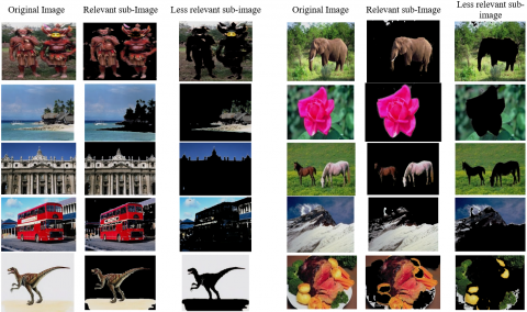
Figure 1 shows the framework for the active feature-based learning CBIR system. It consists of three stages i.e., pre-learning, training, and query processing. In the pre-learning stage, images of a class are transferred to the CIE L*a*b* color space. Each image is divided into four sub-images i.e., green, red, blue, and yellow using zero thresholding along the a* and b* axis as discussed in Algo-1.
The mean of the standard deviation of LBPNZ features for all the four-color spaces is calculated. The color space having minimum standard deviation implies the images are more stable through that color space for the class. The LBPNZ feature of this color space is selected as the more relevant texture feature or the active feature and the axis is considered the reference axis. The LBPNZ features of the sub-image in the reciprocate color space of the reference axis are selected as the less relevant texture feature. The more relevant texture feature is shown in italics-bold, and less relevant texture features are in only italics for each class in Table 2. The feature weights of both more and less relevant sub-images and reference axis information are stored, respectively. For each class, the value of, and are computed dynamically as mentioned in Alog-1.
|
Algo-1: Compute the reference axis and feature weights for each class:
|
Figure 1. Active feature-based learning framework for image retrieval
During the training, images are transferred to CIE L*a*b* color space. The LBPNZ features of more and less relevant sub-image are computed separately according to the pre-calculated value of the reference axis. The weighted LBPNZ features of both sub-images are fused together to build the final feature vector. The steps to build the feature database are mentioned in Algo-2. As the weights are calculated dynamically for each class, the fused feature vector represents the image with an enhanced signature of its belonging class.
|
Algo-2: Compute the active feature vector:
where, LBPki, Wki are LBP features and weights for relevant sub-image. LBPk’i, Wk’i are LBP features and weights for less relevant sub-image. |
|
Algo-3: Image query
|
In the case of query processing, first, the image is transferred to CIE L*a*b* color space. Then to compare the query image with the images of a class, the fused weighted feature vector is created using the reference axis and the weight values of that class. The distances of the query image feature and the database features of the class are computed. This process is replicated for all other classes. The top similar images are retrieved from the database according to their similarity measure. The detailed process is described in Algo-3.
The performance of the proposed active feature-based learning framework is analyzed using Minimum Distance Classifier (MDC) [13]. Average precision and recall analysis is done with different distance measures such as Euclidean, City Block, Canberra, and Extended Canberra distances [10]. The top 10 images are retrieved according to their similarity value in ascending order. Again, other standard classifiers such as Naïve Bayes and Support Vector Machine (SVM) [13] are also used to compare the performance of LBP and the proposed LBPCW feature vector.
3.6 Implementation of active feature selection
Figure 2 shows more and less relevant sub-image with their reference axis for each class. The b* is the reference axis for the People, Beach, Building, Bus, Dinosaur, Elephant, Glader, and Food classes. Yellow is the relevant color space for the Dinosaur class, and blue is the relevant color space for all the other classes. Whereas red is the relevant color space for both flower and horse classes along the a* axis.
The average standard deviation value of LBPNZ features are shown in Table 2 class-wise. The first column shows the mean values of the grayscale image, the mean values of green and red color sub-image along a* axis, and the blue and yellow color sub-images along b* axis are shown in the successive columns. The difference in the mean values of more and less relevant sub-images consequence disparity in their feature weights in the proposed CBIR framework.
Table 2. Class-wise mean variance of LBPNZ along CIE L*a* b*
|
a* axis |
b* axis |
||||
|
LBPGray |
LBPG |
LBPR |
LBPB |
LBPY |
|
|
People |
112.72 |
127.65 |
150.50 |
100.05 |
186.57 |
|
Beach |
137.20 |
255.89 |
208.09 |
94.19 |
162.37 |
|
Building |
146.65 |
179.44 |
169.94 |
98.23 |
141.17 |
|
Bus |
76.18 |
75.49 |
99.03 |
73.13 |
81.41 |
|
Dinosaur |
81.93 |
100.33 |
127.22 |
83.64 |
68.54 |
|
Elephant |
111.63 |
202.53 |
226.69 |
90.28 |
175.19 |
|
Flower |
126.25 |
119.03 |
104.81 |
118.56 |
170.29 |
|
Horse |
95.09 |
185.14 |
90.84 |
91.90 |
150.52 |
|
Gladder |
167.30 |
222.64 |
205.36 |
139.59 |
208.22 |
|
Food |
118.64 |
115.33 |
190.79 |
110.92 |
219.36 |
3.7 Distance measures
In the case of the minimum distance classifier, the distance measure plays an imperative role in finding the inter-class and intra-class distances [10]. The performance analysis of the LBPCW texture feature is shown in the result section. Figure 3 and Figure 4 illustrate the performance of the average retrieval rate using five different distance measures such as Euclidean (ED), City-block (CT), Chi-square (CHI), Canberra (CNB), and Extended-Canberra (ECNB) distances [10, 13]. Euclidean distance:
$D_{E D}=\sqrt{\sum_{i=0}^{L-1}\left(F_i^q-F_i^t\right)^2}$ (7)
City Block distance:
$D_{C T}=\sum_{i=0}^{L-1}\left|F_i^q-F_i^t\right|$ (8)
Canberra distance:
$D_{W T}=\sum_{i=0}^{L-1} \frac{\left|F_i^q-F_i^t\right|}{F_i^q+F_i^t}$ (9)
Chi-square:
$D_{C h i}=\sum_{i=0}^{L-1} \frac{\left(F_i^q-F_i^t\right)^2}{F_i^q+F_i^t}$ (10)
Extended Canberra distance:
$D_{E C D}=\sum_{i=0}^{L-1} \frac{\left|F_i^q-F_i^t\right|}{\left(F_i^q+\mu^q\right)+\left(F_i^t+\mu^t\right)}$, (11)
where
$\mu^q=\frac{1}{L} \sum_{i=0}^{L-1} F_i^q$ and $\mu^t=\frac{1}{L} \sum_{i=0}^{L-1} F_i^t$
3.8 Performance measures
The performance of the proposed CBIR framework is measured by the ratio of the number of correct predictions vs the total number of predictions. The average precision P (L) and average recall R(L) are computed as mentioned in Eq. (12) and Eq. (13) [8]. The average retrieval rate (ARR) represents the overall performance of a classifier [9]. A higher value of ARR implies more of the Area Under Curve (AUC) i.e., better performance. The precision vs recall curves for LBP and LBPCW feature vectors are shown in Figure 3.
The average precision
$P(L)=\frac{1}{N_t L} \sum_{q=1}^{N_t} n_q(L)$ (12)
The average recall
$R(L)=\frac{1}{N_t N_R} \sum_{q=1}^{N_t} n_q(L)$ (13)
where, L represents the retrieved image set
nq(L) denotes the number of correctly retrieved images due to the query image q;
Nt show the number of images in the database;
NR denote the number of relevant images in the database.
$A R R=\frac{1}{N_t N_R} \sum_{q=1}^{N_t} n_q\left(N_R\right)$ (14)
(a)
(b)
Figure 3. PR curve using LBP and LBPCW features
(a)
(b)
Figure 4. Class-wise retrieval
In this section, the performance of the proposed framework is reported with the help of extensive experimental results. The PR curve of the LBP and the proposed LBPCW feature of Wang-1K dataset images using MDC with five distance measures namely Euclidean, City-block, Chi-square, and Canberra and Extended-Canberra distance are presented in Figure 3. Figure 3(a) shows the average precision vs average recall curve (PR curve) using LBP and Figure 3(b) represents the PR curve using our proposed LBPCW feature. These figures clearly indicate the supremacy of the LBPCW feature over the standard LBP feature in terms of average precision and recall. It is worth mentioning here that the ECNB distance measure gives better results for the LBP feature, whereas the City-Block distance measure performs better for the LBPCW feature. We have presented the performance of the individual classes using the five distance measures in Figure 4(a) and 4(b) for LBP and LBPCW respectively. These figures illustrate the enhancement of the performance in all classes except the bus class using the LBPCW feature. It is worth mentioning that the performance of the classes having complex backgrounds such as People, beach, and Elephant is enhanced using the LBPCW feature. The overall performance of LBPCW is better than LBP due to feature space discrimination.
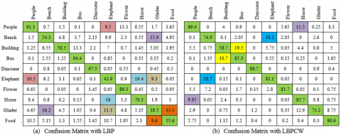
Table 3 shows the top 10 retrieval values using MDC for the LBP and LBPCW features of Wang-1K images. The performance of LBPCW is better for all the classes except bus class. Since the bus class is having different color buses, the feature weight value is biased and that affects the performance of bus class. However, the overall performance of LBPCW improved significantly. Figure 5(a) presents the confusion matrix for LBP, and Figure 5(b) shows the confusion matrix for LBPCW with CT block distance measure. Figure 5(a) indicates that intervention of Elephant class with People, Horse and Glader classes are high. Similarly, there is lot of overlapping of the Glader class with Beach and food classes. It indicates that the images with similar background are having more interference. On the other hand the Figure 5(b) shows there exist interference between the People with Horse, Beach with Elephant, and Building with Bus, which is comparitively less.
Figure 6(a) shows a comparative analysis of two best-performing PR curves for both texture features. First the LBP with Canberra and Extended Canberra distances, second the LBPCW with City-block and Extended Canberra distances, which indicates the performance of LBPCW with City-block outperforms than the others.
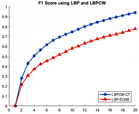
The F1 score presents the harmonic mean of the average precision vs average recall value [29]. It is used to ascertain the bias of the feature vectors for a class by analyzing the results of a classifier.
The F1 score is calculated as:
$F 1 \_$Score $=2 \times \frac{\text { Average precision } \times \text { Average recall }}{\text { Average precision }+ \text { Average recall }}$ (15)
Figure 6(b) presents the F1 score of LBP and LBPCW, it is worth of mentioning the harmonic mean of LBPCW is better with respect to the LBP for top 20 retrieved images of Wang 1K dataset.
Table 3. Shows the top 10 retrieval using MDC
|
(a) Images retrieved using LBP |
(b) Images retrieved using LBPCW |
|||||||||
|
ED |
CT |
CNB |
CHI |
ECNB |
ED |
CT |
CNB |
CHI |
ECNB |
|
|
People |
63.30 |
67.60 |
64.90 |
66.90 |
68.80 |
71.80 |
75.60 |
70.00 |
75.70 |
76.60 |
|
Beach |
46.60 |
57.20 |
58.30 |
58.90 |
62.20 |
74.00 |
74.80 |
72.10 |
75.60 |
73.20 |
|
Building |
44.90 |
59.40 |
65.70 |
59.00 |
67.70 |
63.50 |
69.70 |
71.00 |
67.10 |
71.10 |
|
Bus |
88.20 |
95.30 |
95.10 |
95.90 |
96.00 |
76.40 |
81.90 |
77.30 |
81.20 |
79.70 |
|
Dinosaur |
96.40 |
97.70 |
96.70 |
98.20 |
97.70 |
98.70 |
98.90 |
93.90 |
99.00 |
98.30 |
|
Elephant |
41.10 |
50.10 |
55.40 |
51.00 |
55.70 |
86.10 |
86.50 |
86.00 |
86.90 |
85.50 |
|
Flower |
82.10 |
88.30 |
90.00 |
88.80 |
90.90 |
76.00 |
89.10 |
86.10 |
39.10 |
92.50 |
|
Horse |
77.00 |
81.10 |
82.10 |
81.30 |
81.50 |
88.30 |
89.30 |
90.20 |
89.60 |
89.40 |
|
Glader |
36.40 |
38.50 |
38.10 |
40.50 |
40.10 |
83.10 |
81.10 |
61.00 |
85.60 |
75.20 |
|
Food |
47.50 |
58.60 |
63.60 |
60.30 |
63.80 |
86.30 |
93.90 |
86.00 |
93.70 |
84.80 |
Figure 5. Confusion matrix using LBP and LBPCW
|
Figure 6(a). PR curve of LBP and LBPCW with two best distances |
Figure 6(b). Shows F1 score LBP vs LBPCW with their best distance |
Table 4. Classification performance for Wang-1K using Naive Bayes and SVM
|
Naïve Bayes |
SVM |
|||||
|
LBP |
LBPSM |
LBPCW |
LBP |
LBPSM |
LBPCW |
|
|
People |
51.33 |
70.34 |
87.38 |
68.87 |
82.41 |
97.94 |
|
Beach |
61.26 |
64.04 |
82.08 |
72.82 |
81.19 |
97.96 |
|
Building |
73.20 |
72.83 |
97.83 |
82.35 |
89.29 |
97.09 |
|
Bus |
71.28 |
85.84 |
98.02 |
93.48 |
88.89 |
99.00 |
|
Dinosaur |
87.50 |
92.16 |
91.59 |
98.96 |
99.00 |
97.85 |
|
Elephant |
38.21 |
64.22 |
89.69 |
72.90 |
82.30 |
97.06 |
|
Flower |
78.63 |
90.72 |
96.04 |
92.16 |
96.70 |
99.01 |
|
Horse |
60.83 |
82.24 |
92.52 |
73.87 |
91.26 |
97.09 |
|
Glader |
62.79 |
73.91 |
85.86 |
74.51 |
97.85 |
98.99 |
|
Food |
71.59 |
79.73 |
96.81 |
74.76 |
88.89 |
98.99 |
|
Average Retrieval |
65.00 |
77.37 |
91.22 |
81.10 |
89.88 |
98.00 |
Table 4 shows the class-wise retrieval of the images for the Wang-1K dataset with the LPB, local binary pattern with saliency map (LBPSM) [14] and the LBPCW feature vectors using the Naïve Bayes and SVM with linear kernel classifiers. The retrieval rate is enhanced in case of LBPCW feature for both the classifiers. Again, the performance of the SVM is better than the Naïve Bayes due to its optimal margin selection. The LBPSM feature outperforms for the Dinosaur class. The average retrieval rate of the SVM with LBPSM is 89.88% and 98.00% using LBPCW.
The Corel-5K database images are tested with the proposed active feature-based learning framework, the performance of the different classifiers is reported in Table 5 It shows the average retrieval rate of the SVM using LBPSM is 85.46% and with LBPCW is 95.35%. The performance of the LBP feature is better for the dog class in comparison to the other two features. Possibly the result of the dog class is biased due to variant color dogs in the Corel-5K dataset.
Table 5. Classification performance for Corel 5K using Naive Bayes and SVM
|
Naïve Bayes |
SVM |
|||||
|
LBP |
LBPSM |
LBPCW |
LBP |
LBPSM |
LBPCW |
|
|
Lion |
46.11 |
59.41 |
55.88 |
61.82 |
88.78 |
92.78 |
|
Iceberg |
52.27 |
70.00 |
71.82 |
71.43 |
86.14 |
94.95 |
|
Pyramid |
60.91 |
80.99 |
91.75 |
77.19 |
87.88 |
97.06 |
|
Dog |
88.98 |
73.47 |
85.45 |
98.95 |
80.81 |
98.02 |
|
Monument |
43.07 |
71.07 |
87.27 |
74.38 |
75.93 |
96.12 |
|
Beach |
48.98 |
56.20 |
72.82 |
62.50 |
87.23 |
87.85 |
|
Stone |
85.15 |
62.86 |
91.59 |
85.19 |
80.00 |
98.99 |
|
Car |
76.14 |
82.05 |
89.77 |
87.80 |
87.00 |
96.94 |
|
Dinosaur |
70.00 |
83.87 |
92.78 |
71.60 |
86.00 |
95.88 |
|
Fish |
72.04 |
70.65 |
91.23 |
88.16 |
94.79 |
94.90 |
|
Average Retrieval |
64.37 |
71.06 |
83.04 |
77.90 |
85.46 |
95.35 |
In this paper, we have proposed an active feature-based learning framework in the CIE L*a*b* color space. This color space is highly correlated with human perception. Using the visual property of a class each image is divided into two sub-images i.e., more and less relevant sub-images. These sub-images are produced by analyzing the mean of the standard deviation of their LBP feature class-wise. As these sub-images contain many zero-valued pixels, we have proposed an LBPNZ feature-finding technique that considers only the non-zero pixels for calculating the LBP. In the case of class-wise performance analysis using LBP feature, the retrieval rate of the Bus and Dinosaur classes are better. It is interesting to observe that the mean values of the more and less relevant sub-images are highly correlated in these two classes. To provide high priority to the more relevant sub-image, the weighted feature fusion technique is used. The performance proposed framework is tested with two public datasets i.e., Wang-1K and Corel-5K. The result analysis shows the SVM with LBPCW features outperforms in comparison to MDC, Naïve Bayes classifier. In addition to the retrieval rate PR curve and F1 score measures are presented in the result section. The average retrieval rate using our proposed LBPCW model is 91.22% using the Naïve Bayes classifier and 98.00% with SVM for Wang-1K dataset. The average retrieval is 83.04% and 95.35% using Naïve Bayes and SVM classifiers respectively for the Corel-5K dataset. Moreover, the retrieval rate of the image classes having complex backgrounds such as the Elephant, People, and Horse are improved using the proposed LBPCW. Further analysis can be done in the CIE L*a*b* color space for computing ROI effectively. As a part of the future scope, more robust image ranking can be explored using the adaptive feature weights for saliency image segments, which happens partially with the proper batch selection in CNN.
[1] Feng, S., Xu, D., Yang, X. (2010). Attention-driven salient edge (s) and region (s) extraction with application to CBIR. Signal Processing, 90(1): 1-15. https://doi.org/10.1016/j.sigpro.2009.05.017
[2] Alzu’bi, A., Amira, A., Ramzan, N. (2015). Semantic content-based image retrieval: A comprehensive study. Journal of Visual Communication and Image Representation, 32: 20-54. https://doi.org/10.1016/j.jvcir.2015.07.012
[3] Sharif, U., Mehmood, Z., Mahmood, T., Javid, M.A., Rehman, A., Saba, T. (2019). Scene analysis and search using local features and support vector machine for effective content-based image retrieval. Artificial Intelligence Review, 52: 901-925. https://doi.org/10.1007/s10462-018-9636-0
[4] Hamreras, S., Boucheham, B., Molina-Cabello, M.A., Benitez-Rochel, R., Lopez-Rubio, E. (2020). Content based image retrieval by ensembles of deep learning object classifiers. Integrated Computer-aided Engineering, 27(3): 317-331. https://doi.org/10.3233/ICA-200625
[5] Dubey, S.R. (2021). A decade survey of content based image retrieval using deep learning. IEEE Transactions on Circuits and Systems for Video Technology, 32(5): 2687-2704. https://doi.org/10.1109/TCSVT.2021.3080920
[6] Unar, S., Wang, X., Wang, C., Wang, Y. (2019). A decisive content based image retrieval approach for feature fusion in visual and textual images. Knowledge-Based Systems, 179: 8-20. https://doi.org/10.1016/j.knosys.2019.05.001
[7] Jena, P.K., Khuntia, B., Anand, R., Patnaik, S., Palai, C. (2020). Significance of texture feature in NIR face recognition. In 2020 First International Conference on Power, Control and Computing Technologies (ICPC2T), IEEE, pp. 21-26. https://doi.org/10.1109/ICPC2T48082.2020.9071504
[8] Xia, Z., Jiang, L., Liu, D., Lu, L., Jeon, B. (2019). BOEW: A content-based image retrieval scheme using bag-of-encrypted-words in cloud computing. IEEE Transactions on Services Computing, 15(1): 202-214. https://doi.org/10.1109/TSC.2019.2927215
[9] Celik, C., Bilge, H.S. (2017). Content based image retrieval with sparse representations and local feature descriptors: a comparative study. Pattern Recognition, 68: 1-13. https://doi.org/10.1016/j.patcog.2017.03.006
[10] Srivastava, P., Khare, A. (2017). Integration of wavelet transform, local binary patterns and moments for content-based image retrieval. Journal of Visual Communication and Image Representation, 42: 78-103. https://doi.org/10.1016/j.jvcir.2016.11.008
[11] Singh, C., Walia, E., Kaur, K.P. (2018). Color texture description with novel local binary patterns for effective image retrieval. Pattern Recognition, 76: 50-68. https://doi.org/10.1016/j.patcog.2017.10.021
[12] Garg, M., Dhiman, G. (2021). A novel content-based image retrieval approach for classification using GLCM features and texture fused LBP variants. Neural Computing and Applications, 33: 1311-1328. https://doi.org/10.1007/s00521-020-05017-z
[13] Tiwari, A.K., Kanhangad, V., Pachori, R.B. (2017). Histogram refinement for texture descriptor based image retrieval. Signal Processing: Image Communication, 53: 73-85. https://doi.org/10.1016/j.image.2017.01.010
[14] Pradhan, J., Kumar, S., Pal, A.K., Banka, H. (2018). A hierarchical CBIR framework using adaptive tetrolet transform and novel histograms from color and shape features. Digital Signal Processing, 82: 258-281. https://doi.org/10.1016/j.dsp.2018.07.016
[15] Singh, C., Walia, E., Kaur, K.P. (2018). Enhancing color image retrieval performance with feature fusion and non-linear support vector machine classifier. Optik, 158: 127-141. https://doi.org/10.1016/j.ijleo.2017.11.202
[16] Nazir, A., Ashraf, R., Hamdani, T., Ali, N. (2018). Content based image retrieval system by using HSV color histogram, discrete wavelet transform and edge histogram descriptor. In 2018 International Conference on Computing, Mathematics and Engineering Technologies (iCoMET), IEEE, pp. 1-6. https://doi.org/10.1109/ICOMET.2018.8346343
[17] Alsmadi, M.K. (2020). Content-based image retrieval using color, shape and texture descriptors and features. Arabian Journal for Science and Engineering, 45(4): 3317-3330. https://doi.org/10.1007/s13369-020-04384-y
[18] Liu, P., Guo, J.M., Chamnongthai, K., Prasetyo, H. (2017). Fusion of color histogram and LBP-based features for texture image retrieval and classification. Information Sciences, 390: 95-111. https://doi.org/10.1016/j.ins.2017.01.025
[19] Verma, M., Raman, B., Murala, S. (2015). Local extrema co-occurrence pattern for color and texture image retrieval. Neurocomputing, 165: 255-269. https://doi.org/10.1016/j.neucom.2015.03.015
[20] Mistry, Y., Ingole, D.T., Ingole, M.D. (2018). Content based image retrieval using hybrid features and various distance metric. Journal of Electrical Systems and Information Technology, 5(3): 874-888. https://doi.org/10.1016/j.jesit.2016.12.009
[21] Ahmed, K.T., Ummesafi, S., Iqbal, A. (2019). Content based image retrieval using image features information fusion. Information Fusion, 51: 76-99. https://doi.org/10.1016/j.inffus.2018.11.004
[22] Bai, C., Chen, J.N., Huang, L., Kpalma, K., Chen, S. (2018). Saliency-based multi-feature modeling for semantic image retrieval. Journal of Visual Communication and Image Representation, 50: 199-204. https://doi.org/10.1016/j.jvcir.2017.11.021
[23] Zhang, J., Feng, S., Li, D., Gao, Y., Chen, Z., Yuan, Y. (2017). Image retrieval using the extended salient region. Information Sciences, 399: 154-182. https://doi.org/10.1016/j.ins.2017.03.005
[24] Ahsani, A.F., Sari, Y.A., Adikara, P.P. (2019). Food image retrieval with gray level co-occurrence matrix texture feature and CIE L* a* b* color moments feature. In 2019 International Conference on Sustainable Information Engineering and Technology (SIET), IEEE, pp. 130-134. https://doi.org/10.1109/SIET48054.2019.8985990
[25] Krishnamoorthy, R., Devi, S.S. (2013). Image retrieval using edge based shape similarity with multiresolution enhanced orthogonal polynomials model. Digital Signal Processing, 23(2): 555-568. https://doi.org/10.1016/j.dsp.2012.09.018
[26] Reta, C., Cantoral-Ceballos, J.A., Solis-Moreno, I., Gonzalez, J.A., Alvarez-Vargas, R., Delgadillo-Checa, N. (2018). Color uniformity descriptor: An efficient contextual color representation for image indexing and retrieval. Journal of Visual Communication and Image Representation, 54: 39-50. https://doi.org/10.1016/j.jvcir.2018.04.009
[27] Palai, C., Pattanaik, S.R., Jena, P.K. (2020). Significance of the background image texture in cbir system. In Computational Intelligence in Data Mining: Proceedings of the International Conference on ICCIDM, Springer Singapore, pp. 489-500. https://doi.org/10.1007/978-981-13-8676-3_42
[28] Aziz, M.A.E., Ewees, A.A., Hassanien, A.E. (2018). Multi-objective whale optimization algorithm for content-based image retrieval. Multimedia Tools and Applications, 77: 26135-26172. https://doi.org/10.1007/s11042-018-5840-9
[29] Satpathy, A., Jiang, X., Eng, H.L. (2014). LBP-based edge-texture features for object recognition. IEEE Transactions on Image Processing, 23(5): 1953-1964. https://doi.org/10.1109/TIP.2014.2310123
[30] Liu, G.H., Yang, J.Y. (2013). Content-based image retrieval using color difference histogram. Pattern Recognition, 46(1): 188-198. https://doi.org/10.1016/j.patcog.2012.06.001