Chetan R* | D.V. Ashoka | Ajay Prakash B V
© 2022 IIETA. This article is published by IIETA and is licensed under the CC BY 4.0 license (http://creativecommons.org/licenses/by/4.0/).
OPEN ACCESS
Agriculture is the main occupation of rural India, which promotes economic growth in the country's development. To increase the yield of the crops to feed the increasing population, it is essential to identify the crops which can be grown in the respective zones. In this article, the Fused Classifier Algorithm (FCA) and Interfused Machine Learning Algorithm (IMLA) are proposed to predict crops suitable for the land based on the zones and agro-climatic parameters. Focusing on the zones of the Karnataka region, the model predicts the crop to the farmers. The different machine learning models such as naïve Bayes, decision tree, neighbors, multilayer perceptron have also been evaluated by varying the hyperparameters and checked for accuracy of the models built. The FCA algorithm merges different algorithms using the error rate with hyperparameters tuning and is given to IMLA to predict crops. This article also compares different machine learning classifiers with the proposed IMLA algorithm, which shows better accuracy with 82.7%.
machine learning, ensemble learning, agro-ecological zones, crop prediction, big data
The main source of income for the majority of rural people in India is agriculture. Due to the increase in population, the yield of crops is not sufficient. Even though India is one of the biggest producers of agricultural products, it has less farm productivity. The most Indian farmers rely on their intuition to decide which crop to plant in a particular season. They find comfort following the agricultural patterns and norms of their ancestors. Unaware of the fact that crop production is situationally and highly dependent on current climate and soil conditions.
The economic growth is promoted by agriculture and also a path to development of rural areas. The use of improved technology in agricultural practices is less common in India. Due to such ancient practice, the crop yield has not been measured by the farmer, and he has lost hope for the agricultural process. Many farmers who neglected to farm also set up other professions. Sometimes, farmers' suicide also increased.
Thus, there is a necessity for technical support in the field of agriculture. Agriculture is done from ages, the data from the past is collected furthermore used for the suggestion of crops. This work will help farmers to choose a proper crop for the land based on agro-ecological zones (AEZ). The suggestions are made using the agro-ecological zones plus climatic parameters, soil parameters, and temperature.
This article proposes two algorithms fused classifier algorithm and interfused machine learning algorithm for crop prediction. The main contribution of this work is:
The article describes the related work, machine learning classifiers, the proposed algorithms.
This section is going to describe the existing methods that are available for crop recommendation and prediction; it also describes different machine learning algorithms used as well as the accuracy of the models.
The crop suggestion model [1] uses a random forest algorithm for crop suggestion with 80 percent accuracy and fertilizer selection which uses an apriori algorithm. An android app is developed that can be used by the farmers for crop suggestions. This model uses only climatic parameters and fertilizers for crop suggestions. The limitations here is the soil parameters also play a vital role in crop suggestion which is not considered. A recommendation model [2] uses the weblog data for learning the user profiles and recommends the articles based on the demands and online behaviors. A recommendation system [3] for crops based on association rule mining and generic algorithm is a very complex system since it uses a genetic algorithm, and time complexity will be more for the prediction of crops. The model is complex and time taken to recommend will be more.
The fuzzy model [4] for the recommendation of crops is going to suggest crops to farmers based on the weather condition and location information. IoT model [5] uses random forest and naïve bayes algorithm for crops prediction using sensor data by considering values such as temperature, moisture also ph of soil data. The model does not use the environment data since it is also required for crop suggestion. A hybrid decision support system [6] was used for the prediction of crop yield. This system used the ANN data mining technique for the prediction of yield.
An architecture that uses big data analysis for agricultural intelligent decision systems [7] studied the wheat production using the decision system. It decides plant variety selection, decision for time of sowing seeds, decision for frost period, green stage, amount of planting, and decision for fertilization. Decision support system [8] was build using the web framework for cassava cultivation using soil data, and for data pre-processing weka tool was used using arff convertor. A framework for recommending the crops for farmers [9] detects the user's location, and based on agro-climatic data, it generates the similarity index and selects the top 10 similarities for recommending the crops. A decision system is build using data mining algorithms [10] for farmers to select crops for cultivation mapping using different parameters like soil ph value, soil type, weather, water required, and temperature range.
A framework for monitoring the agriculture yield using distributed computing with customized cloud servers [11]. A comprehensive review on applications of machine learning in agriculture and different machine learning algorithms [12] used for crop prediction, yield prediction, and other works. It gives a research gap in the crop prediction using machine learning. From the existing works, the authors find out still an improved crop suggestion and prediction model required for the suggestion of crops based on the agro-ecological zones.
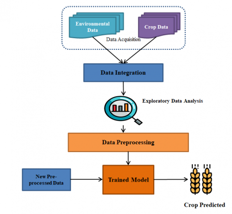
Figure 1. Proposed Methodology for prediction of crops based on AEZ
The proposed methodology for predicting the crops in the agro-ecological zone (AEZ) is based on the agricultural data and weather data by building different machine learning models using classifiers. Figure 1 shows the proposed methodology for the prediction of crops based on AEZ. The proposed methodology, divided into i) data acquisition ii) data integration iii) exploratory data analysis iv) data pre-processing v) building machine learning models vi) prediction of crops based on AEZ. In the next sections, the above steps are discussed.
3.1 Data acquisition
For predicting the crops, first data acquisition plays an important role. There are ten agro-ecological zones in Karnataka, and crops are going to vary from zone to zone depending upon the rainfall, temperature, and season. So important parameters required for crop prediction are area of land cultivated, agro-ecological zones, production of crop, rainfall, precipitation, and temperature. The data was collected for crops like rice, ragi, groundnut, and sunflower of 30 districts of Karnataka from the government of India website [13].
3.2 Data integration
In this step, data is integrated from different sources, such as agro-climatic data and crop production in various districts. The agricultural district-wise crop data collected consists of area, production, and yield of crops year-wise from central government [13] and Karnataka government websites [14]. Rainfall of different district year wise was collected from Karnataka statistical website [15]. Precipitation, temperature, and humidity data were collected from a weather monitoring website [16]. The collected data from different sources has to be integrated into a single dataset for the prediction of crops.
3.3 Exploratory data analysis
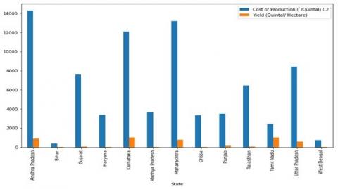
EDA is performed to analyze a dataset, from which visualization techniques were used to summarize the key characteristics of the data. EDA is primarily used to see what data tells us beyond formal modeling. It also helps us in extracting the important variables; it provides deep insight into the data and uncovers the underlying structures. Figure 2 shows the comparison of the cost of production and the yield produced from the government statistics. It shows that yield produced is less even though the cost involved in production is more this is mainly due to the selection of crops which are not suitable for the land and dependent on soil and environment parameters and also major effect would be rainfall.
Figure 2. Cost of production and yield state-wise
3.4 Data pre-processing
3.4.1 Handling missing values
The dataset contains numeric values average of features or columns is calculated and replaced by missing values with the calculated average.
3.4.2 Handling categorical values
Categorical data refers to information that has specific categories in our dataset like district, AEZ, and crop names. The categorical values are converted into numerical values since the machine learning models understand only numerical values.
3.4.3 Normalization
Normalization of the attributes is done to reduce the scales and improve the model performance. The min-max normalization technique was used for normalizing the data. The equation given below shows the min-max normalization.
$\mathbf{x}^{\mathbf{1}}=\frac{\mathrm{x} \text {-average }(\mathrm{x})}{\max (\mathrm{x})-\min (\mathrm{x})}$ (1)
3.4.4 Splitting data into train/test
The dataset is split into train/test data and given into machine learning models for getting trained and tested. The train data is the subset of the dataset used for training the machine learning model. Test dataset is another subset of the dataset used for testing the model to predict the outcomes. The dataset was split into 80:20 ratios, where 80 percent were taken for training the model and 20 percent used for testing the model. The dataset was also split into 70:30, and a model comparison is made.
4.1 Naïve Bayes classifier
The Naive Bayes classifier is a machine learning probabilistic model used for classification tasks. The classifier is based on the Bayesian theorem explained in Ref. [17]. Select the dataset and train the model. When the crop is suitable for the zone due to its characteristics, suggest it for cultivation. The columns represent the characteristics, and the rows represent the inputs. Bayes' theorem can be written as in Eq. (2):
$\mathbf{P}(\mathbf{a} \mid \mathbf{B})=\frac{\mathbf{P}(\mathbf{B} \mid \mathbf{a}) \mathbf{P}(\mathbf{a})}{\mathbf{P}(\mathbf{B})}$ (2)
The variable a is the target class (Crop). Variable B represents the parameters/features; they can be mapped to aez_zone, rainfall, area, production, precipitation, humidity, max_temperature, min_temperature, and mean_temperature.
4.2 Decision tree classifier
A decision tree classifier is a classification method most used widely. It uses a tree for making decisions to go from observations about a feature to finish about the target leaf value. The detailed model of the target variable can take a distinct set of values called classification trees. For the classifier the target variable y is the crop to be classified and dependent variables are (x1, x2... xn) which are soil and climate data. The gini index is calculated and attribute with less gini index is preferred for generating the tree. The gini index is calculated using the Eq. (3).
Gini index $=1-\sum_{j j} 2$ (3)
4.3 Neural network classifier
Multilayer perceptron (MLP) is a type of artificial progressive neural network (ANN). The term MLP is sometimes flexible for forwarding ANNs and sometimes strictly to refer to networks that consist of multiple layers of perceptrons.
Three layers of MLP are the input layer, output layer, and hidden layer. A non-linear activation function is used by a neuron which is the node that expects the input nodes. For training, MLP backpropagation which is a supervised learning technique, is used. Its multiple layers and non-linear activation distinguish linear from multi-linear perceptrons.
4.4 K-neighbors classifier
K-nearest neighbors classifier is one of the simplest and a non-parameter-based slow algorithm in machine learning. Non-parametric means one that does not make any assumptions about the underlying data. That is, the choice is based on the approximate values to other data points, nevertheless of the characteristic that the number represents. A slow learning algorithm means no training phases or few present. Thus, new data points will be categorized as soon as they appear.
4.5 Random forest classifier
Random forest classifier is a supervised learning algorithm that is used for regression as well as classification problems. A forest is made up of trees, and the more trees there, the more robust the forest is. Random Forest builds a decision tree on a randomly selected sample of data and gets its prediction. It also provides a very good indicator of the importance of each tree's characteristics and votes to select the best solution.
4.6 XGBoost classifier
XGBoost is an ensemble learning method used for supervised learning problems. The prediction is given as a linear union of input parameters with weights.
$\mathbf{y}_{\mathbf{i}}=\sum_{\mathbf{j}} \boldsymbol{\theta}_{\mathbf{j}} \mathbf{x}_{\mathbf{i j}}$ (4)
The predicted value varies based on the job. The job of model training is the same as figuring out optimal features that best fit. For model training, an objective function is defined to measure how the training model fits. The function consists of training loss as well as regularization, as shown below.
$\mathbf{0 b j}(\boldsymbol{\theta})=\mathbf{l}(\boldsymbol{\theta})+\Omega(\boldsymbol{\Theta})$ (5)
In Eq. (5), where l is the loss function for training and omega is a term used for regularization. L is chosen as the mean squared error. The complexity of the model is controlled by the regularization term, which avoids overfitting. The model is trained with additional parameters like the number of estimators, learning rate, maximum features, and maximum tree depth.
In the proposed methodology, two algorithms fusing classifier algorithm (FCA) and interfused ensemble learning algorithm (IELA), have been proposed for the prediction of crops. The fusing classifier algorithm takes the training data Xtrain and Ytrain as the input. It outputs the fused classifier model, which is the combination of different machine learning models discussed above. First, the input features x1, x2… xn are selected, and null values are removed by replacing them with mean values of xi. Then min-max normalization operation is performed to normalize the training data. The min-max normalization is performed due to reduce the authenticity of the data when replacing the null values by average and to make sure the data is reliable. The null values present are very less and that to in the variables like production, area and yield which are of less important. The hyper parameters hpi for different machine learning models are initialized and tuned for reducing the error rate E. If the models error rate Ei is less than the MINthreshold, then that model is added for fusing. Otherwise, the hyperparameters are tuned once again until the error rate is less than MINthreshold.
---------------------------------------------------------------------
Algorithm 1: Fusing Classifier Algorithm
----------------------------------------------------------------------
Input: Training Data {Xtrain, Ytrain}
Output: Fused Classifier Model [FCM]
----------------------------------------------------------------------
The returned FCM model is used as input in the Interfused Machine Learning (IML) algorithm described below. The IML algorithm reads the new data where it has to predict the crop based on the features given as input. The IML algorithm uses the loss function MSE for individual features as well as entire data by choosing the activation function σ is used for predicting the target class. The gradient cost function is used as the optimization function for getting the better results.
-----------------------------------------------------------------------
Algorithm 2: Interfused Machine Learning Algorithm
-----------------------------------------------------------------------
Input: Test data Xtest, Fused Classifier Model (FCM)
Output: predict labels y^test
1. for each xido
2. $\mathrm{x} . \mathrm{w}=\sum_{i=0}^{n}\left(x_{i} * w_{i}\right)$
3. Q = x.w + b
4. for each yido
5. calculate loss function $\mathrm{MSE}_{\mathrm{i}}=\left(y_{i}-\widehat{y}_{l}\right)^{2}$
6. compute loss function for entire data $\mathrm{C}=\frac{1}{n} \sum_{i=1}^{n}\left(y_{i}-\widehat{y}_{l}\right)^{2}$
7. for each wi do
8. compute the gradient cost function $\frac{\partial \mathrm{C}}{\partial \mathrm{w}_{\mathrm{i}}}=\frac{\partial \mathrm{C}}{\partial \widehat{\mathrm{y}}} * \frac{\partial \widehat{\mathrm{y}}}{\partial \mathrm{z}} * \frac{\partial \mathrm{z}}{\partial \mathrm{w}_{\mathrm{i}}}$
9. $\frac{\partial \mathrm{C}}{\partial \hat{\mathrm{y}}}=\frac{2}{\mathrm{n}} * \operatorname{Sum}(\mathrm{y}-\hat{\mathrm{y}})$
10. $\frac{\partial \hat{y}}{\partial z}=\sigma(Q) *(1-\sigma(Q))$
11. $\frac{\partial z}{\partial w_{i}}=x_{i}$
12. end for
13. end for
14. $\hat{y}=\sigma(\mathbf{Q})=\frac{1}{1+\mathrm{e}^{-\mathrm{q}}}$
15. return predict labels $\hat{y}$
-----------------------------------------------------------------------
The proposed methodology, implemented using Jupiter notebook with python programming language. Th e closest k neighboring features are learned using k-neighbors classifier model, where k is a user-specified integer value. For building our model from many runs, the model gave a good accuracy for a value of k=7. In KNN model minkowski distance measure [18] was used which will measure right angle distance principle, based on this principle we started varying k value from 1 to 7. We obtain better accuracy with the help of 7 nearby point by obtaining maximum similarity. For implementing MLP number of hidden layers used in the model is 5, and the activation function which is being used in building the model is rectified linear unit (ReLU). The ReLU activation function sets the negative value to zero and retains the value if it is a positive value. The Adam optimization technique is used for model training. Table 1 shows the results of evaluation metrics such as precision, recall, f1-score, and support of different ml models fused.
Table 1. Results of evaluation metrics such as precision, f1-score, recall, and support obtained from ML models
|
ML Model |
precision |
recall |
f1-score |
Support |
accuracy |
|
Naive Bayes |
0.60 |
0.57 |
0.55 |
296 |
57.43 |
|
Decision Tree |
0.72 |
0.72 |
0.72 |
296 |
71.95 |
|
MLP |
0.75 |
0.75 |
0.75 |
296 |
75 |
|
Kneighbors |
0.70 |
0.70 |
0.70 |
296 |
70.27 |
|
Random Forest |
0.83 |
0.83 |
0.83 |
296 |
82.77 |
|
Proposed (IML) Approach |
0.84 |
0.84 |
0.84 |
296 |
84.12 |
This section describes the predicted results of the crop recommended for the AEZ. The proposed methodology shown in Figure 1 is evaluated with different ml models by fusing them using the FCM algorithm using different hyperparameters, as discussed in the implementation section. The fused classifiers were naïve bayes, decision tree, kneighbors, neural network, random forest, and xgboost classifiers. In order to evaluate the proposed methodology following experimental setup has been considered. The train and test data were split for 80:20 and 70:30 for comparing the built ml models. For the decision tree model, parameter min_sample_split was used as 2 for splitting the tree. For the KNN model number of neighbors was set to 7. For MLP model activation function used was ReLU, and the optimization function used was Adam. For XGBOOST model, learning rate and estimators were varied to study the model, and the result obtained is shown in Table 2.
Table 2. Training score (TRN) and validation score (VLD) accuracy of the XGBoost model measured by varying the learning rate and estimators
|
Estimators |
10 |
20 |
30 |
60 |
80 |
90 |
100 |
|||||||
|
Learning rate |
TRN |
VLD |
TRN |
VLD |
TRN |
VLD |
TRN |
VLD |
TRN |
VLD |
TRN |
VLD |
TRN |
VLD |
|
0.05 |
74.8 |
69.9 |
76 |
71.6 |
79.1 |
73.3 |
82.1 |
74 |
85.9 |
74.3 |
86.8 |
76.4 |
87.6 |
77.4 |
|
0.1 |
75.8 |
69.3 |
79.2 |
73.3 |
85.8 |
75 |
90.9 |
77.7 |
92.8 |
78.7 |
93.4 |
79.1 |
95 |
79.7 |
|
0.25 |
80.7 |
71.6 |
87.8 |
75.7 |
94.9 |
78 |
97.5 |
79.4 |
99 |
78.7 |
99.7 |
79.4 |
99.9 |
79.7 |
|
0.5 |
86.6 |
75 |
94.1 |
79.7 |
99.2 |
80.7 |
99.9 |
82.1 |
99.9 |
83.1 |
100 |
82.8 |
100 |
82.4 |
|
0.75 |
90.2 |
73.6 |
97.6 |
76.7 |
100 |
79.4 |
100 |
79.7 |
100 |
79.4 |
100 |
80.1 |
100 |
79.1 |
|
1.0 |
92.3 |
78.7 |
97.6 |
80.4 |
100 |
81.1 |
100 |
81.4 |
100 |
82.8 |
100 |
83.4 |
100 |
84.1 |
Table 3. The results of evaluation metrics such as precision, recall, and f1-score obtained for all ML models for 80/20 and 70/30 train test ratio
|
ML Model |
NB |
DT |
MLP |
KNN |
RF |
Interfused |
||||||
|
Splitting ratio |
80/20 |
70/30 |
80/20 |
70/30 |
80/20 |
70/30 |
80/20 |
70/30 |
80/20 |
70/30 |
80/20 |
70/30 |
|
precision |
0.60 |
0.61 |
0.72 |
0.72 |
0.75 |
0.71 |
0.70 |
0.69 |
0.83 |
0.81 |
0.84 |
0.80 |
|
recall |
0.57 |
0.59 |
0.72 |
0.71 |
0.75 |
0.70 |
0.70 |
0.70 |
0.83 |
0.81 |
0.84 |
0.80 |
|
f1-score |
0.55 |
0.56 |
0.72 |
0.71 |
0.75 |
0.70 |
0.70 |
0.69 |
0.83 |
0.81 |
0.84 |
0.80 |
The models performances are evaluated using metrics such as accuracy, precision, recall, and F1 score has been used. Table 3 shows the comparison of performance metrics for different machine learning algorithms with proposed Interfused model. Accuracy is the ratio of observations predicted correctly to overall observations. Precision is the ratio of the sum of correctly predicted positive observations and observations that are positively predicted. Recall is the ratio of positive observations correctly predicted to all observations. F1 score is the average of recall and precision.
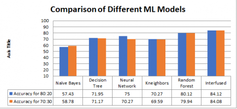
Figure 3. The accuracy achieved by ML models and interfused model
Figure 3 shows the accuracy achieved by different machine learning models. The interfused algorithm, along with random forest, has given a very good accuracy of above 80% in predicting the crops. The interfused approach used the error rate as the threshold for fusing the different models. The models with minthreshold error rate were fused together resulting in 84.12% accuracy which is comparatively better than random forest classifier.
The proposed work makes a sincere effort for the prediction of crops for different agro-ecological zones. In the proposed work, different machine learning models like decision tree, naïve Bayes, k-neighbors, multilayer perceptron (Neural Network), random forest were implemented and compared with the proposed methodology with different training. Testing ratio and also thorough observation has been made by varying the tuning parameters of machine learning techniques. From the obtained results, Interfused Machine Learning (proposed approach) performed better compared to naïve Bayes, decision trees, k-neighbors, and multilayer perceptron. The system is scalable as it is used to predict crops for different agro-ecological zones of India. The Interfused Machine Learning algorithm performed better than other ML models built with 84.12% accuracy. This model can be enhanced to find the crops based on soil parameters, yield prediction, and fertilizer recommendation. Also, it can be used to predict fertilizers and other needs in agriculture.
This research was supported by Visvesvaraya Technological University, Jnana Sangama, Belagavi.
|
P |
probability |
|
P (a) |
probability of event a occurring |
|
P (b) |
probability of event b occurring |
|
X, x |
input features |
|
Y, y |
predicted class label |
|
E |
error rate |
|
C |
classifier |
|
hp |
hyperparameters |
|
Min |
minimum value |
|
Max |
maximum value |
|
w |
weights |
|
L |
mean squared error |
|
Greek symbols |
|
|
σ |
activation function |
|
Ω |
regularization term |
|
$\theta$ |
loss function |
|
∑ |
summation |
|
Subscripts |
|
|
i |
number of iterations |
|
threshold |
result value |
|
train |
training data |
|
test |
testing data |
[1] Shinde, M., Ekbote, K., Ghorpade, S., Pawar, S., Mone, S. (2016). Crop recommendation and fertilizer purchase system. International Journal of Computer Science and Information Technologies, 7(2): 665-667.
[2] Lai, Y., Zeng, J. (2013). A cross-language personalized recommendation model in digital libraries. The Electronic Library, 31(3): 264-277. https://doi.org/10.1108/EL-08-2011-0126
[3] Lobo, L.M.R.J., Bichkar, R.S. (2017). Generating recommendations using an association rule mining and genetic algorithm combination. International Journal of Advanced Research in Computer and Communication Engineering, 6(8): 178-185. https://doi.org/10.17148/IJARCCE.2017.6831
[4] Kuanr, M., Rath, B.K., Mohanty, S.N. (2018). Crop recommender system for the farmers using Mamdani fuzzy inference model. International Journal of Engineering & Technology, 7(4.15): 277-280. https://doi.org/10.14419/ijet.v7i4.15.23006
[5] Ahmed, G.N., Kamalakkannan, S. (2020). Survey for predicting agriculture cultivation using IoT. Int. J. Adv. Sci. Technol., 29(8): 3884-3891.
[6] Chiche, A. (2019). Hybrid decision support system framework for crop yield prediction and recommendation. Int. J. Comput., 18(2): 181-190. https://doi.org/10.47839/ijc.18.2.1416
[7] Zhao, J.C., Guo, J.X. (2018). Big data analysis technology application in agricultural intelligence decision system. In 2018 IEEE 3rd International Conference on Cloud Computing and Big Data Analysis (ICCCBDA), pp. 209-212. https://doi.org/10.1109/ICCCBDA.2018.8386513.
[8] Ogunde, A., Olanbo, A.R. (2017). A web-based decision support system for evaluating soil suitability for cassava cultivation. ASTESJ, 2(1): 42-50. https://doi.org/10.25046/aj020105
[9] Mokarrama, M.J., Arefin, M.S. (2017). RSF: A recommendation system for farmers. In 2017 IEEE Region 10 Humanitarian Technology Conference (R10-HTC), pp. 843-850. https://doi.org/10.1109/R10-HTC.2017.8289086
[10] Shirsath, R., Khadke, N., More, D., Patil, P., Patil, H. (2017). Agriculture decision support system using data mining. In 2017 International Conference on Intelligent Computing and Control (I2C2), pp. 1-5. https://doi.org/10.1109/I2C2.2017.8321888
[11] Ashoka, D.V., Abhilash, C.B., Bharath, M.B. (2019). A framework for enhancing the agriculture yield using cloud clusters. In 2019 1st International Conference on Advanced Technologies in Intelligent Control, Environment, Computing & Communication Engineering (ICATIECE), pp. 162-166. https://doi.org/10.1109/ICATIECE45860.2019.9063770
[12] Chetan, R., Ashoka, D.V., Ajay Prakash, B.V. (2021). Smart agro-ecological zoning for crop suggestion and prediction using machine learning: An comprehensive review. Advances in Artificial Intelligence and Data Engineering, 1273-1280. https://doi.org/10.1007/978-981-15-3514-7_94
[13] Crops | Open Government Data (OGD) Platform India. https://data.gov.in/sector/crops, accessed on Jul. 15, 2021.
[14] https://raitamitra.karnataka.gov.in/info-4/Agriculture+Statistics/kn, accessed on Jul. 15, 2021.
[15] Daily Updated Reports | KSNDMC. https://www.ksndmc.org/ReportHomePage_Kn.aspx, accessed on Jul. 15, 2021.
[16] Karnataka soil health data - Soil & Weather. http://dataverse.icrisat.org/dataset.xhtml?persistentId=doi:10.21421/D2/QYCEGR, accessed on Jul. 15, 2021.
[17] Bayes’ Theorem (Stanford Encyclopedia of Philosophy. https://plato.stanford.edu/entries/bayes-theorem/, accessed on Aug. 25, 2021.
[18] Mahantesh, K., Manjunath Aradhya, V.N., Naveena, C. (2014). An impact of PCA-mixture models and different similarity distance measure techniques to identify latent image features for object categorization. In Advances in Signal Processing and Intelligent Recognition Systems, pp. 371-378. https://doi.org/10.1007/978-3-319-04960-1_33