J. Satish Babu* | G. Krishna Mohan
© 2022 IIETA. This article is published by IIETA and is licensed under the CC BY 4.0 license (http://creativecommons.org/licenses/by/4.0/).
OPEN ACCESS
Cyber-Physical Systems (CPS) is a rising computing model (computer-based feedback control systems) that captures the attention of various people in the field of research and industry. However, there are enormous confronts that have to be handled efficiently, i.e. the modeling of a secure, feasible, and QoS fulfilled CPS. This research concentrates on handling these above-mentioned issues and proposes an intelligent Hierarchical Level Structural Framework (iHLSF) by optimizing the system design where security, access control, time consumption, and QoS requirements are satisfied by eliminating the constraints to achieve system reliability. Here, these constraints are measured as a penalty issue that is related to the multi-objective solution during the optimization process. Here, a case study is considered with a CPS application to project the efficiency and feasibility of the proposed iHLSF. The proposed iHLSF model intends to give better outcomes when compared to the other models. The model gives 99.6% accuracy, 99% precision, 100% recall and 99.86% F1-score.
Cyber-Physical System, hierarchical level structural framework, multi-objective, design constraints, the penalty factor
Cyber-Physical Systems include physical processes, actuation function, sensing process, and computation and communication functionality [1]. Over the past few decades, various CPS frameworks are provided by the standard National Institute of Standards and Technology (NIST) where self-predictive, predicts anomaly, and monitoring is considered as the significant and preliminary functionalities of CPS operations [2]. In CPS, evaluation and monitoring of system fault conditions are crucial for making an appropriate decision, therefore influencing the reliability and safety of CPS critical missions like smart grids and automotive systems [3]. The evaluation service and monitoring factors are anticipated for examining the system condition and corresponding components. The evaluation term is utilized in this work to specify the CPS system's faulty conditions [4]. The most critical things with CPS are its heterogeneity, size, computability, uncertainty, dynamic behavior and structural dependencies. When the model fails to predict the real-time faulty conditions, some service failures are encountered which drastically outcomes into various system failures and pretends to provide reliability and safety [5]. In this investigation, the hypothetical condition causes such a system failure and faulty conditions which specifies the situation whether there exists the faulty condition or not.
In the real-time environment, owing to the increased CPS complexity and the complex operational condition causes an uncertain environment. Also, it leads to some rising factors and fault detection conditions over MAS [6]. The uncertainty definition is based on a certain context. Here, the uncertainty definition is specific to point out the probable causes of false prediction over system faults. There are diverse uncertainty factors that cause faulty prediction outcomes, for instance, deficiency in model knowledge, prediction of system failure, and noisy environment, and so on [7]. These sorts of uncertainties cause faulty conditions over the real-time fault environment, potentially leads to risk factors to finance and personal safety. For instance, as the parameters of certain sensor materials such as semi-conductors may vary when the ambient temperature is higher than the threshold value, the reduction in sensor prediction accuracy causes false prediction and biased data of faulty environment [8]. These fault detection factors trigger the decision-making process. An implication related to decision-making conditions leads to offline maintenance with the potency of huge financial loss for all product lines [9]. The reliable prediction process results in the growth of the CPS development process. Also, it is crucial to identify an effective way to compute the fault detection impact.
For instance, in military applications, conflicting entities like vessels, weapons, or vehicles are considered as CPS as they are determined as physical objects towards the computational ability [10]. Network-based models are connected with various conflicting objects; therefore, it is determined as a corresponding force that acquires information dominance and explains superior situational wellness towards the battlefield. Therefore, NCW is considered as the networking environment of CPS composed of huge large-scale CPS and provides a communication system for it [11]. For instance, the military CPS applications are connected to the network layer with certain network architecture and perform tactical functionality based on a better understanding of the situational factors, modeling a course of action, and maintaining tactical decisions [12]. For this cause, the network model is examined to compute the robust and timely information sharing for mission achievements.
The network-centric model relies on the organic evaluation of multiple domains, i.e. CPS over the cyber-physical environment and the corresponding communication factors rely on the information domain [13]. Based on this, the model requires a hierarchical level system framework which is utilized for the analysis and modeling of complex CPS. The analysis of CPS provides better insight into the functionality of the model in the real-time environment [14]. Some experimental analysis is performed to find the functional and operational capabilities of the hierarchical CPS model and predict the system-level vulnerability, i.e. cyber-attacks. For the past few years, various defence CPS mechanisms are modeled for network-centric analysis. It is noted that most of the approaches require two enhancements based on the system model and analysis factors. For instance, certain investigations are analyzed with the integration of these approaches indeed of system-level models [15]. System model is the baseline factor to initiate the process whereas analysis can be done after the formation of the system model. Thus, both are essential. The penalty performance eliminates the adoption of CPS simulation over the practical real-time scale. However, some other shortcomings rely on the model or the simulation outcomes. It does not show how these communications and operational environment influences the model based on empirical outcomes.
Therefore, this article intends to provide a solution for the problem using based on the evaluation of the impact of diverse uncertainties and faulty environment over CPS. This work contributes some essential factor that tackles the issues in three diverse folds. Initially, a problem is framed and specifies certain issues based on the consequences of an uncertain environment that occurs due to the vulnerabilities over the CPS model. Next, an intelligent hierarchical level structural framework (iHLSF) is proposed by optimizing the system design where security, access control, energy consumption, and QoS requirements potentially outcomes in the detection process. Finally, based on certain uncertain factors over the network model, the probabilistic outcomes are measured using metrics like accuracy, recall, F1-score, confusion matrix, and so on. The ultimate objective of this work is to model an efficient hierarchical level structural framework for CPS to handle the uncertainty that occurs over the network model which leads to system vulnerabilities.
The work is organized as: In section 2, an elaborate analysis is performed over various prevailing approaches and frameworks to examine the uncertainty measure and system vulnerabilities. The drawback related to it is measured and helps to derive a solution. In section 3, a novel and intelligent hierarchical level structural framework is designed for the CPS model to measure the faulty condition over the network due to the system vulnerability. In section 4, the numerical results attained with the model evaluation are provided with a detailed study which is followed by the conclusion in Section 5. The ideas to enhance the model and the limitations of the proposed system are given in this section.
Various potential threats can influence both the cyber and physical environments. The security condition over CPS is significant in the stages like operation, deployment and design. However, as CPS is utilized on various objects in the crucial network environment, factors for protecting the CPS systems have turned to be extremely essential. Similarly, the distributive nature of CPS is also another factor that needs to be considered while realizing safety and security measures during the CPS design phase. One foremost perspective is when the complex CPS is specified as the P2P network model with key concepts of computational complexities that serve as the access node and gateways for local CPS segments. Wang et al. [16] anticipate an architectural model for security factors that tasks related to it. It is known as a control element that plays the predominant role in security-based administration executing the intermediate or external security policies (between distributive elements over CPS) for the CPS. Indeed, of the external security policies of conflicting resolution and internal security policy management needs to be considered. Liu et al. [17] consider a system for critical infrastructure protection model known as hydro-electric dam specification. Here, the author examines the unauthorized network utilization and anticipates various countermeasures correspondingly that includes device reconfiguration and the measure of critical data storage integrity. The people and objects are specified as the agents and assets specifically in CPS. The factors associated with the security model are specified by Preuveneers et al. [18]. Moreover, the work lacks in the prediction of attack types.
The modern cyber-physical system needs a sub-system or components-based security model to compute the probe sequences for the entire system even when the components are compromised by the vulnerabilities. A desirable amount of investigations discusses the probable attacks over the control system to acquire access to the CPS physical system. The samples of the SCADA system and the design policies are initiated before the commencement of the globally interconnected systems. As an outcome from the SCADA systems based on web-technologies and encounters compatibility issues associated with the integration of modern communication network cooperation. The further penalty related to the SCADA system convergence with a global and corporative network is some types of security threats like knowledge availability, non-secure remote connectivity, and so on. Therefore, based on these points, the evaluation of the third party offers diverse maintenance services that have to be constrained based on the changes encountered in the system. Zhao et al. [19] model a centralized administration to handle the insecurity factors based on the remote connectivity as unauthorized privileges. Chen et al. [20] discuss a security framework that tries to offer a perspective on the field of CPS security. It is composed of a 3D or 3D axis: CPS components, system, and security specifically. Some essential deliverances of this model are the partition of CPS components on cyber, physical, and hybrid with both physical and cyber parts and the security dimensionality initiates the attack notations, threat, control, and vulnerabilities. Moreover, this framework does not specify the threat mitigation strategy; methods and an approach concentrate on the threats and give the least attention to the safety monitor of the security model. When the security model is regulated with proper prediction techniques, then the rate of prediction is increased.
Schneble and Thamilarasu [21] discuss some traditional approaches over the security model and it is completely concentrated on the entire system model. It provides the least attention to the component security and sub-system security model. It is extremely essential to differentiate the system faults owing to the attacks or intrusions. Based on this, the vulnerability evaluation method for an industrial system is anticipated by the author. In this context, some multi-agent strategies for detection and attack prediction over the smart grids are also considered by Loukas et al. [22]. The faulty separation and attack process is assisted by certain conditions for state monitoring examination by collecting system information and logs. The consequences of avalanche effects over the complex systems are measured by Chakraborty et al. [23]. The author examines the factors affecting the sub-system and element and shows drastic consequences over the complete system model. Moreover, the generalized methodology given by the author gives service infra-structure and secure network model as anticipated by CISCO. It is composed of various elements: improvements, management, testing, response and monitoring, security process, and security policies. These security processes use some preliminary steps for performing essential measures based on valid security policies. Response and monitoring rely on certain permanent knowledge that extracts the information from the environment and the systems are deployed over it. The testing phase includes constant system validation and it reacts to threats like time-to-response factors. Finally, improvement and management stages attempt to organize and effectually examine the use of security properties with the further measure on security gaps.
Shi et al. [24] model a CPS with the crucial factor that includes requirements of complexity, dynamism, and heterogeneity which needs to be considered adequately and fulfil the requirements. The CPS model shows some span of information for the transfer of process modeling. Khaitan and McCalley [25] consider this context of security model W.R.T. strategies planning, modeling, and unified approach to safety issues and threat security are also discussed. Moreover, independent modeling types and certain issues are more applicable for this process. It has to be more determinate and facilitates appropriate help to acquire better solution, executable and provable manner. Wang et al. [26] possess five diverse modeling approaches that are applied over the complex system environment like knowledge-based, agent-based, coupling component model, Bayesian network model, system dynamical model. From the above-mentioned model, the dynamical system model is used for the analysis of the entire system for a certain time where all the system components interact with one another to get a feedback loop. In this manner, the behavioral variation of the components can influence other elements and the outcomes influence the entire system. Similarly, the Bayesian network model tries to depict the entity features over another entity model or other events that influence the system [27, 28]. Some coupled component-based modeling approaches are used and these components from various disciplines attain a complete solution. While in the case of agent-based modeling, the complete system-based entity model and the specification are given with the interacting agents via specific characteristics over the entire system [29, 30]. At last, the knowledge-based modeling uses logic tools and a knowledge base model to extract solutions. Here, an intelligent hierarchical structural model is designed to deal with the security issues and pretends to fulfil the QoS requirements.
This section discusses the proposed intelligent hierarchical structural level framework (iHSLF) for CPS to avoid uncertainty over the network layer using novel feature selection and classification approaches.
3.1 Dataset description
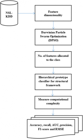
Here, the NSL-KDD dataset is used as the dataset uses 20% instances as training data with the overall 25, 192 instances, and the remaining samples are used as testing datasets with a total of 22, 544 instances. It has 42 attributes among them, 41 attributes are classified as four diverse classes. Figure 1 depicts the flow diagram of the proposed model.
1) Basic (B) features: TCP/IP connection attributes for detecting delays.
2) Traffic (T) features: Features are related to window interval and it possesses two well-known features like same service and same host. The service feature tests the total number of links for a certain time interval that possess the same services.
3) Host (H) features: Attributes are provided to assess the attacks that remain for 2 seconds. It analyzes the total connections towards the destination in 2 seconds.
4) Content (C) features: Attributes are recommended by domain knowledge with moment interval.
This dataset consists of four diverse (traffic) categories with 23 attack types and some features:
1) Denial of Service (DoS): The attackers use network resources and make it busy; thereby, the users (authoritative) cannot access the available resources.
2) User-to-Root (U2R): The passwords are sniffed and apply attack the host to access the legitimate user. Some vulnerability is applied to access the system.
3) Remote-to-Local (R2L): Messages are transmitted by the attackers over the remote location to the host by applies vulnerabilities.
Figure 1. Flow diagram of the proposed model
Table 1. Dataset records
|
Dataset |
Number of records |
|||||
|
Total |
Normal |
DoS |
Probe |
U2R |
R2L |
|
|
KDD (train + 20% samples) |
25, 192 |
13, 449 |
9234 |
2289 |
11 |
209 |
|
KDD training |
125, 973 |
67, 343 |
45, 927 |
11, 656 |
52 |
995 |
|
KDD testing |
22, 544 |
9711 |
7458 |
2421 |
200 |
2654 |
Table 2. Dataset labels and attributes
|
No. |
Label |
Name |
No. |
Label |
Name |
|
1 |
B |
Duration |
10 |
C |
hot |
|
2 |
B |
protocol_type |
11 |
C |
num_failed_logins |
|
3 |
B |
Service |
12 |
C |
Logged_in |
|
4 |
B |
src_bytes |
13 |
C |
num_compromised |
|
5 |
B |
dst_bytes |
14 |
C |
root_shell |
|
6 |
B |
Flag |
15 |
C |
su_attempted |
|
7 |
B |
Land |
16 |
C |
Num_root |
|
8 |
B |
wrong_fragment |
17 |
C |
Num_file_creations |
|
9 |
B |
urgent |
18 |
C |
Num_shell |
|
|
19 |
C |
Num_access_files |
||
|
20 |
C |
Num_outbound_cmds |
|||
|
21 |
C |
Is_hot_logins |
|||
|
22 |
C |
Is_guest_logins |
|||
|
No. |
Label |
Name |
No. |
Label |
Name |
|
23 |
T |
Count |
32 |
H |
dst_host_count |
|
24 |
T |
Serror_rate |
33 |
H |
Dst_host_srv_count |
|
25 |
T |
Rerror_rate |
34 |
H |
Dst_host_same_srv_rate |
|
26 |
T |
Same_srv_rate |
35 |
H |
Dst_host_diff_srv_rate |
|
27 |
T |
Diff_srv_rate |
36 |
H |
Dst_host_same_src_port_rate |
|
28 |
T |
Srv_count |
37 |
H |
Dst_host_srv_diff_host_rate |
|
29 |
T |
Srv_serror_rae |
38 |
H |
Dst_host_serror_rate |
|
30 |
T |
Srv_rerror_rate |
39 |
H |
Dst_host_srv_serror_rate |
|
31 |
T |
Srv_diff_host_rate |
40 |
H |
Dst_host_rerror_rate |
|
|
41 |
H |
Dst_host_srv_rerror_rate |
||
|
42 |
--- |
class |
|||
Table 3. Attack categories
|
Attacks |
Attacks in every category |
|
DoS |
Teardrop, smurf, pod, Neptune, land, back |
|
Probes |
Port sweep, nmap, ipsweep, satan |
|
R2L |
Warezmaster, multi-hop, warezclient, spy, phf, passwd, imap, ftp write |
|
U2R |
Root kit, perl, load module, buffer overflow |
Table 4. Attack Distribution
|
Attacks |
Training set |
% |
Testing set |
% |
|
DoS |
45927 |
3645 |
7460 |
3353 |
|
Probes |
11656 |
925 |
2421 |
1073 |
|
R2L |
995 |
78 |
2885 |
1279 |
|
U2R |
52 |
41 |
67 |
29 |
|
Total |
125973 |
100 |
22544 |
100 |
4) Probe: The network is being scanned by the attackers to capture the information and makes network violation. Table 1 and Table 2 depict the dataset records, labels, and attributes of the NSL-KDD dataset. Table 3 shows four different attack categories.
Table 4 depicts the training dataset composes 53% normal data against 0.78% and 0.041% of R2L and U2R respectively. Similarly, the testing dataset is composed of 43.07% of normal data against 12.79% of R2L and 0.29% U2R respectively. The dataset imbalance influences the classifier performance highly during the prediction of vulnerabilities over the CPS model. The imbalanced samples give minority data of any class (lesser samples) which includes the performance of the system with reduced prediction rate of minority classes.
3.2 Darwinian particle swarm optimization
To be specific, the model goal is to overcome the curse over feature dimensionality with the selection of optimal bands of the classifier model [31]. The selection of more appropriate features is a complex task encountered in the classification process. Thus, the feature selection process intends to maximize the overall accuracy and it expressed as in Eq. (1):
$Overall accuracy =\frac{\sum_{i}^{N_{c}} C_{i i}}{\sum_{i j}^{N_{c}} C_{i j}} * 100$ (1)
where, $C_{i j}$ is the number of features allocated to class $j^{\prime}$ that belongs to class ${ }^{\prime} i^{\prime}, C_{i i}$ specifies the number of features which is appropriately assigned to the class ${ }^{\prime} i^{\prime}$ and $N_{c}$ is the number of classes. Here, optimal features are chosen via an optimization process where the solution acquires a fitness value from the SVM classifier during sample validation. The optimization process is performed using PSO algorithms. The significance of the model helps to model diverse variations of PSO and pretends to overcome the drawbacks related to it. One among the model is Darwinian PSO (D-PSO) that runs various PSO algorithm parallel using a diverse swarm, natural selection mechanism, and testing problem. When the search intends to give the sub-optimal solution, the search is completely discarded [32]. The swarms are rewarded and stagnates are punished by particle elimination and reduction of swarm life. The novelty of the work relies on factional computation to manage the convergence rate. The fractional order considers the infinite number of features with local operators and memory of past events. The characteristics of this model well-suited with this phenomenon like dynamical particle trajectories [33]. The fractional computation is shown by ${ }^{\prime} t^{\prime}$, where the fitness value is used for the computation of particle success. Here, the movement of the particles ${ }^{\prime} n^{\prime}$ over multi-dimensional space based on velocity $\left(v_{n}(t)\right)$ and position $\left(x_{n}(t)\right)$ with huge dependency over global best $\left(g^{\prime}(t)\right)$ and local best $\left(x_{n}^{\prime}(t)\right)$. It is mathematically expressed as in Eq. (2) and Eq. (3):
$v_{n}^{s}[t+1]=w_{n}^{s}[t+1]+\rho_{1} r_{1}\left(g^{\prime}(t)-x_{n}^{s}[t]\right)$$+\rho_{2} r_{2}\left(x_{n}^{\prime}[t]-x_{n}^{s}[t]\right)$ (2)
$w_{n}^{s}[t+1]=\alpha v_{n}^{s}[t]+\frac{1}{2} \alpha(1-\alpha) v_{n}^{s}[t-1]$$+\frac{1}{6} \alpha(1-\alpha)(2-\alpha) v_{n}^{s}[t-2]$$+\frac{1}{24} \alpha(1-\alpha)(2-\alpha)(3-\alpha) v_{n}^{s}[t-3]$ (3)
The anticipated fractional computation model for feature selection performs parallel running of diverse swarms over the search space, where ${ }^{\prime} s^{\prime}$ is the number of the swarm. Here, ${ }^{\prime} \rho_{1}{ }^{\prime}$ and ${ }^{\prime} \rho_{2}^{\prime}$ coefficients are allocated weights with inertial global best and local bests while determining new velocity. ${ }^{\prime} \rho_{1}{ }^{\prime}$ and ${ }^{\prime} \rho_{2}{ }^{\prime}$ are typically constant integer values with cognitive and social components with $\rho_{1}+\rho_{2}<2$. Moreover, various outcomes are attained by allocating various values for all components. The fractional coefficient will influence the past events with the determination of newer velocity, i.e. $0<\alpha<1$. With $'\propto'$ smaller value, particles eliminate the prior events; therefore eliminating the system dynamically and suspected to stuck at local solutions. It is known as exploitation behavior. With higher values of $'\propto'$, particles show diversified behavior which facilitates exploration of some novel solutions and enhances the performance. It is known as exploration behavior. When the exploration level is extremely high, then the algorithm takes a long time to predict the global solutions where the value of $'\propto'$ ranges from 0.6-0.8. ${ }^{\prime} r_{1}{ }^{\prime}$ and ${ }^{\prime}r_{2}^{\prime}$ parameters are random vectors among 0 and 1. The objective of feature selection shows that the particle dimension should be equal to the number of features. The position dimension $\left[\operatorname{dim}\left(x_{n}[t]\right]\right.$ and velocity dimension $\left[\operatorname{dim}\left(v_{n}[t]\right]\right.$ is equal to the number of features, i.e. $\left[\operatorname{dim}\left(v_{n}[t]\right]=\left[\operatorname{dim}\left(x_{n}[t]\right]=l\right.\right.$. The particle velocity is represented with an $l$-dimensional vector. The particles specify the position of binary values, i.e. $' 0^{\prime}$ and $' 1 '$ where $' 0 '$ specifies absence of features and $' 1 '$ is feature occurrence. The particle updation is expressed as in Eq. (4):
$\Delta x_{n}^{s}[t+1]=\frac{1}{1+e^{-v_{n}^{s}[t+1]}}$ (4)
The particles specify the position in binary values, i.e. ${ }^{\prime} 0^{\prime}$ and ${ }^{\prime} 1^{\prime}$. It is specified as in Eq. (5):
$x_{n}^{s}[t+1]= \begin{cases}1 & \Delta x_{n}^{s}[t+1] \geq r_{x} \\ 0 & \Delta x_{n}^{s}[t+1]<r_{x}\end{cases}$ (5)
where, $r_{x}$ is the random dimensional vector with a random number among 0 and 1 . The particles move in multidimensional space based on the position $x_{n}^{s}[t]$ from the discrete-time system. Consider, that the attack scenario comprises 4 categories, i.e $l=4$. It specifies that the particles are defined based on the current position and velocity in 4Dspace, i.e. $\operatorname{dim} v_{n}[t]=\operatorname{dim} x_{n}[t]=4$. It provides a straight ward understanding of the swarm particles. It is probable to observe the iterations and time $t=1$, the particle is eliminated with the elimination of the third position, i.e. $x_{1}[1]=[1101]$ where particle 2 eliminates the first and fourth band, i.e. $x_{2}[1]=[0110]$. The overall accuracy measure of these particles is represented as $65 \%$ and $69 \%$ for particles 1 and 2 specifically. Consider two particles where particle 2 is determined as the best performance of the swarm (See Figure determined as the best performance of the swarm (See Figure 2). Therefore, the particle 1 attraction induces particle velocity and position for successive iterations.
Figure 2. Fractional DPSO functionality
3.3 Case study
In the attack scenario, the application of the anticipated model relies on feature selection. Some shortcomings encountered in the existing models are addressed using this feature reduction model. Here, the attributes and the corresponding values are considered as threshold. The attributes give a wider range of threshold values modeled for feature bank evaluation. The anticipated feature selection approach predicts the most selective features based on classification accuracy with corresponding validation samples. The feature selection approach not only resolves the shortcomings of the existing approach; however, but also diminishes the feature redundancy and handles the curse of dimensionality. The preliminary workflow of the model is given as:
1) Construct the feature bank composed of raw input data and the attributes are attained based on the network flow.
2) In some cases, principal components, i.e. components with cumulative variance are maintained and features are considered to a certain range.
3) The raw data is concatenated into a stacked vector where the training samples are partitioned into two diverse categories: training and validation samples.
4) The anticipated feature selection model is applied and the fitness of the particles is computed by the overall prediction accuracy of SVM for sample validation. After the completion of a certain iteration, the feature selection model predicts the most essential information over the validation samples.
Figure 3. Hierarchical structural level framework
5) SVM is considered with the entire set of testing and training samples and the classification map is achieved.
Therefore, efficient classification is achieved and mapped. The classification process is discussed in the section given below (Figure 3).
It is observed that PCA can be substituted by other feature extraction approaches and gives promising outcomes to handle the disadvantages of prevailing approaches.
3.4 Hierarchal Prototype classifier for structural framework
The architectural model of the proposed classifier model is analyzed and the computational complexity of the model is reduced. Consider, $\{x\}=\left\{x_{1}, x_{2}, \ldots, x_{k}, \ldots\right\}$ is a data stream in ' $N$ ' dimensional samples with different classes and ' $K$ ' instances. The samples are subdivided into subsets and the class labels are $\{x\}_{K}^{i}=\left\{x_{1}^{i}, \ldots, x_{K}^{i}\right\}$. It is composed of pyramidal hierarchies and it is trained parallel with the data samples in a self-organized manner (See Figure 2). The hierarchical prototype model derives data indirect manner over a top-down manner. The upper layers of the hierarchical model include generalized information which is more representative and abstractive [34]. However, the lower-level layers also contain essential information and nearer to the observed values. The layers of the prototype model are connected with intermediate layers and specify the local peak of multi-modal data distribution [35]. The prototype layers are connected with one or more intermediate layers. The procedure of this model is to predict the prototypes and self-organize them hierarchically from training samples of the class separately. The observed samples of the classes $\left(x_{k}^{i}\left(k=1,2, \ldots, k^{i}, \ldots\right)\right.$ are normalized and expressed as in Eq. (6):
$x_{k}^{i}=\frac{x_{k}^{i}}{\left\|x_{k}^{i}\right\|}$ (6)
where, ||$x_{k}^{i}||=\sqrt{\sum_{j=1}^{N}\left(x_{k, j}^{i}\right)^{2}}$. It is a normalization process that converts the Euclidean distance among the samples in cosine dissimilarity distance measure and the outcomes improve the competency of the HP classifier model for dealing with high-dimensional complex issues. The preliminary sample with $i t h$ class is adopted for predicting the hierarchical model and considers it as the prototype for all layers. It is given as in Eq. (7):
$M_{l}^{i} \rightarrow 1 ; p_{l, m_{l}^{i}}^{i} \rightarrow x_{k^{i}}^{i} ; S_{l, M_{l}^{i}} \rightarrow 1$ (7)
where, $S_{l, M_{l}^{i}}$ is the number of samples related with $p_{l, m_{l}^{i}}^{i}$. The sub-ordinate relationships among the prototypes are established hierarchically. It is expressed as in Eq. (8):
$\mathcal{L}_{0}^{i} \rightarrow\left\{p_{1, M_{l}^{i}}^{i}\right\}$ (8)
The collections of the immediate subordinates are initialized using Eq. (9):
$\mathcal{L}_{0}^{i} \rightarrow\left\{p_{L, M_{l}^{i}}^{i}\right\}$ (9)
The hierarchical model is established and the resembling chain with $p_{1, M_{l}^{i}}^{i}$ is considered as starting node and $p_{L, M_{l}^{i}}^{i}$ is the ending node. The proposed classifier model is constantly selfevolving over the system level structural model and updates the meta-parameters over the streaming data under uncertain conditions. When the data samples $\left(x_{k}^{i}\left(K^{i} \rightarrow K^{i}+1\right)\right)$ are observed and the system updates the process is initiated from the topmost layer. Initially, the prototypes are identified via the following expression Eq. (10):
$\eta_{l}^{*}= \begin{cases}\arg \max _{p \in \mathcal{L}_{0}^{i}}\left(\left(x_{K^{i}}^{i}-p \|\right.\right. & \text { if } l=1 \\ \arg \max _{p \in \mathcal{L}_{-}\left(l-1, n_{l-1}^{*}\right.}\left(\left(x_{K^{i}}^{i}-p \|\right.\right. & \text { if } l=2,3, \ldots, L\end{cases}$ (10)
It is observed that the proposed hierarchical structural model predicts the number of prototypes with the learning process where complex problems are considered inevitable. Based on the analysis, Eq. (10) drastically enhances the computational efficiency of the prototype model by diminishing the searching range from the entire data space towards the small group of neighborhood prototypes. It drastically eliminates the computational resources as the majority of the prototypes are away from $x_{K i}^{i}$ the anticipated model predicts the nearest prototype effectively compared to alternative models. During the validation process, the classifier model describes the class labels of the given sample. Here, the layers of the classifier are considered for classification purposes. The upper layers are more representative and adopted for coarse and efficient classification purposes. However, the lower level possesses essential information and it is adopted for performing effectual classification process.
Figure 4. Layered hierarchical architecture
Consider the $l^{\text {th }}$ layer of $(l=1,2, \ldots, L)$ which is used for certain unlabelled data samples specified by $x_{k}$ with the local decision-making process in a hierarchical manner (See Figure 4). It helps to produce the confidence score $\lambda^{i}\left(x_{k}\right)$ is based on the similarity among $x_{k}$ and the nearest prototypes are chosen at the initial layer with 'nearest prototype'. Two optimal searching methods are used for computation and it is expressed as in Eq. (11):
$\lambda^{i}\left(x_{K}\right)=\max _{p \in\{p\}_{l}^{i}} e^{-|| p-x_{k}||^{2}}$ (11)
where, $\{p\}_{l}^{i}=\left\{p_{l, 1}^{i}, p_{l, 2}^{i}, \ldots, p_{l, M_{l}^{i}}^{i}\right\}$ specifies the collective prototypes over the hierarchical layer. The hierarchies produce confidence score on $x_{k}$ and the class labels are determined as in Eq. (12) and Eq. (13):
$\operatorname{label}\left(x_{k}\right) \rightarrow$ class $i *$ (12)
$i^{*} \rightarrow \arg \max _{i=1,2, \ldots, C}\left(\lambda^{i}\left(X_{k}\right)\right)$ (13)
It is essential to analyze the mode with high computational efficiency as the upper layers are utilized for classification purposes as the layers possess a smaller amount of generalized prototypes. The computational efficiency of the classifier is reduced as the layers are composed of a huge amount of prototypes, high-dimensional and large-scale problems. For certain unlabelled samples, sometimes wrong decisions are made over the top-down searching process. Assume that the $l^{t h}$ layer of the proposed classifier model is used for classification purposes. During the validation process (unlabelled data samples), the hierarchical model produces the confidence score based on similarity measures. The computational complexity is given as $O\left(N \sum_{i=1}^{C}\left(M_{0}^{i}+\sum_{j=1}^{l-1} P_{j, n_{j}^{*}}^{i}\right.\right.$. During the high dimensional and large scale process, the computational is more efficient. While for small-scale problems, the model is more efficient with leaser computational complexity. The outcomes are validated using the numerical analysis which is discussed in the section given below.
|
Algorithm 1: |
|
Input: Data streams
|
This section discusses the outcome of the proposed model to measure the uncertainty that occurs in the CPS. Here, two essential processes are carried out and it is known as feature selection and classification process. The simulation is done in MATLAB simulation environment on Intel Pentium 4 processor, CPU 3.20 GHz, and 4 GB memory where the proposed intelligent hierarchical-level structural model provides security, access, and fulfils the QoS requirement efficiently. The performance of the hierarchical model is compared with various existing approaches like the Deep belief (DB) network model, Deep learning-based Recurrent Neural Networks, federated self-learning, federated transfer learning, and deep FED. Some performance metrics like accuracy, precision, recall, F1-score, ROC, error rate, execution time, and confusion matrix are evaluated. The uncertainty or fault that occurs over the network layer is measured with the iHLSF model. These metrics are expressed as in Eq. (14) – Eq. (19):
Accuracy $=\frac{T P+T N}{T P+T N+F P+F N}$ (14)
Recall $=\frac{T P}{T P+F N}$ (15)
AUC $=\int_{0}^{1} R O C(t) d t$ (16)
Precision $=\frac{T P}{T P+F P} * 100$ (17)
F1-score $=\frac{2 T P}{2 T P+F P+F N}$ (18)
RMSE $\left.=\sqrt{\left[\sum_{i=1}^{N}\left(y_{i}-x_{i}\right)^{2} / N\right.}\right]$ (19)
True positive (TP): the proposed hierarchical-level structural classifier needs to determine accurately the class feature to predict where the attack is identified.
True Negative (TN): the hierarchical-level structural classifier needs to determine the class features are negative accurately.
False Positive (FP): the hierarchical-level structural classifier inaccurately determines the normal traffic as an attack pattern.
False Negative (FN): The proposed hierarchical-level structural classifier incorrectly classifies the attack as normal traffic.
Table 5. Accuracy comparison
|
Iterations |
100 |
300 |
500 |
800 |
1000 |
|
DB |
79.45 |
82.33 |
90.25 |
95.6 |
99.4 |
|
Deep learning RNN |
60.35 |
68.9 |
72.55 |
81.96 |
86.9 |
|
federated self-learning |
70.11 |
76.25 |
81.22 |
86.99 |
99.09 |
|
federated transfer learning |
73.14 |
79.88 |
85.2 |
91.2 |
99.13 |
|
Deep FED |
75.55 |
80.36 |
87.48 |
92.33 |
99.20 |
|
iHLSF |
81.12 |
85.69 |
93.25 |
97.18 |
99.6 |
Table 6. Precision comparison
|
Iterations |
100 |
300 |
500 |
800 |
1000 |
|
DB |
83.65 |
88.74 |
92.44 |
96.87 |
100 |
|
federated self-learning |
71.44 |
76.2 |
82.51 |
90.66 |
98.86 |
|
federated transfer learning |
76.02 |
79.2 |
88.99 |
93.5 |
99.34 |
|
Deep FED |
81.06 |
83.99 |
87.25 |
93.65 |
98.86 |
|
iHLSF |
86.99 |
91.25 |
95.87 |
97.54 |
99 |
Table 7. Recall comparison
|
Iterations |
100 |
300 |
500 |
800 |
1000 |
|
DB |
81.45 |
82.33 |
89.96 |
91.25 |
99.5 |
|
federated self-learning |
71.25 |
78.54 |
82.69 |
89.41 |
96.76 |
|
federated transfer learning |
73.89 |
78.88 |
83.94 |
93.89 |
96.82 |
|
Deep FED |
76.58 |
80.11 |
85.62 |
89.7 |
97.36 |
|
iHLSF |
85.7 |
90.7 |
95.22 |
98.47 |
100 |
Table 8. F1-score comparison
|
Iterations |
100 |
300 |
500 |
800 |
1000 |
|
DB |
81.22 |
87.88 |
92.15 |
96.64 |
99.7 |
|
federated self-learning |
71.10 |
73.55 |
81.25 |
92.85 |
97.78 |
|
federated transfer learning |
73.25 |
78.5 |
86.9 |
93.2 |
98.03 |
|
Deep FED |
80.05 |
83.97 |
91.24 |
94.55 |
98.10 |
|
iHLSF |
86.74 |
92.33 |
96.21 |
98.53 |
99.85 |
The number of iterations for fractional DPSO based feature selection approaches is equal to 10. The proposed fractional DPSO model is considered as the randomized approach based on the population level that runs 30 times and outcomes are compared and the capabilities are measured. The parameters $\rho_{1}, \rho_{2}$ and $\propto$ are initialized by 0.9, 0.9, and 0.7 respectively. These sets of features are used by the NSL-KDD dataset for independent data distribution. The proposed feature selection model outcomes in better execution time are 8.2104 seconds and an error rate of 0.041 which is comparatively lesser than other approaches. The proposed fractional DPSO model is provided to measure the accuracy during sample validation. The classification accuracies are evaluated with outcomes from other feature selection approaches. The runs are sorted increasingly during validation samples. The significance of the proposed classifier model (independent variables) gives CPU processing time and final overall accuracy (dependent variables). Based on the analysis, it is observed that the traditional feature selection approaches are more feasible with relatively least dimensional cases. When the features are increased, the required statistical evaluation is considered in a non-wider manner. During the evaluation process, 100, 300, 500, 800, and 1000 iterations are considered.
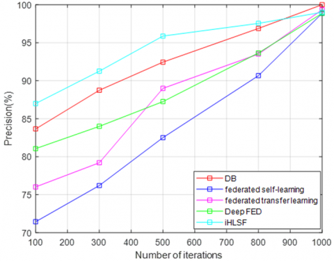
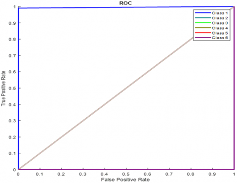
The accuracy is evaluated based on iterations. In the future, the models with future improved to enhance the accuracy rate. Table 5 depicts the accuracy of the proposed iHLSF model is 99.6% which is 0.2%, 12.7%, 0.51%, 0.47%, and 0.4% higher for proposed iHLSF model for 1000 iterations (See Figure 5). Table 6 depicts the precision of the proposed iHLSF model is 99% which is 1% lesser than DB, 0.14%, higher than federated self-learning, 0.34% lesser than federated transfer learning, and 0.14% lesser than deep FED for the proposed iHLSF model for 1000 iterations (See Figure 6). Table 7 depicts the F1-score of the proposed iHLSF model is 100% which is 0.5%, 3.24%, 3.18%, and 2.64% higher than an existing model for 1000 iterations (See Figure 7). Table 8 depicts the comparison of recall where the proposed iHLSF is 99.85%, 0.15%, 2.07%, 1.82%, and 1.75% higher than DB, federated self-learning model, federated transfer learning model, and deep FED model respectively (See Figure 8). Figure 9 depicts the confusion matrix of the proposed iHLSF classifier model for the target class and output class. Based on Figure 10, the ROC curve is plotted based on the True Positive Rate (TPR) and False Positive Rate (FPR). The plotting is done among these two metrics in a straight line for all the dataset classes where the values range from 0 to 1 respectively.
Figure 5. Accuracy comparison
Figure 6. Precision comparison
Figure 7. F1-score comparison
Figure 8. Recall comparison
Figure 9. Confusion matrix
Figure 10. ROC computation
From the extensive analysis, it is known that the anticipated model outperforms the existing approaches conventionally. The computational efficiency is higher for large-scale, high-dimensional, and complex CPS problems. It is considered as the unique hierarchical level structural model to measure the uncertainty that occurs over the network layer of the CPS system. The vulnerabilities show huge influence over the system model. The proposed classifier model is competent to deal with complex issues at various levels of granularity and learns the results. The classifier model facilitates the user to determine the number of structural levels and selects it as a suitable model for decision making. This model is strongly feasible and strengthens the ability of the model over real-time applications. Thus, the classifier model gives a stronger alternative to the conventional approaches. It is highly attractive for large-scale CPS problems.
Here, an intelligent hierarchical level structural framework is proposed for classifying the threat over the CPS system. The model intends to reduce the dimensionality curse and manages the convergence rate. The fractional DPSO model automatically selects the influencing features to improve classification accuracy. The model works faster than the existing approaches during the evaluation of the probability of the class labels. The model fulfils the research objective by improving the security-level, access-level, and QoS requirements and reduces the computational complexity. Also, the model visualizes the uncertainties and the vulnerability using the NSL-KDD dataset. The model gives 99.6% accuracy, 99% precision, 100% recall and 99.86% F1-score. However, some issues need to be addressed in the future as there is no scientific way to determine the layers of the classifier model to work efficiently over certain CPS problems.
[1] Lee, E.A. (2008). Cyber-physical systems: Design challenges. 2008 11th IEEE International Symposium on Object and Component-Oriented Real-Time Distributed Computing (ISORC), Orlando, FL, USA, pp. 363-369. http://dx.doi.org/10.1109/ISORC.2008.25
[2] Ding, D., Han, Q. L., Xiang, Y., Ge, X., Zhang, X.M. (2018). A survey on security control and attack detection for industrial cyber-physical systems. Neurocomputing, 275: 1674-1683. http://dx.doi.org/10.1016/j.neucom.2017.10.009
[3] Han, S., Xie, M., Chen, H.H., Ling, Y. (2014). Intrusion detection in cyber-physical systems: Techniques and challenges. IEEE Systems Journal, 8(4): 1052-1062. https://doi.org/10.1109/JSYST.2013.2257594
[4] Abeshu, A., Chilamkurti, N. (2018). Deep learning: The frontier for distributed attack detection in fog-to-things computing. IEEE Communications Magazine, 56(2): 169-175. http://dx.doi.org/10.1109/MCOM.2018.1700332
[5] Vigneswaran, R.K., Vinayakumar, R., Soman, K.P., Poornachandran, P. (2018). Evaluating shallow and deep neural networks for network intrusion detection systems in cyber security. In 2018 9th International Conference on Computing, Communication and Networking Technologies (ICCCNT), Bengaluru, India, pp. 1-6. http://dx.doi.org/10.1109/ICCCNT.2018.8494096
[6] Schlegl, T., Seeböck, P., Waldstein, S.M., Langs, G., Schmidt-Erfurth, U. (2019). f-AnoGAN: Fast unsupervised anomaly detection with generative adversarial networks. Medical Image Analysis, 54: 30-44. http://dx.doi.org/10.1016/j.media.2019.01.010
[7] Goh, J., Adepu, S., Tan, M., Lee, Z.S. (2017). Anomaly detection in cyber physical systems using recurrent neural networks. In 2017 IEEE 18th International Symposium on High Assurance Systems Engineering (HASE), Singapore, pp. 140-145. http://dx.doi.org/10.1109/HASE.2017.36
[8] Khamfroush, H., Bartolini, N., La Porta, T.F., Swami, A., Dillman, J. (2016). On propagation of phenomena in interdependent networks. IEEE Transactions on Network Science and Engineering, 3(4): 225-239. http://dx.doi.org/10.1109/TNSE.2016.2600033
[9] Buldyrev, S.V., Shere, N.W., Cwilich, G.A. (2011). Interdependent networks with identical degrees of mutually dependent nodes. Physical Review E, 83: 016112. http://dx.doi.org/10.1103/PhysRevE.83.016112
[10] Huang, Z., Wang, C., Nayak, A., Stojmenovic, I. (2014). Small cluster in cyber physical systems: Network topology, interdependence and cascading failures. IEEE Transactions on Parallel and Distributed Systems, 26(8): 2340-2351. http://dx.doi.org/10.1109/TPDS.2014.2342740
[11] Lu, C., Saifullah, A., Li, B., et al. (2015). Real-time wireless sensor-actuator networks for industrial cyber-physical systems. Proceedings of the IEEE, 104(5): 1013-1024. http://dx.doi.org/10.1109/JPROC.2015.2497161
[12] Chen, C., Yan, J., Lu, N., Wang, Y., Yang, X., Guan, X. (2015). Ubiquitous monitoring for industrial cyber-physical systems over relay-assisted wireless sensor networks. IEEE Transactions on Emerging Topics in Computing, 3(3): 352-362. http://dx.doi.org/10.1109/TETC.2014.2386615
[13] Li, B., Lu, R., Wang, W., Choo, K.K.R. (2016). DDOA: A dirichlet-based detection scheme for opportunistic attacks in smart grid cyber-physical system. IEEE Transactions on Information Forensics and Security, 11(11): 2415-2425. http://dx.doi.org/10.1109/TIFS.2016.2576898
[14] Qiu, C., Yu, F.R., Yao, H., Jiang, C., Xu, F., Zhao, C. (2018). Blockchain-based software-defined industrial Internet of Things: A dueling deep Q-learning approach. IEEE Internet of Things Journal, 6(3): 4627-4639. https://doi.org/10.1109/JIOT.2018.2871394
[15] Ismail, M., Shaaban, M.F., Naidu, M., Serpedin, E. (2020). Deep learning detection of electricity theft cyber-attacks in renewable distributed generation. IEEE Transactions on Smart Grid, 11(4): 3428-3437. http://dx.doi.org/10.1109/TSG.2020.2973681
[16] Wang, H., Ruan, J., Wang, G., Zhou, B., Liu, Y., Fu, X., Peng, J. (2018). Deep learning-based interval state estimation of AC smart grids against sparse cyber attacks. IEEE Transactions on Industrial Informatics, 14(11): 4766-4778. http://dx.doi.org/10.1109/TII.2018.2804669
[17] Liu, J., Zhang, W., Ma, T., Tang, Z., Xie, Y., Gui, W., Niyoyita, J.P. (2020). Toward security monitoring of industrial cyber-physical systems via hierarchically distributed intrusion detection. Expert Systems with Applications, 158: 113578. http://dx.doi.org/10.1016/j.eswa.2020.113578
[18] Preuveneers, D., Rimmer, V., Tsingenopoulos, I., Spooren, J., Joosen, W., Ilie-Zudor, E. (2018). Chained anomaly detection models for federated learning: An intrusion detection case study. Applied Sciences, 8(12): 2663. http://dx.doi.org/10.3390/app8122663
[19] Zhao, Y., Chen, J., Wu, D., Teng, J., Yu, S. (2019). Multi-task network anomaly detection using federated learning,” In Proc. International Symposium on Information and Communication Technology (SoICT), Hanoi HaLong Bay, Vietnam, pp. 273-279. http://dx.doi.org/10.1145/3368926.3369705
[20] Chen, Y., Zhang, J., Yeo, C.K. (2019). Network anomaly detection using federated deep autoencoding Gaussian mixture model. In Proc. International Conference on Machine Learning for Networking (MLN), Paris, France, pp. 1-14. http://dx.doi.org/10.1007/978-3-030-45778-5_1
[21] Schneble, W., Thamilarasu, G. (2019). Attack detection using federated learning in medical cyber-physical systems. In Proc. International Conference on Computer Communications and Networks (ICCCN), Valencia, Spain, pp. 1-8.
[22] Loukas, G., Gan, D., Vuong, T. (2013). A review of cyber threats and defence approaches in emergency management. Future Internet, 5(2): 205-236. http://dx.doi.org/10.3390/fi5020205
[23] Chakraborty, S., Sharma, R.K., Tewari, P. (2017). Application of soft computing techniques over hard computing techniques: A survey. International Journal of Indestructible Mathematics & Computing, 1(1): 8-17. http://dx.doi.org/10.18510/ijsrtm.2017.542
[24] Shi, J., Wan, J., Yan, H., Suo, H. (2011). A survey of cyber-physical systems. In 2011 International Conference on Wireless Communications and Signal Processing (WCSP), Nanjing, China, pp. 1-6. http://dx.doi.org/10.1109/WCSP.2011.6096958
[25] Khaitan, S.K., McCalley, J.D. (2014). Design techniques and applications of cyberphysical systems: A survey. IEEE Systems Journal, 9(2): 350-365. http://dx.doi.org/10.1109/JSYST.2014.2322503
[26] Wang, J., Abid, H., Lee, S., Shu, L., Xia, F. (2011). A secured health care application architecture for cyber-physical systems. arXiv preprint arXiv:1201.0213.
[27] Zhu, Q., Basar, T. (2015). Game-theoretic methods for robustness, security, and resilience of cyberphysical control systems: games-in-games principle for optimal cross-layer resilient control systems. IEEE Control Systems Magazine, 35(1): 46-65. https://doi.org/10.1109/MCS.2014.2364710
[28] Mitchell, R., Chen, R. (2015). Modeling and analysis of attacks and counter defense mechanisms for cyber physical systems. IEEE Transactions on Reliability, 65(1): 350-358. http://dx.doi.org/10.1109/TR.2015.2406860
[29] Engel, M., Schmoll, F., Heinig, A., Marwedel, P. (2011). Unreliable yet useful–reliability annotations for data in cyber-physical systems. INFORMATIK 2011-Informatik schafft Communities.
[30] Davis, K.R., Davis, C.M., Zonouz, S.A., Bobba, R.B., Berthier, R., Garcia, L., Sauer, P.W. (2015). A cyber-physical modeling and assessment framework for power grid infrastructures. IEEE Transactions on Smart Grid, 6(5): 2464-2475. http://dx.doi.org/10.1109/TSG.2015.2424155
[31] Daamouche, A., Melgani, F., Alajlan, N., Conci, N. (2013). Swarm optimization of structuring elements for VHR image classification. IEEE Geoscience and Remote Sensing Letters, 10(6): 1334-1338. http://dx.doi.org/10.1109/LGRS.2013.2240649
[32] Tillett, J., Rao, T., Sahin, F., Rao, R. (2005). Darwinian particle swarm optimization. RIT Scholar Works.
[33] Sindhu, S.S.S., Geetha, S., Kannan, A. (2012). Decision tree based light weight intrusion detection using a wrapper approach. Expert Systems with Applications, 39(1): 129-141. http://dx.doi.org/10.1016/j.eswa.2011.06.013
[34] Xia, G.S., Hu, J., Hu, F., et al. (2017). AID: A benchmark data set for performance evaluation of aerial scene classification. IEEE Transactions on Geoscience and Remote Sensing, 55(7): 3965-3981. http://dx.doi.org/10.1109/TGRS.2017.2685945
[35] Gu, X., Angelov, P.P., Zhang, C., Atkinson, P.M. (2018). A massively parallel deep rule-based ensemble classifier for remote sensing scenes. IEEE Geoscience and Remote Sensing Letters, 15(3): 345-349. http://dx.doi.org/10.1109/LGRS.2017.2787421