Mohammad Reza Mazinani | Kourosh Dadashtabar Ahmadi*
© 2021 IIETA. This article is published by IIETA and is licensed under the CC BY 4.0 license (http://creativecommons.org/licenses/by/4.0/).
OPEN ACCESS
Many videos uploaded to online video platforms contain adult content that violates these platforms' policies and should be removed immediately. To recognize obscene videos, we developed a model that can process video frames in real-time while also adapting to time budget or hardware processing capacity. Thus, a deep convolutional neural network with multiple outputs was used. A decision-maker module was then designed to decide which neural network outputs to process and which label to assign to each frame. Using the reinforcement learning method, the decision-maker module is trained based on the results of previous frames as well as the results of neural network outputs while keeping the time budget in mind. Experiments showed that sacrificing a small amount of accuracy can increase speed by up to 4.7 times over the base model. We conclude that using a content correlation between consecutive frames not only reduces processing time by eliminating unnecessary frame processing but also improves the accuracy of the frame classification. It was also discovered that while using more of the previous frames, increases processing speed, the error in classifying the frame increases when the scene is changed.
porn frame detection, adult video recognition, real-time video processing, convolutional neural network, adaptive classification, computer vision
Broadcasting and watching online videos have expanded dramatically as people's access to high-speed and stable internet has increased. Some users broadcast nude or porn content in online broadcasting services to attract viewers in violation of the rules of the service. In addition, some scenes in the released movies and tv series may contain adult content. Therefore, it is very useful to detect and filter adult scenes from movies and tv series being played on home devices. Due to a large number of these videos, many experts have attempted to detect adult scenes automatically with high accuracy and speed [1, 2].
In order to design efficient models for recognizing adult scenes in a video, two major issues must be addressed: real-time processing and model adaptability. The acceptable delay to the user in live video playback is a few seconds at most. Therefore, the processing of these videos should be quick and in real-time. An adaptive model means being able to adapt to the given requirements. Our proposed model, in particular, is intended to perform best under various time constraints. For example, when the processing server is overwhelmed by a large number of broadcasting users, the time allotted for each video is reduced, and our model can adapt to this need and process videos with a slight reduction in accuracy without significant delay.
Detecting porn frames in videos on various online platforms presents numerous challenges. As the camera moves, the frames blur, and their contents are not easily recognizable. Also, videos produced by amateur users do not have proper lighting, and sometimes they intentionally try to hide the pornographic portions of the video between normal parts of the video. Furthermore, each video contains a large number of frames, which quickly and accurately process all frames is very time-consuming. In contrast, there are two features in the video that can be used to accelerate the processing of frames. There is a semantic relationship between consecutive video frames, and identifying each frame can aid in identifying subsequent frames. Furthermore, not all frames in a video are equally difficult, and some frames can be processed quickly using light and fast Convolutional neural networks (CNN).
Three steps are involved in analyzing adult content in a video:
Extracting and selecting frames: To increase speed, Moustafa [3] extracts the video keyframes and only processes them. Wehrmann et al. [4] use the Long Short-Term Memory (LSTM) network to process all frames sequentially. In our method, we intelligently and adaptively select some frames for processing based on the time budget and label the remaining frames using the previous frames.
Frame classification: In some methods, hand-crafted features were used to classify pornographic or violent frames [5-8]. CNN are used in the majority of methods today [1, 3, 9, 10]. We also used a CNN with several outputs from the middle layers to classify video frames due to the high accuracy of deep networks.
Decision: Some methods detect porn video frames and, if there are more than a certain number of porn frames, classify the entire video as porn [3, 10]. Mallmann et al. [11] process video frames in real-time, and blur the pornographic parts of each frame. Our method's goal is also to find and filter pornographic frames among normal video frames.
To design the final model, we used a CNN that has four outputs from middle layers. Then we designed a decision-maker module that determines the frame processing path for each video frame by viewing the current and previous frames. The decision-making module is trained using the reinforcement learning algorithm to choose the best CNN output for processing based on the given time budget. We describe our contributions below:
The smart selection of frames: Methods that only process keyframes may make mistakes in keyframe extraction. Furthermore, an error in the classification of each keyframe causes all surrounding frames to be labeled incorrectly. Our model considers all frames and only fully processes a sufficient number of frames if necessary, deciding on the label of the remaining frames with less processing.
Using past frames information to process the current frame more accurately: There is a huge semantic correlation between consecutive video frames. When the previous frames were processed in our model, the model can process the current frame faster and with lighter parts of the CNN, taking into account the information from the previous frames.
Adaptable to time budget or hardware processing capability: When the budget is limited, the model employs lighter parts of the CNN and processes each frame faster by sacrificing a small amount of accuracy. The model can also adapt to slower processing hardware and produce the appropriate accuracy for real-time processing. For example, our algorithm can process programs that are being played on TVs with limited processing power.
The rest of this paper is structured as follows. Section 2 discusses some of the work in the field of adult image and video classification, as well as work to accelerate video processing and CNN networks. Section 3 describes the model's overall structure before delving into the specifics of each of its modules. Section 4 introduces the dataset used, followed by an examination of the implementation details and results obtained. Section 5 concludes the work and establishes guidelines for future works.
2.1 Porn image and video recognition
The early methods of recognizing adult images used hand-crafted features, such as color, skin, face, and texture [12-14]. Some articles used the same methods to classify adult videos [5, 6]. In addition to low accuracy in image recognition, these methods also consumed a lot of processing time. Hartatik et al. [15] presented methods that use low-level features like scale-invariant feature transform (SIFT) and speeded up robust features (SURF). These methods are a little more accurate than previous methods in addition to the possibility of classifying non-color images.
Many algorithms today use deep learning methods to classify images due to their high accuracy. Mahadeokar and Pesavento [16] provided an online tool to identify Not-Safe-For-Work (NSFW) images called Yahoo Detector. They fine-tuned the RezNet50 [17] network, previously trained on the ImageNet [18] dataset. Yuan and Zhang [10] used the same network structure to identify porn scenes on live broadcast platforms. These articles show that the CNN methods are far more accurate than previous methods.
In addition to the single frame features, certain articles used other features to enhance the accuracy of porn video classification. Perez et al. [9] use both static and motion features for CNN-based classification of videos. Wang et al. [1] use spatial, audio, motion, and temporal feature in live video by a multi-modal deep network. They also used the text of user comments next to the streaming videos. Adding these new features greatly increases the accuracy of video classification, but the classification time increases accordingly.
2.2 Speed-up video recognition
CNN processing time is high on conventional CPUs, and as network depth is increased to improve network accuracy, this processing time increases. Videos also have a high number of frames per second, which takes a long time to process.
Many articles, rather than processing all of the frames of a video, extract several keyframes from it and classify the entire video based on the keyframes label [3, 19]. With this solution, the processing speed will increase, but if the goal is to accurately find the porn frames in a video, the overall detection accuracy will be very low.
Devani et al. [7] distribute video frame chunks between multiple GPUs to enable real-time processing of the online video and filter porn video. In this manner, frames are processed in parallel. The parallel processing method increases the processing capacity and can be applied to most frame processing methods such as our proposed model.
Shen et al. [20] combined the costly but complete Oracle model with a less costly and fast compact model. They built a cascade classifier so that if its input belongs to one of the frequent classes in the video frame distribution, it returns quickly with the compact model's classification result; otherwise, it invokes the Oracle model. One of the drawbacks of this method is that if the frame is not classified by the compact model, it must be processed by the Oracle model from the beginning.
2.3 Speed-up CNN classifier
To improve the speed of static CNN, networks with lighter structures have been proposed. These networks, in addition to being faster, can also be implemented on low-processing power hardware [21-24].
Input-dependent methods have also been proposed to increase the processing speed of images in deep convolutional networks. For different input images, Bengio et al. [25] remove unnecessary nodes from the layers, it is like drop-out nodes in CNN but in an input-dependent way. Lin et al. try to eliminate some CNN layers to reduce computation. Using the reinforcement learning method, they pruned the CNN layer by layer [26, 27]. The agent evaluates each convolutional kernel's importance and performs channel-wise pruning based on different samples. Berestizshevsky and Even [28] built a cascading structure using several outputs from the CNN middle layers, and at each output, the processing of each sample is terminated if its accuracy exceeds a threshold value. Bolukbasi et al. [29] used a CNN with multiple outputs from the middle layers. The module then decides whether to continue or stop image processing based on each output result. This way, images that are correctly classified in the first layers will not go to the next layers. In the Mazinani et al. [30] method, a selector module selects one of the CNN outputs for processing based on the time budget given for each image, and after viewing the result, determines a new output for processing if necessary.
3.1 Model overview
We present an adaptive method for real-time classifying video frames. We show video frames processing time for our model as follow:
EvaluationTime $\left(t^{\prime}\right)=$$\sum_{n=1}^{N} F_{n}\left(t^{\prime}\right) \cdot T\left(x_{n} \mid t^{\prime}, x_{n-1}\right)+T_{\text {Decision-maker }}\left(t^{\prime}\right)$ (1)
$F_{n}\left(t^{\prime}\right)= \begin{cases}1 & n-\text { th frame processed } \\ 0 & n-\text { th frame not processed }\end{cases}$ (2)
where, EvaluationTime $\left(t^{\prime}\right)$ is the total processing time for all frames given time budget $t^{\prime}, N$ is the number of video frames, $F_{n}\left(t^{\prime}\right)$ is the coefficient that determines whether the frame number $n$ needs to be processed or not. If the time budget is limited, the decision-maker estimates the label of some frames using the previous frame, and sets the $F_{n}\left(t^{\prime}\right)$ coefficient for the frame $n$ to $0 . T\left(x_{n} \mid t^{\prime}, x_{n-1}\right)$ is the classifier processing time for input frame $x_{n}$ given previous frame $x_{n-1}$, and time budget $t^{\prime}$, and $T_{\text {Decision-maker }}\left(t^{\prime}\right)$ is processing time of our decision-maker module given time budget $t^{\prime}$. The decision-maker at runtime is defined as a series of rules that are very fast and its processing time can be ignored.
Another way to reduce processing time is to use the method proposed by X. In this method, the CNN classifier uses only part of its layers to process simpler frames, thus reduce overall processing time. In addition to the difficulty and ease of the frame, our decision-maker also considers the previous frames’ labels, so the need to process the CNN layers will be even less. The general processing time of each frame $T\left(x_{n} \mid t^{\prime}, x_{n-1}\right)$ in our model is shown below.
$T\left(x_{n} \mid t^{\prime}, x_{n-1}\right)=\sum_{l=1}^{L} P_{l}\left(x_{n} \mid t^{\prime}, x_{n-1}\right) \cdot T_{l}$ (3)
$P_{l}\left(x_{n} \mid t^{\prime}, x_{n-1}\right)= \begin{cases}1 & l-\text { th layer processed } \\ 0 & l-t h \text { layer not processed }\end{cases}$ (4)
where, $L$ is the number of $\mathrm{CNN}$ layers, $T_{l}$ is the processing time of the $l-t h$ layer, and $P_{l}\left(x_{n} \mid t^{\prime}, x_{n-1}\right)$ is the coefficient that determines whether the $l-t h$ layer needs to be processed or not. If we want to use the maximum CNN capability, this coefficient is equal to 1 for all layers, and therefore all layers are processed, but in simpler frames, this coefficient can be 0 for many layers.
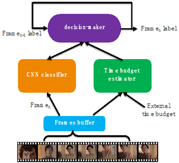
The final model consists of three main modules, which are shown in Figure 1. The first module is the time budget estimator, which specifies the time budget required for real-time processing based on hardware limitations and subsequent unprocessed frames. We describe its detail in Section 3.2. The next module is the CNN classifier. This classifier gets input frames and specifies its label, but unlike other CNNs, it has four different outputs, each with different accuracy and processing times. The specifications of our CNN classifier are described in Section 3.3. The principal module of our model is the decision-maker. This module specifies the final video frame label, based on observing the previous frames label, the CNN different outputs, and time budget. Our decision-maker is a reinforcement learning agent; We describe its algorithm in Section 3.4.
3.2 Time budget estimator
The time budget estimator module determines the $t^{\prime}$ value in Eq. (1) so that the entire video can be processed in real-time. $t^{\prime}$ is the average time given for processing each frame, and we specify this value as follows:
$t^{\prime}=$ Min (External time budget, Frame buffer budget) (5)
Frame buffer budget $=\frac{\text { Frame tolerable delay }-\text { Remaining frames }}{\text { video frame rate }}$ (6)
Here, the External time budget is a budget that is determined from outside the model. This value is determined based on the processing power of the hardware or the computational load sent to the server. For example, in an online streaming server, when the number of online users increases, the time budget for each video decreases so that there is no delay in processing the entire video. The Frame buffer budget is a time budget that assures us that video frames are processed with very low latency and in real-time. We set the total budget $t^{\prime}$ to the minimum of these two parameters so that we do not exceed any of these time constraints.
Figure 1. The overview structure of our real-time and adaptive model for porn frames detection in video
As shown in Figure 1, video streaming frames are first placed in a buffer and then sent to the CNN classifier for processing. The size of this buffer is determined based on the acceptable amount of frame delay in online video streaming. Frame tolerable delay is an acceptable number of frame delays in Eq. (6), and Remaining frames is the number of remaining frames in the buffer. The Frame buffer budget is obtained by dividing the remaining buffer capacity by the video frame rate. If the video frames are simple and fast to process, the buffer space will be emptier, and therefore more time budget will be available for processing the remaining frames.
3.3 CNN classifier
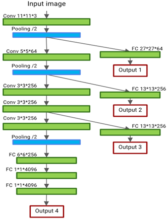
For the CNN classifier module, we used the network provided by Mazinani et al. [30]. The main structure of this network consists of the VGG-F network [31], then three outputs are added to its middle layers. We show the structure of the layers of this network in Figure 2.
Shallower outputs, such as Output 1 and Output 2, use fewer convolutional layers, so they are faster but less accurate. Instead, deeper outputs such as output 3 and output 4 are slower and more accurate.
Figure 2. CNN classifier structure presented by Mazinani et al. [30]
This network has four outputs, with the specifications for each layer written next to it. In the middle layer specifications, the first two numbers are the size of the filter, and the next number is the number of input channels.
3.4 Decision-maker
The decision-maker is the core of our model. It learns to controls the CNN classifier and to choose the best frame label. The decision-maker receives the time budget from the "time budget estimator" module. Considering the time budget, it performs three main tasks:
The decision-maker takes the result of the previous frames and decides whether the current frame needs to be processed. For example, if the time budget is very low and the classifier has chosen the previous frame label with high confidence, the decision-maker can estimate the current frame label without processing.
The decision-maker determines whether or not to process the frame further based on the outcome of the previous frames and the processed outputs from the CNN. For example, if the frame is processed with lighter parts of the CNN (early layers) and the label obtained in processing the current frame is the same as the previous frames label, the decision-maker can specify the result and terminate the processing.
Finally, the decision-maker selects the final frame label based on the previous frames label and the various network outputs. It should be noted that the CNN outputs and the output of the previous frames may differ. In this case, the decision-maker selects the most appropriate label based on prior experience.
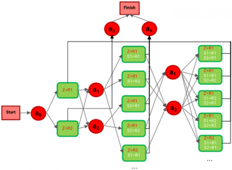
The designed decision-maker is a reinforcement learning agent, and we train it using the Q-learning algorithm. Figure 3 shows a simplified form of our reinforcement learning structure. The action $a_{0}$ refers to selecting the previous frame (Z). If this frame is labeled R1, the agent will enter the state Z = R1, otherwise it will enter the state Z = R2. In the next step, the agent can select one of the CNN outputs for processing (action $a_{1}$ and $a_{2}$) or specify the image label (action $a_{3}$ and $a_{4}$).
Figure 3. The simplified form of our reinforcement learning structure
The red circles represent actions, and the rectangles represent various states. In this simple model, it is assumed that the network has only two outputs. Also, only some states are shown as examples.
The concepts of action, state, and reward function will be explained in detail for a complete description of the decision-maker algorithm.
3.4.1 Action
Our agent can make different choices for processing or labeling frames. We have defined each of these choices as an action in our reinforcement learning model. Actions are divided into three categories: selecting previous frames, selecting CNN outputs, and selecting final labels. We show our actions as follows:
previous frames $=\left\{a_{0}, \ldots, a_{N Z-1}\right\}$
$C N N$ outputs $=\left\{a_{N Z}, \ldots, a_{N Z+N O-1}\right\}$
labels $=\left\{a_{N Z+N O}, \ldots, a_{N Z+N O+N C-1}\right\}$ (7)
where, NZ is the number of previous frames that the agent can consider, NO is the number of CNN output, and NC is the number of labels (classes). In our model the agent checks up to 3 previous frames (NZ=3), our CNN classifier has 4 outputs (NO=3), and the classes are divided into two labels, normal and porn (NC=2). So, the total number of actions is equal to NZ+NO+NC=9.
3.4.2 State
Based on the outcome of each action, we reach one of the states. For example, if the agent examines the previous frame, one of two different labels is selected. Therefore, each of these labels can be considered as a state. Also, for more accuracy, we consider the degree of confidence of the classifier to its output. For this purpose, a score is calculated for each label, and then, these scores are divided into four parts (Based on various trials and errors, the best number of parts is four). These parts are porn label with high confidence (R1), porn label with low confidence (R2), normal label with low confidence (R3), and normal label with high confidence (R4). In Section 3.5, we will explain how to calculate label scores in detail. We specify the middle states based on the actions as follows:
state $=\left\{S_{a_{0}}, S_{a_{1}}, \ldots, S_{a_{N Z+N O-1}}, S_{\text {Label }}\right\}$ (8)
$S_{a_{n}}=\{R 1, R 2, R 3, R 4, U N K N O W N\}$ (9)
$S_{\text {Label }}=\{$ porn, normal, $U N K N O W N\}$ (10)
where, $S_{a_{n}}$ specifies the states created by the $a_{n}$ action. By performing the actions, these states are determined with $R 1, R 2, R 3$, or $R 4$, otherwise, the states are determined with UNKNOWN. $S_{\text {Label }}$ specifies the states created by selecting the label porn or normal, and if the label is not selected this parameter is $U N K N O W N$.
Based on agent actions, we defined states. Agent actions include selecting one of the previous frames or CNN outputs, as well as selecting the frame label. Therefore, we show each state by Eq. (8). Each action, according to Eq. (9), generates a new state based on the output result. For example, when the agent selects the second output, the CNN result may be in the confidence range of R1, R2, etc., each of which creates a separate state. As a result, multiplying the number of different parts for each action yields the total number of states. Furthermore, as shown in Eq. (10) the new state is created based on the label selection, so all states must be multiplied by the number of labels plus $U N K N O W N$ label. The total number of states of our reinforcement learning model is:
$\begin{aligned} \text { Number of states } &=\left(N_{\text {parts }}+1\right)^{(N Z+N O)} \cdot\left(N_{\text {Label }}+1\right) \\ &=(4+1)^{(3+4)} \cdot(2+1)=234375 \end{aligned}$ (11)
where, $N_{\text {parts }}$ is the number of score parts, $N Z$ is the maximum number of previous frames that the agent can consider $(N Z=3), N O$ is the number of $\mathrm{CNN}$ output $(N O=$ 4), $N_{\text {Label }}$ is the number of labels $(N C=2)$. Because the number of states is 234375 , which is not a large number, training the reinforcement learning model can be accomplished using standard Q-learning methods.
3.4.3 Reward
The agent moves from one state to another by performing an action $a_{n}$. The agent receives a reward for the execution of this action and aims to maximize its overall reward. For this purpose, in the Q-learning algorithm, a value is defined for each pair of states and actions, which are stored in the q-table. In any state, by choosing the highest value, the highest reward can be achieved in the future steps. To train our model and update the values in the q-table, we use the following formula provided by Watkins and Dayan [32]:
$\begin{array}{ll}Q_{\text {new }} & \left(s_{t}, a_{t}\right) \leftarrow Q_{\text {old }}\left(s_{t}, a_{t}\right)+ \\ & \alpha \cdot\left(\text { Reward }_{t}+\gamma \cdot \max _{a} Q\left(s_{t+1}, a\right)-Q_{\text {old }}\left(s_{t}, a_{t}\right)\right)\end{array}$ (12)
Here, $Q\left(s_{t}, a_{t}\right)$ is the value in the q-table for pair of state $s_{t}$ and action $a_{t}$, coefficient $\alpha$ and $\gamma$ are learning rate and discount factor respectively, $\max _{a} Q\left(s_{t+1}, a\right)$ is the estimate of optimal future value from state $s_{t+1}$, and Reward $_{t}$ is the reward achieved by taking action $a_{t}$ in state $s_{t}$. We used the idea used $[30,33]$ to consider the accuracy and the processing time of the algorithm at the same time. Therefore, we define our reward function as follows:
Reward $_{t}=$ label correctness $_{t}-\lambda$.process time $_{t}$ (13)
We show the processing time of executing each action $a_{t}$ from state $s_{t}$ with the process time $_{t}$. Since the past frame has already been processed, executing $a_{0}$ does not cost time. Also, choosing a frame label does not cost much time. In these two cases, process timet=0. But when one of the $\mathrm{CNN}$ outputs is chosen for processing, convolution layers need to be processed, which includes the main processing time of the frame. Deeper CNN outputs contain more layers and therefore more processing time. In each state, if actions $a_{6}$ or $a_{7}$ are chosen, the final frame label is selected by the agent. If this selection is correct, we set the label correctnesst value to a positive constant number and otherwise to a negative constant number. The $\lambda$ coefficient determines the trade-off between processing time and processing accuracy. As the $\lambda$ coefficient increases, the importance of processing time increases, the model is trained to be faster but its accuracy is slightly reduced.
3.5 Scoring method
In addition to what label the classifier assigns to each frame, the classifier's degree of confidence in the declared label is also important. At each CNN output, there is a layer called SoftMax that assigns a probability to each label. Berestizshevsky and Even [28] suggest that this probability can be considered as the network's confidence in its output. Since the direct use of this probability number greatly increases the number of states, it is necessary to quantize these values. Different values (such as: 60%, 70%, 80% and 90%) were tested for the confidence interval division threshold on the test data and the best threshold value was selected between these values. So, for each label, we assign the probability of greater than 70% as high confidence and less as low confidence.
The agent selects CNN outputs then by observing the SoftMax layer, it obtains the confidence value in addition to the label. But the agent faces two major problems in examining the past frames.
Since the previous frames label was chosen by the decision-maker module, it does not have a score or a confidence value.
If we use only the assigned label, the probability of propagating an error will be very high. We know that the label of a frame is most likely the same as the label of the previous frames. The agent also considers this information according to the observation of training data. If the time budget is low, the agent will use the selected label from the previous frame. If the agent selects the wrong label for the previous frame, it will also make a mistake in selecting the current frame label. The same goes for error propagation for subsequent frames.
To solve the stated problems, the agent checks the previous frames and considers the label, only if it is obtained by calculating the outputs of the CNN. This reduces the possibility of error propagation.
Also, to obtain the value of confidence, the agent considers the confidence of the deepest CNN output as the confidence of the previous frames. The accuracy of lighter layers is lower than deeper layers, and the confidence expressed by them is also less accurate. Therefore, we define a scoring function to consider the accuracy of each CNN output. The accuracy of each CNN output is its accuracy on the validation dataset. The scoring function is described below:
Score $=\left(\left(\right.\right.$ sample $\left._{i}-0.5\right) *\left(\right.$ out $\left.\left.A c c_{o}+1-\max A c c\right)\right)$$+0.5$ (14)
where, sample $_{i}$ is the value of softmax output for sample $i$, out $A c c_{o}$ is the accuracy for output $c$ of the $\mathrm{CNN}$, and $\max A c c$ is the accuracy of the deepest layer of the CNN. The deepest layer has the maximum accuracy and by this equation, we don't penalize it. According to this equation, the less accurate a network output is, the more it will be penalized and the lower the score for that output. If the output value of the SoftMax layer is higher than $0.5$, the label is porn otherwise the label is normal. Therefore, before applying the penalty, we normalize the output value of the SoftMax layer between $-0.5$ and $+5$. The results of the scoring method will be shown in Section 4.3.
4.1 Dataset
We used the Noktedan [34] dataset to train our CNN. This dataset consists of 18,000 challenging images from around the web and social networks. Photos for the dataset were chosen to contain both simple and hard-to-classify images. We expanded this dataset to 30,800 images by adding frames from various movies and TV series. Which is divided into two sets: training set including 22,200 images and test set including 8,600 images.
To train and test the decision-maker model, we need a set of consecutive frames. So, we collected videos from movies and TV series. These videos were chosen from movies intended for mature, adult audiences, and some of them contain sexual content. The video dataset contains a total of 182,200 frames, 85,800 of which were extracted from the training set videos and 96,400 from the test set videos.
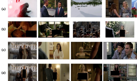
Figure 4. Examples of frames in image and video dataset. Rows (a) and (c) show the normal class, and rows (b) and (d) show the porn class
Figure 4 shows examples of frames in the dataset. In row (a) where normal frames are shown, some frames are very easily recognized. For example, an image with no humans and is clear is placed in the normal class with minimal processing. Some frames, however, are more difficult to recognize, such as those in which the camera is moving and the image is blurred. Some of the images in row (b) are simple, while others aren't. For example, it is more difficult to recognize those in crowded areas where only a small portion of the image contains a nude image, or in a dark frame where pornographic parts are not visible. Columns in rows (c) and (d) show frames from a video that first the frame is in the normal class and after a few frames by moving the actor or changing clothes or moving the camera, the frame is changed and placed in the porn class. The dataset can be downloaded from here (https://doi.org/10.6084/m9.figshare.14495367.v1).
4.2 CNN classifier training
The image dataset was used to train the CNN classifier. We used the weights of a previously trained network (trained with the Noktedan [34] dataset) to fine-tune this network with our new data. We resized all of the images to 224x224 and used the data augmentation technique to improve CNN training. Table 1 displays the test results of different network outputs on test data from the image dataset.
Table 1. The accuracy and the processing time of the CNN outputs on test data on the image dataset
|
Output name |
Accuracy (%) |
Time (ms) |
|
Output 1 |
72.8 |
4.65 |
|
Output 2 |
78.2 |
12.03 |
|
Output 3 |
83.0 |
17.27 |
|
Output 4 |
86.8 |
33.36 |
4.3 Results
We use the video dataset to train the decision-maker. As mentioned in Section 3.5, to train the reinforcement learning model by the q-learning method, the CNN outputs must be quantized into four intervals. Output numbers are divided into the following intervals:
porn label $=\{R 1=[0,0.3], R 2=(0.3,0.5]\}$ (15)
normal label $=\{R 3=(0.5,0.7], R 4=(0.7,1]\}$
We used two different approaches to make use of the information of the previous frames. In the first method, which we call the simple model, we use the data of the previous frame only if it was generated by the latest CNN output. The last output is the most accurate, but early outputs may not produce accurate results. In the second method, we used the previous frames scoring method to use all the CNN outputs. We use Eq. (14) to calculate the score. During the test, the score of each frame is calculated for use in the next frame.
For proper decision-maker training in the score-based model, we increase the training data to include all possible states. For a case where the previous frame was not processed by CNN, we consider the previous frame score $U N K N O W N$. For example, in a model that considers only one past frame, Since the previous frame can be processed by any of the CNN outputs, for each frame we consider four different cases for the previous frame. We process each of the CNN outputs for one frame and assign its score to the next frame. This will result in a fivefold increase in the training set (the training set will be equal to 429,000 samples).
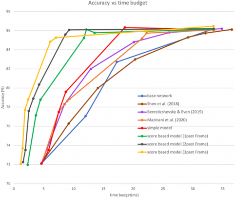
Figure 5 depicts the superiority of our score-based method over other methods. The points in this chart represent the accuracy of each model based on the time budget allotted. The blue line is the base model, which specifies the accuracy of each CNN output based on processing time.
Figure 5. Accuracy versus time budget for different models on video dataset (test set)
We change the value of the $\lambda$ parameter in Eq. (13) to obtain the accuracy of other models based on different time budgets. By reducing this parameter, the importance of processing time becomes less important than the accuracy of the results, causing the model to be trained to spend more time and achieve greater accuracy. As a result, different points will be obtained based on different time budgets.
The maximum processing time per frame is 35 milliseconds, so the frame buffer in a video that runs at 30 frames per second will never be filled. Therefore, only the External time budget determines the time budget by Eq. (5).
The brown line represents the Shen et al. [20] method. In this method, a simple and fast CNN classifier is used first, and if the result accuracy is not satisfactory, a complete and costly model called Oracle is used. For a better comparison, instead of the simple model, we used our first CNN output, which is the fastest output, and instead Oracle model, we used our last CNN output, which is the most accurate output.
The purple line shows the Berestizshevsky and Even [28] model. This model is a cascade model in which each frame is processed by the next output of the CNN if the output accuracy is less than the threshold value.
The orange line shows the Mazinani et al. [30] model. This model does not consider previous frame information, and the increase in speed is because simple images are processed with fewer layers of the CNN. In most of the given time budgets, this model outperformed the base model.
The red line shows our simple model. This model only considers previous frame information if the previous frame was processed by the deepest CNN output. When the time budget is low, the deepest output is usually not processed, so the accuracy of this model is comparable to that of the Mazinani et al. [30] model in this case. But with the increase of time budget and increasing use of the deepest CNN output, the use of the previous frame is increased and the accuracy of the simple model is much higher than the previous models so that by spending 18.6 milliseconds, its accuracy is equal to the deepest CNN output (with a time of 35 milliseconds).
Our score-based model is drawn by the green line. This model employs the scoring function to make use of any data from the previous frame. So even at much lower budgets than other models, it can produce accurate results. When the budget is very limited, and the previous frame information is reliable, the model does not process the current frame and instead uses the previous frame to specify the current frame label. As a result, in time budgets where previous models could not even produce any results (time budget less than 4.65 milliseconds), this method can produce an accurate result (up to 2X speed-up). The use of the past two and three frames is indicated by gray and yellow lines, respectively. It is clear that with the increase in the use of past frames, the processing speed has increased.
We calculated the area under the curve for the various models in Figure 5 and show it in Table 2 to thoroughly compare the models and show which model is generally superior to the others.
Table 2. The area under the curve for all models in accuracy versus time budget chart
|
Model |
Area under the curve |
Speed-up |
|
Base network |
327.7 |
1 |
|
Shen et al. [20] |
317.1 |
1.04 |
|
Berestizshevsky and Even [28] |
391 |
1.28 |
|
Mazinani et al. [30] |
386.5 |
1.5 |
|
Our simple model |
413 |
1.8 |
|
Our score-based model (1 past frame) |
629.2 |
2.75 |
|
Our score-based model (2 past frame) |
714.3 |
3.61 |
|
Our score-based model (3 past frame) |
742.7 |
4.7 |
The score-based model clearly outperforms other models in the area under the curve. In the last column of the table, we also displayed the speed-up relative to the deepest CNN output for various models. The highest accuracy of each model is used for this comparison; the difference in accuracy is less than 1 percent and negligible. According to this table, the final score-based model (3 past frames) increased the speed by 4.7 times while maintaining the final accuracy. However, this increase in speed has drawbacks, which will be discussed in the following section.
4.4 Accuracy after changing the scene content
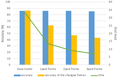
As shown in the previous section, the classification accuracy improves as more past frames are used, but the selected label becomes more dependent on the label of the previous frames. As a result, when the content of the scene changes, identifying the next frames becomes more difficult. We introduce a new criterion to detect this error in our presented models. We report the accuracy of the first two frames after changing the frame label in Figure 6. The green line represents the frame processing time for different models with an accuracy of nearly 86%. The blue columns represent total accuracy, while the yellow columns represent accuracy on the two frames after changing the scene content.
Both accuracies are close to 86% in the base model, at 33.36 milliseconds. As the use of previous frames increases, the accuracy on the first frames after a changed scene decreases. As a result, the accuracy of models that use the past two or three frames is less than 50%. So, when the label is changed, these models will almost certainly select the incorrect label for the frames. If this error is significant in an application, the best model is to use a single previous frame.
Figure 6. Accuracy on the first two frames after changing the label
4.5 Analysis of results
The results obtained in the previous section showed that due to the high semantic correlation between consecutive frames, the use of previous frame information increased the accuracy and speed of classification. For a more detailed analysis of the score-based model (1 past frame), we show the amount of one past frame usage and CNN outputs usage in Figure 7. This value is expressed as a probability and indicates the proportion of each output or past frame used.
The purple line indicates the use of the previous frame. Since the previous frame is already processed, there is no cost in using it to process the current frame, so the decision-maker module uses the previous frame's information for all given time budgets. Only when the given time is maximum, the probability of using the previous frame is close to zero. When the time budget is not limited, the decision-maker uses the maximum output power of CNN. It is also possible that the content of the frame has changed from the previous frame. Therefore, the decision-maker in the training process has concluded that using the past frame does not help to increase accuracy in this case.
Figure 7. Probability of using the previous frame and each CNN output versus the given time budget for the score-based method
The deepest and most accurate output of CNN (output 4) is marked in yellow. As the time budget has increased, so has the use of this output to improve accuracy, to the point where the probability of use is equal to one and this output is used to process all frames.
As shown in the figure, faster CNN outputs (output 1 and output 2) are used in very limited time budgets. As the given time increases, the use of slower but more accurate outputs (output 3 and output 4) becomes more. Convolution layers are common between the last outputs and the previous outputs. So, the last outputs have the information of the previous outputs as well. Therefore, if the decision-maker uses deeper outputs, it reduces the possibility of using the previous outputs.
This paper aimed to present a model that can process video frames in real-time and detect pornographic frames while also being adaptive, that is, adaptable to hardware or time constraints. For this purpose, a decision-maker with a reinforcement learning structure was designed that by simultaneously considering the accuracy and processing time, could meet both of these goals well. To extract the appropriate label for each frame of video, the decision-maker considers both the previous frame and the appropriate CNN outputs for processing in order to perform the best classification in the given time budget. Based on the results, it was found that intelligent use of the past frame can greatly increase the speed and accuracy of frame recognition.
In the future, we plan to design a decision-maker that can reprocess past frames or even check future frames. If there is enough time, the decision-maker can reprocess the previously unprocessed frame, and increase classification accuracy.
[1] Wang, L., Zhang, J., Wang, M., Tian, J., Zhuo, L. (2020). Multilevel fusion of multimodal deep features for porn streamer recognition in live video. Pattern Recognition Letters, 140: 150-157. https://doi.org/10.1016/j.patrec.2020.09.027
[2] Lykousas, N., Gomez, V., Patsakis, C. (2018). Adult content in social live streaming services: Characterizing deviant users and relationships. 2018 IEEE/ACM International Conference on Advances in Social Networks Analysis and Mining (ASONAM), Barcelona, Spain, pp. 375-382. https://doi.org/10.1109/ASONAM.2018.8508246
[3] Moustafa, M. (2015). Applying deep learning to classify pornographic images and videos. arXiv preprint arXiv:1511.08899.
[4] Wehrmann, J., Simões, G.S., Barros, R.C., Cavalcante, V.F. (2018). Adult content detection in videos with convolutional and recurrent neural networks. Neurocomputing, 272: 432-438. https://doi.org/10.1016/j.neucom.2017.07.012
[5] Yatawatte, H., Dharmaratne, A. (2015). Content based video retrieval for obscene adult content detection. Lecture Notes in Computer Science, 9492: 384-392. https://doi.org/10.1007/978-3-319-26561-2_46
[6] Kim, C.Y., Kwon, O.J., Kim, W.G., Choi, S.R. (2008). Automatic system for filtering obscene video. International Conference on Advanced Communication Technology, Gangwon, Korea (South), pp. 1435-1438. https://doi.org/10.1109/ICACT.2008.4494034
[7] Devani, U.B. Nikam, V.B., Meshram, B.B. (2014). On the fly porn video blocking using distributed multi-GPU and data mining approach. International Journal of Distributed and Parallel Systems, 5(4). https://doi.org/10.5121/ijdps.2014.5401
[8] Lohithashva, B.H., Aradhya, V.N.M., Guru, D.S. (2020). Violent video event detection based on integrated LBP and GLCM texture features. Revue d’Intelligence Artificielle, 34(2): 179-187. https://doi.org/10.18280/ria.340208
[9] Perez, M., Avila, S., Moreira, D., Moraes, D., Testoni, V., Valle, E. (2017). Video pornography detection through deep learning techniques and motion information. Neurocomputing, 230: 279-293. https://doi.org/10.1016/j.neucom.2016.12.017
[10] Yuan, C., Zhang, J. (2020). Violation detection of live video based on deep learning. Scientific Programming, 2020: 1895341. https://doi.org/10.1155/2020/1895341
[11] Mallmann, J., Santin, A.O., Viegas, E.K., dos Santos, R.R., Geremias, J. (2020). PPCensor: Architecture for real-time pornography detection in video streaming. Future Generation Computer Systems, 112: 945-955. https://doi.org/10.1016/j.future.2020.06.017
[12] Swardiana, I.W.P., Setyanto, A., Sudarmawan. (2019). Comparison of pornographic image classification based on texture, color, and shape features. 2019 4th International Conference on Information Technology, Information Systems and Electrical Engineering (ICITISEE), Yogyakarta, Indonesia, pp. 95-100. https://doi.org/10.1109/ICITISEE48480.2019.9003842
[13] Kusrini, Al Fatta, H., Pariyasto, S., Wijaya Widiyanto, W. (2019). Prototype of pornographic image detection with YCBCR and color space (RGB) methods of computer vision. 2019 International Conference on Information and Communications Technology, Yogyakarta, Indonesia, pp. 117-122. https://doi.org/10.1109/ICOIACT46704.2019.8938524
[14] Nuraisha, S., Pratama, F.I., Budianita, A., Soeleman, M.A. (2017). Implementation of K-NN based on histogram at image recognition for pornography detection. Proceedings - 2017 International Seminar on Application for Technology of Information and Communication, Semarang, Indonesia, pp. 5-10. https://doi.org/10.1109/ISEMANTIC.2017.8251834
[15] Hartatik, Setyanto, A., Kusrini, K., Agastya, I.M.A. (2019). Comparison of SIFT and SURF methods for porn image detection. 2019 4th International Conference on Information Technology, Information Systems and Electrical Engineering (ICITISEE), Yogyakarta, Indonesiap, pp. 281-285. https://doi.org/10.1109/ICITISEE48480.2019.9003773
[16] Mahadeokar, J., Pesavento, G. (2016). Open Sourcing a Deep Learning Solution for Detecting NSFW Images. Yahoo Engineering, 24, 2018.
[17] He, K., Zhang, X., Ren, S., Sun, J. (2016). Deep residual learning for image recognition. Proceedings of the IEEE Computer Society Conference on Computer Vision and Pattern Recognition, Las Vegas, NV, USA, pp. 770-778. https://doi.org/10.1109/CVPR.2016.90
[18] Deng, J., Dong, W., Socher, R., Li, L.J., Li, K., Li, F.F. (2009). Imagenet: A large-scale hierarchical image database. Computer Vision and Pattern Recognition, Miami, FL, USA, pp. 248-255. https://doi.org/10.1109/CVPR.2009.5206848
[19] Ou, X., Ling, H., Yu, H., Li, P., Zou, F., Liu, S. (2017). Adult image and video recognition by a deep multicontext network and fine-to-coarse strategy. ACM Transactions on Intelligent Systems and Technology, 8(5): 68. https://doi.org/10.1145/3057733
[20] Shen, R., Zou, F., Song, J., Yan, K., Zhou, K. (2018). EFUI: An ensemble framework using uncertain inference for pornographic image recognition. Neurocomputing, 322: 166-176. https://doi.org/10.1016/j.neucom.2018.08.080
[21] Iandola, F.N., Han, S., Moskewicz, M.W., Ashraf, K., Dally, W.J., Keutzer, K. (2016). SqueezeNet: AlexNet-level accuracy with 50x fewer parameters and <0.5MB model size. arXiv:1602.07360.
[22] Howard, A.G., Zhu, M., Chen, B., Kalenichenko, D., Wang, W., Weyand, T., Andreetto, M., Adam, H. (2017). Mobilenets: Efficient convolutional neural networks for mobile vision applications. arXiv:1704.04861.
[23] Zhang, X., Zhou, X., Lin, M., Sun, J. (2018). ShuffleNet: An extremely efficient convolutional neural network for mobile devices. 2018 IEEE/CVF Conference on Computer Vision and Pattern Recognition, Salt Lake City, UT, USA, pp. 6848-6856. https://doi.org/10.1109/CVPR.2018.00716
[24] Ma, N., Zhang, X., Zheng, H.T., Sun, J. (2018). ShuffleNet V2: Practical guidelines for efficient CNN architecture design. Lecture Notes in Computer Science (Including Subseries Lecture Notes in Artificial Intelligence and Lecture Notes in Bioinformatics), Munich, Germany, pp. 122-138. https://doi.org/10.1007/978-3-030-01264-9_8
[25] Bengio, E., Bacon, P.L., Pineau, J., Precup, D. (2015). Conditional computation in neural networks for faster models. arXiv:1511.06297.
[26] Lin, J., Rao, Y., Lu, J., Zhou, J. (2017). Runtime neural pruning. Proceedings of the 31st International Conference on Neural Information Processing Systems, Long Beach, CA, USA, pp. 2178-2188.
[27] Rao, Y., Lu, J., Lin, J., Zhou, J. (2019). Runtime network routing for efficient image classification. IEEE Transactions on Pattern Analysis and Machine Intelligence, 41: 2291-2304. https://doi.org/10.1109/TPAMI.2018.2878258
[28] Berestizshevsky, K., Even, G. (2019). Dynamically sacrificing accuracy for reduced computation: Cascaded inference based on SoftMax confidence. International Conference on Artificial Neural Networks, Munich, Germany, pp. 306-320. https://doi.org/10.1007/978-3-030-30484-3_26
[29] Bolukbasi, T., Wang, J., Dekel, O., Saligrama, V. (2017). Adaptive neural networks for efficient inference. International Conference on Machine Learning, Sydney, Australia, pp. 527-536.
[30] Mazinani, M.R., Hoseini, S.M., Dadashtabar Ahmadi, K. (2020). Time-sensitive adaptive model for adult image classification. Computing and Informatics, 39: 1282-310. https://doi.org/10.31577/cai_2020_6_1282
[31] Chatfield, K., Simonyan, K., Vedaldi, A., Zisserman, A. (2014). Return of the devil in the details: Delving deep into convolutional nets. Proceedings of the British Machine Vision Conference 2014, British Machine Vision Association. https://doi.org/10.5244/C.28.6
[32] Watkins, C.J.C.H., Dayan, P. (1992). Q-learning. Machine Learning, 8: 279-292. https://doi.org/10.1007/BF00992698
[33] Mirhashemi, M.H., Anvari, R., Barari, M., Mozayani, N. (2020). Test-cost sensitive ensemble of classifiers using reinforcement learning. Revue d’Intelligence Artificielle, 34(2): 143-150. https://doi.org/10.18280/ria.340204
[34] Noktedan, A. (2020). Adult content dataset. https://doi.org/10.6084/m9.figshare.13456484.v1