Pratibha Verma* | Vineet Kumar Awasthi | Sanat Kumar Sahu
© 2021 IIETA. This article is published by IIETA and is licensed under the CC BY 4.0 license (http://creativecommons.org/licenses/by/4.0/).
OPEN ACCESS
Data mining techniques are included with Ensemble learning and deep learning for the classification. The methods used for classification are, Single C5.0 Tree (C5.0), Classification and Regression Tree (CART), kernel-based Support Vector Machine (SVM) with linear kernel, ensemble (CART, SVM, C5.0), Neural Network-based Fit single-hidden-layer neural network (NN), Neural Networks with Principal Component Analysis (PCA-NN), deep learning-based H2OBinomialModel-Deeplearning (HBM-DNN) and Enhanced H2OBinomialModel-Deeplearning (EHBM-DNN). In this study, experiments were conducted on pre-processed datasets using R programming and 10-fold cross-validation technique. The findings show that the ensemble model (CART, SVM and C5.0) and EHBM-DNN are more accurate for classification, compared with other methods.
coronary artery disease, deep learning, neural network, support vector machine, ensemble model
Coronary Artery Disease (CAD) is a common but serious disease and is the main cause of the heart attack in humans. Common people ignore the initial symptoms and signs of CAD problems due to economic limitations. This causes economic and psychological effects in their lives [1]. Studies have been conducted to diagnose CAD at early stages in a way that is economically viable for the common man. The data mining techniques are included with ensemble learning and deep learning for the classification of the CAD. Various healthcare and medical science organizations, as a matter of routine and clinical check-up, capture huge amount of historical data, which describe the patients’ health condition, disease and disease diagnosis routine. At the same time, researchers and scientists in various fields capture datasets that are increasing in terms of complexity. Data mining is a technique to find the hidden pattern from the historical data and enhance the decision-making process [2]. A decision tree can be called a map of the reasoning process. It is a hierarchical set of rules which explain that how to classify a large dataset into smaller dataset partitions. All time a partition occurs, the resulting division's components move correspondingly regarding concerning the target [3, 4].
In this study, we have used two decision trees namely Single C5.0 Tree (C5.0) and Classification and Regression tree (CART). The Support Vector Machine (SVM) utilizes a method called the kernel trick to transform the data. Based on these transformations it finds an optimal boundary between the possible outputs [5]. We have used the kernel-based Support Vector Machine with the linear kernel (SVM). The ensemble model combines a set of classifiers to produce a single compound model that offers higher accuracy [6, 7]. Stacking, also referred to as a stacked generalization or meta ensemble model, is a new well-known technique that is used to reduce the generalization error rate by reducing the bias of generalizers [8]. In this study, an ensemble model combination of three classifiers namely C5.0, CART, SVM has been used. The Artificial Neural Network (ANN) is a new dimension for different types of research purposes. The ANN has been developed based on the human brain’s internal working architecture and processing system [9]. Two different variants of ANN namely Neural Network (NN) and Neural Network with feature Extraction (PCA-NN) have been used in this study. Another ANN-based learning dimension in the recent days i.e., Deep Learning Network (DL) or Deep Neural Network (DNN) is very popular. It is an ANN learning with increased number of the hidden layers in the internal architecture and enhanced computational speed of the learning algorithm [10, 11]. In this research, DNN based H2OBinomialModel-Deeplearning (HBM-DNN) and Enhanced H2OBinomialModel-Deeplearning (EHBM-DNN) have been used. Finally, we compared the proposed model's classification accuracy, sensitivity, specificity and F1-Score with other classifiers. The proposed ensemble (CART, SVM, C5.0) and EHBM-DNN models assist in a quick identification and early detection of CAD.
Several studies have been conducted to demonstrate the utility of data mining models in CAD-related problems.
Polat and Gunes [12] worked on fuzzy weighted pre-processing, used the classifier AIRS and achieved an accuracy of 92.59% for diagnosing CAD, compared with Rajkumar and Reena [13] who used KNN, Naïve Bayes (NB) and decision tree Techniques and obtained the highest accuracy of 52.33% with NB. Swain et al. [14] proposed a Dense Neural Network for classification of the Cleveland Heart disease data. They obtained a classification accuracy of 94.91% during testing, whereas 83.67% of accuracy was achieved by Miao, K.H. and Miao, J.H. [15] by using the enhanced Deep Neural Network (DNN) learning with regularization and dropout model for heart disease diagnosis. Bektas et al. [16] worked on the cardiovascular dataset with various methods like Logistic regression RNA, NN, FST like Relief-F and Independent t-test analysis. The outcomes show that 84.1% NN accuracy was obtained with the oversampled dataset and the Relief-f feature selection method. El-Bialy et al. [17] worked on fast Decision Tree and prune C 4.5 tree. The outcome showed that the classification performance of the collected datasets was 78.06% and that it was better than different datasets. Alizadehsani et al. [18] worked on the SMO, Naïve Bayes and ensemble algorithms for investigation. The ensemble algorithm obtained 88.5% accuracy. Alizadehsani et al. [19] employed the algorithms KNN, SVM, SMO, Naive Bayes and C4.5 in the CAD dataset. The outcome showed that the SMO obtained a high accuracy of 92.09%.
Data mining and machine learning have been proved to be effective in modelling medical science and healthcare like Coronary Artery Disease (CAD). In this study, for modelling of CAD, we used the classification algorithms based on: decision treeC5.0 and CART, linear kernel SVM, Neural Network Fit single-hidden-layer neural network (NN) and Neural Networks with Feature Extraction (PCA-NN), deep learning H2OBinomialModel-Deeplearning (two hidden layers and Five Neurons in each hidden layer) (HBM-DNN) and Enhanced H2OBinomialModel-Deeplearning (three hidden layers and Twenty Neurons in each hidden layer) (EHBM-DNN)and ensemble learning-based ensemble(CART, SVM, C5.0). The schematic of the methodology of this research is presented in Figure 1.
Figure 1 shows the schematic of the methodology of data mining and machine learning technology used in this research work. A lot of classification techniques have been developed for disease detection. This technique offers high accuracy in the detection of disease.
3.1 Data collection and analysis
The experimental data sets used are Z-Alizadeh Sani and extension Z-Alizadeh Sani available on the UC Irvine Machine Learning Repository. The two data sets hold the records of 303 patients each of which has 54 features (attributes) and 59 features (attributes) [20, 21] respectively.
3.2 Pre-processing of data
The purpose of data pre-processing techniques is to eliminate inconsistency from the dataset and improve data quality, especially in the case of a data mining-based classification analysis models for smooth convergence of learning models. It implemented the following pre-processing techniques:
Correlation coefficient
The correlation coefficient is a measure of the strength and the direction of a linear relationship between two variables [22]. The default is the Pearson correlation coefficient which measures the linear dependence between two variables. It is defined as follows. Suppose there are two variables X and Y, each having n values X1, X2, …, Xn and Y1, Y2, …, Yn respectively. Let the mean of X be $\bar{X}$ and the mean of Y be $\bar{Y}$. The Pearson correlation coefficient r in given by Eq. (1).
$\mathbf{r}=\frac{n \sum x y-\left(\sum x\right)\left(\sum y\right)}{\sqrt{n \sum x^{2}-\left(\sum x\right)^{2}} \sqrt{n \sum y^{2}-\left(\sum y\right)^{2}}}$ (1)
The range of the correlation coefficient is -1 to 1. If x and y have a strong positive linear correlation, r is close to 1. If x and y have a strong negative linear correlation, r is close to -1. If there is no linear correlation or a weak linear correlation, r is close to 0.
Figure 1. Schematic view of proposed methodology
3.3 Data mining and machine learning methods
Today various data sources, as a matter of routine, capture a massive amount of historical data, which describe operation, nature and behaviour. At the same time, researchers and scientists in various fields capture datasets that are growing in terms of complexity. Data mining arrives at the best way of using historical data to find the pattern and improve the decision-making process. The set of techniques for extracting (predictive) models from the data constitutes the field of machine learning [3].
CART
Classification and Regression Trees (CART) was proposed by Breiman et al. [23]. It also reflects the greedy, top-down and divide-and-conquer methods for the construction of the binary decision tree. This tree may be used for classification and regression purposes. The Gini index is used as the splitting parameter to define an attribute to be considered for a node. The Gini index measures impurity in the data using Eq. (2).
$\operatorname{Gini}(d)=1-\sum_{j=1}^{m} p^{2} \mathrm{j}$ (2)
where, pj is the probability that a sample belongs to the class Cj. pjis computed using|Ci,D|/|D|, i.e., the ratio between the number of samples of class I and the total number of samples of the dataset.
C5.0
C5.0 is another new decision tree algorithm based on C4.5 by Quinlan [24]. C4.5 in turn has evolved based on ID3. The idea of building a decision tree in C5.0 is similar to C4.5. C5.0 introduces more new technologies, including all the functions of C4.5. One of the important technologies is boosting and another is the construction of a cost-sensitive tree [25]. Fit classification tree model or rule-based model uses Quinlan's C5.0 algorithm. The model can take the form of a complete decision tree or a collection of rules. When using the formula method, factors and other classes are preserved. The classification task using C5.0 with the number of tuning parameters and boosting iterations [26].
Support vector machine
The support vector machine is a supervised learning method used for non-linear complex tasks. It can be used for classification or regression work. A model is built using the SVM training algorithm that provides new samples to one class or the other based on the training set. Kernels in SVM are used to check for similarities between instances. The formation of the resulting classifier is now generalized enough and can be used for the classification of new samples [5, 27].
For nonlinear transformation, the input variable in the SVM algorithm is transformed into a high-dimensional linear feature space. Therefore the optimum decision function is built [28]. Then the dot product operation in the high dimensional feature space is converted using the kernel function stored in the original space and the classification function is determined according to the equation,
f(x)=ωT.Φ(x)+b (3)
where, ω defines the weight vector, B represents the bias term and Φ(x)is the nonlinear transformation function.
Neural Network (NN)
Fit single-hidden-layer neural network, possibly with skip-layer connections. The MLP networks may have special connections called the Skip Layer. In this, the input signals (layer) have a direct connection to the output layer, i.e., implementing the hidden layer [9, 29]. The Figure 2 shows the fit single hidden layer neural network.
Figure 2. Fit single-hidden-layer neural network
The signal is received from the nodes of the input layer, by the hidden layer, wherein each input variable is multiplied by a respective weight and its sum is added to bias [9].
Output function:
yk=bk+x0w0+x1w1+x2w2 (4)
where, x0,x2,x3 are input signals and w0,w1,w2 are synaptic weights and bk is bias signal.
Principal Component Analysis with Neural Network (PCA-NN)
The PCA-NN first computes the Principal Components Analysis (PCA) of the dataset and the cumulative parentage of the variance for every principal component. The function uses a logic statement to estimate how many components must be preserved in the predictors to absorb the number of variants. Essentially, the classical PCA aims to solve an eigenvalue problem:
Cxaj = λjaj, for j = 1, 2, ..., p (5)
where, Cx is the original data covariance matrix, λj is an eigenvalue of Cx and aj is the eigenvector corresponding to the eigenvalue λj. Next, the calculated eigenvalues can be increasingly ordered:
λ1 ≥λ2 ≥…. λp (6)
The principal components can, then, be computed according to the equation:
Zj = aTj X = XT aj, for j = 1, 2, ...,p (7)
where, Zj is the j-th principal component and X represents the original data set. An important property of PCA is that the variances of principal components are the eigenvalues of matrix C. Therefore, dimensionality reduction can be obtained by performing PCA and by keeping only the components with highest variance PCA needed 45 components to capture 95 percent of the variance in Alizadeh Sani. PCA needed 47 components to capture 95 percent of the variance in Extension of Alizadeh Sani. The PCA-Neural Network uses an unsupervised learning process that is based on variations of the Neural Network rule [30].
H2OBinomial-Model-Deep Neural Network (HBM-DNN)
The DNN Classifier was built using H2O package of R Programming for training and modelling. It is using open source, in-memory, scalable machine learning and AI platform used to create models with large dataset and implement classification with high accuracy methods [11]. The H2OBinomial-Model-Deep Learning or H2OBinomial-Model-Deep Neural Network (HBM-DNN) involves building a feed-forward multilayer artificial neural network on aH2OFrame. H2O's Deep Learning calculation has been fundamentally utilized for building the models. The Deep Learning calculation depends on a multi-layer feed-forward fake neural organization that is prepared with stochastic inclination plunge utilizing back-spread. The shrouded contentions are utilized to set the quantity of concealed layers and neurons for each shrouded layer.
Our HBM-DNN contains 56 units in the Input layer, 5, 5, 5 neurons in every one of the 2 concealed layers separately and 2 neurons in yield layers. This HBM-DNN is ordered the Z-Alizadeh Sani and expansion of Z-Alizadeh Sani (CAD) datasets. In our investigation, we have utilized a DNN called the HBM-DNN with two concealed layers and five neurons for each shrouded layer. We likewise propose the Enhanced H2OBinomial-Model-Deep Neural Network (EHBM-DNN) with three shrouded layers and twenty neurons for each concealed layer.
The Figure 3 represent the architecture of our proposed EHBM-DNN contains 56 units in the Input layer, 20, 20, 20 neurons in each of the 3 hidden layers and Figure 4 shows the architecture 59 units in the Input layer, 20, 20, 20 neurons in each of the 3 hidden layers with two neurons in output layers respectively.
Ensemble techniques
An ensemble learning technique combines multiple classifiers and gives the final prediction (classification results). The ensemble model combines a set of classifiers to produce a single compound model that offers higher accuracy. Ensemble methods can be termed as the committee, classifier fusion, combination or aggregation, etc. Ensemble methods can be classified as Homogeneous Ensemble [31] Methods and Heterogeneous ensemble [32] methods. Homogeneous ensemble Methods use a single learning algorithm on different training datasets to construct multiple classifiers such as Bagging, Boosting, Random Subspaces, Random Forest, etc. Heterogeneous ensemble methods use a variety of learning algorithms and manipulate the training datasets to make multiple models. Some of the heterogeneous methods are voting, stacking, etc.
Stacking, also referred to as a stacked generalization or meta ensemble model, is a new well-known technique that is used to reduce the generalization error rate by reducing the bias of generalizers. Stacking introduces the concept of a Meta-learner, which replaces the voting procedure [33]. The problem with voting is that it is not clear which classifier to trust. Stacking tries to learn which classifiers are the reliable ones, using another learning algorithm—the Meta-learner—to discover how best to combine the output of the base learners. It merges the output of several classification models (level-0 base model) as training data for another model (level-1 stacked model) to estimate the same target function. The second level model learns where each base learner performs better, thus achieving better classification accuracy [34]. In this study, we can easily specify the base classifiers, the meta-learner and the number of cross-validation folds.
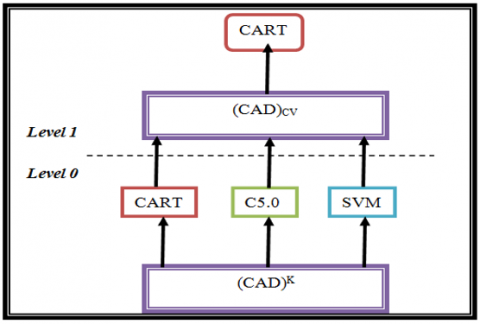
Figure 5 shows the k-fold cross-validation method in Level-0, and the level-1 used datasets (CAD)CV at the end of this method are used to produce level-1 model CART. We used three classification algorithms we used for the stack generalization process. In this level-1 or meta-classifier is CART, level-0 or base learners are CART, C5.0, and SVM.
Figure 5. Schematic view of stacked ensmble model
Performance evaluation
We calculated the performance of classifiers based on the following confusion matrix are shown in Table 1.
Table 1. Confusion matrix
|
Actual Vs. Predicted |
Positive |
Negative |
|
Positive |
True Positive (TP) |
False Negative (FN) |
|
Negative |
False Positive (FP) |
True Negative (TN) |
The performance of the classification models was measured using four performance measures: accuracy, sensitivity, specificity and f-measure. Accuracy is the percentage of correctly classified instances among all instances. Sensitivity analysis techniques measure the rate of change at the output of a sample due to adjustments in the input of a variable. Specificity analysis is the proportion of actual negatives that are correctly identified. F-measure is the harmonic mean of Precision and Recall and gives a better measure of the incorrectly classified cases than the Accuracy Metric.
Accuracy $=\frac{T P+T N}{T P+T N+F P+F N}$ (8)
Sensitivity $=\frac{T P}{T P+F N}$ (9)
Specificity $=\frac{T N}{T N+F P}$ (10)
F1-Score $=\frac{2 T P}{(2 T P+F P+F N)}$ (11)
In this study, we used the R software and its different packages and methods for data analysis. For a comparative study of the classification models, the performances of the proposed classification models are shown in Table 2.
Table 2. Performance of classifiers (in %)
|
Z-Alizadeh Sani dataset |
||||
|
Algorithm |
Accuracy |
Sensitivity |
Specificity |
F1-Score |
|
CART |
83.19 |
89.33 |
67.91 |
88.30 |
|
SVM |
78.55 |
92.55 |
43.75 |
86.11 |
|
Single C5.0 Tree |
82.24 |
89.76 |
63.75 |
87.77 |
|
Ensemble (CART+SVM+C5.0) |
83.47 |
92.12 |
62.08 |
88.88 |
|
NN |
71.95 |
83.23 |
97.72 |
83.23 |
|
PCA-NN |
83.12 |
87.38 |
72.36 |
87.93 |
|
HBM-DNN |
82.51 |
80.1 |
88.51 |
86.72 |
|
EHBM–DNN |
96.04 |
95.83 |
96.55 |
97.18 |
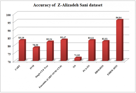
Table 2 presents a comparison of results using the Z-Alizadeh Sani CAD dataset. It gives a comparison of the results obtained from the classifiers CART, SVM, Single C5.0 Tree, Ensemble (CART + SVM + C5.0), NN, PCA-NN, HBM-DNN and EHBM-DNN. The highest accuracy of 96.04% is obtained by the proposed EHBM–DNN model compared with other models. The accuracy of the proposed ensemble (CART + SVM + C5.0) 83.47% is the second-highest accuracy of all the models. Sensitivity analysis techniques measure the rate of change at the output of a sample due to adjustments in the input of a variable. The maximum sensitivity of 95.84% is obtained by the proposed EHBM–DNN model compared with other models. Specificity analysis is the proportion of actual negatives that are correctly identified. The maximum specificity of 97.72% is obtained by the proposed NN model compared with other models. The F1-Score is the harmonic mean of Precision and Recall and gives a better measure of the incorrectly classified cases than the accuracy metric. Among all classifier models, the maximumF1-Scoreof 94.31% is obtained by the proposed EHBM–DNN model. The F1-Score of the ensemble (CART + SVM + C5.0) is 88.88%.
Figure 6. Accuracy comparison of Z-Alizadeh Sani dataset
In Figure 6, the accuracy results for the Z-Alizadeh Sani dataset are shown for various proposed models. The classification performance computed in Accuracy measured is the True Positives and True negatives are more significant. The chart demonstrates the best and worst outcomes from all the models.
For a comparative study of the classification models, the performances of the proposed classification models are shown in Table 3.
Table 3. Performance of classifiers (in %)
|
Extension of Z-Alizadeh Sani dataset |
||||
|
Algorithm |
Accuracy |
Sensitivity |
Specificity |
F1-Score |
|
CART |
96.34 |
95.32 |
98.88 |
97.27 |
|
SVM |
85.50 |
89.41 |
75.83 |
89.69 |
|
Single C5.0 Tree |
99.67 |
99.77 |
100 |
98.88 |
|
Ensemble (CART+SVM+C5.0) |
99.67 |
99.77 |
100 |
98.88 |
|
NN |
78.71 |
94.91 |
39.58 |
86.67 |
|
PCA-NN |
96.04 |
94.93 |
98.89 |
97.11 |
|
HBM-DNN |
87.79 |
87.50 |
88.51 |
91.09 |
|
EHBM–DNN |
99.67 |
99.54 |
100 |
99.76 |
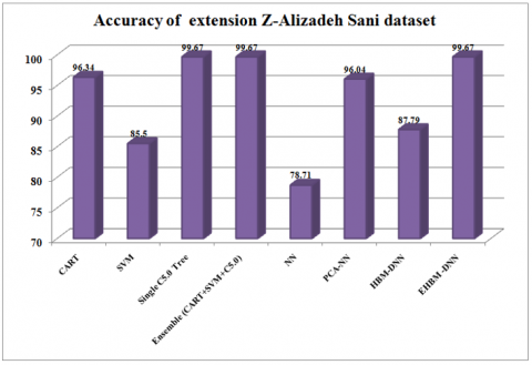
Table 3 presents a comparison of results using the extension of the Z-Alizadeh Sani CAD dataset. The classifiers Single C5.0 Tree, Ensemble (CART + SVM + C5.0) and EHBM-DNN obtained the maximum accuracy of 99.67% compared to other models. Sensitivity analysis techniques measure the rate of change at the output of a sample due to adjustments in the input of a variable. The maximum sensitivity of 99.77% is obtained by the proposed Single C5.0 Tree and Ensemble (CART + SVM + C5.0) models compared with other models. Specificity analysis is the proportion of actual negatives that are correctly identified. The maximum specificity of 100% is obtained by the proposed Single C5.0 Tree, Ensemble (CART + SVM + C5.0) and EHBM-DNN models compared to other models. The F1-Score is the harmonic mean of Precision and Recall and gives a better measure of the incorrectly classified cases than the accuracy metric. The maximumF1-Scoreof 99.76% is obtained by the proposed EHBM–DNN model compared to other models. TheF1-Score of the ensemble (CART + SVM + C5.0) is 98.88%.
Figure 7 shows the accuracy results for the extension Z-Alizadeh Sani dataset for various proposed models. The classification performance computed in accuracy measured is the true positives and true negatives are more significant. The chart demonstrates the best and worst outcomes from all the models.
Figure 7. Accuracy comparison of extension Z-Alizadeh Sani dataset
This study applied CAD datasets to eight classification methods CART, C5.0, SVM, ensemble (CART, SVM, C5.0), NN, PCA-NN, HBM-DNN and EHBM-DNN. The performance of all the algorithms were compared with respect to accuracy, sensitivity, specificity and F1-Score. The findings demonstrate that, of all the cases in the CAD dataset, the proposed ensemble (CART, SVM, C5.0) and EHBM-DNN performed efficiently and accurately. The EHBM-DNN and the ensemble model in the extension of the Z-Alizadeh Sani data set obtained the optimum accuracy of 99.67%. The EHBM-DNN in the Z-Alizadeh Sani dataset achieved the highest accuracy of 96.04%.
Finally, the experimental findings show that the proposed EHBM-DNN and ensemble model outperform existing method in terms of performance and hence it is best suitable for contrast enhancement of CAD dataset classifications. Other deep learning and data mining techniques might be applied in the future to improve the outcomes.
[1] Alizadehsani, R., Habibi, J., Hosseini, M.J., Boghrati, R. (2012). Diagnosis of coronary artery disease using data mining techniques based on symptoms and ECG features. European Journal of Scientific Research, 82(4): 542-553.
[2] Alizadehsani, R., Habibi, J., Hosseini, M.J., Mashayekhi, H., Boghrati, R., Ghandeharioun, A., Sani, Z.A. (2013). A data mining approach for diagnosis of coronary artery disease. Computer Methods and Programs in Biomedicine, 111(1): 52-61. https://doi.org/10.1016/j.cmpb.2013.03.004
[3] Gopal, M. (2018). Applied Machine Learning (First). Delhi: Mc Graw Hill Education.
[4] Han, J., Kamber, M., Pei, J. (2012). Data Mining: Concepts and Techniques (third). Elsevier. https://doi.org/10.1016/C2009-0-61819-5
[5] Cortes, C., Vapnik, V. (1995). Support-vector networks. Machine Learning, 20(3): 273-297. https://doi.org/10.1007/BF00994018
[6] Gandhi, I., Pandey, M. (2015). Hybrid ensemble of classifiers using voting. International Conference on Green Computing and Internet of Things (I CGCloT), pp. 399-404. https://doi.org/10.1109/ICGCIoT.2015.7380496
[7] Pandey, M., Taruna, S. (2014). A comparative study of ensemble methods for students' performance modeling. International Journal of Computer Applications, 103(8). https://doi.org/10.5120/18095-9151
[8] Wolpert, D.H. (1992). Stacked generalization. Neural Networks, 5(2): 241-259. https://doi.org/10.1016/S0893-6080(05)80023-1
[9] Haykin, S. (2008b). Neural Networks and Learning Machines. Pearson Prentice Hall New Jersey USA 936 pLinks (Vol. 3).
[10] Bengio, Y., Courville, A., Vincent, P. (2013). Representation learning: A review and new perspectives. IEEE Transactions on Pattern Analysis and Machine Intelligence, 35(8): 1798-1828. https://doi.org/10.1109/TPAMI.2013.50
[11] Ciaburro, G., Venkateswaran, B. (2017). Neural Network with R (first). Birmingham-Mumbai: Packt Publishing Ltd.
[12] Polat, K., Gunes, S. (2007). A hybrid approach to medical decision support systems: Combining feature selection, fuzzy weighted pre-processing and AIRS. Computer Methods and Programs in Biomedicine, 8: 164-174. https://doi.org/10.1016/j.cmpb.2007.07.013
[13] Rajkumar, A., Reena, G.S. (2010). Diagnosis of heart disease using datamining algorithm. Global Journal of Computer Science and Technology, 10(10): 38-43.
[14] Swain, D., Pani, S.K., Swain, D. (2019). An efficient system for the prediction of coronary artery disease using dense neural network with hyper parameter tuning. International Journal of Innovative Technology and Exploring Engineering (IJITEE), 8(6): 689-695.
[15] Miao, K.H., Miao, J.H. (2018). Coronary heart disease diagnosis using deep neural networks. (IJACSA) International Journal of Advanced Computer Science and Applications, 9(10): 1-8.
[16] Bektas, J., Ibrikci, T., Ozcan, I.T. (2017). Classification of real imbalanced cardiovascular data using feature selection and sampling methods: A case study with neural networks and logistic regression. International Journal on Artificial Intelligence Tools, 26(6): 1750019. https://doi.org/10.1142/S0218213017500191
[17] El-Bialy, R., Salamay, M.A., Karam, O.H., Khalifa, M.E. (2015). Feature analysis of coronary artery heart disease data sets. Procedia Computer Science, 65: 459-468. https://doi.org/10.1016/j.procs.2015.09.132
[18] Alizadehsani, R., Hosseini, M.J., Boghrati, R., Ghandeharioun, A., Khozeimeh, F., Sani, Z.A. (2012). Exerting cost-sensitive and feature creation algorithms for coronary artery disease diagnosis. International Journal of Knowledge Discovery in Bioinformatics (IJKDB), 3(1): 59-79. https://doi.org/10.4018/jkdb.2012010104
[19] Alizadehsani, R., Hosseini, M.J., Boghrati, R., Ghandeharioun, A., Khozeimeh, F., Sani, Z.A. (2012). Exerting cost-sensitive and feature creation algorithms for coronary artery disease diagnosis. International Journal of Knowledge Discovery in Bioinformatics (IJKDB), 3(1): 59-79. https://doi.org/10.4018/jkdb.2012010104
[20] Sani, Z.A., Alizadehsani, R., Roshanzami, M. (2017). Z-Alizadeh Sani Data Set. UC Irvine Machine Learning Repository. Retrieved from https://archive.ics.uci.edu/ml/datasets/extention+of+Z-Alizadeh+sani+dataset, accessed on 23 Nov. 2020.
[21] Z-Alizadeh Sani dataset. (2016). Retrieved from https://archive.ics.uci.edu/ml/datasets/extention+of+Z-Alizadeh+sani+dataset
[22] Gogtay, N.J., Thatte, U.M. (2017). Principles of correlation analysis. Journal of The Association of Physicians of India, 65(3): 78-81.
[23] Breiman, L., Friedman J.H., Olshen R.A., Stone, C.J. (1987). Classification and Regression Tree. Wadsworth and brooks Cole advanced books and software.
[24] Quinlan, J.R. (1993). C4.5: Programs for Machine Learning. San Mateo, CA: Morgan Kaufmann.
[25] Pang, S.L., Gong, J.Z. (2009). C5.0 classification algorithm and application on individual credit evaluation of banks. Systems Engineering-Theory & Practice, 29(12): 94-104. https://doi.org/10.1016/S1874-8651(10)60092-0
[26] Max, K., Weston, S., Culp, M. (2020). Package ‘C50.’ https://cran.r-project.org/web/packages/C50/C50.pdf.
[27] Silva, J., Romero, J., Patricia, A., Castillo, P., Silva, J., Romero, J., Varela, N. (2019). Integration of data mining classification techniques and integration ensemble learning for predicting the export potential of a company. Procedia Computer Science, 151(2018): 1194-1200. https://doi.org/10.1016/j.procs.2019.04.171
[28] Abdar, M., Makarenkov, V. (2019). CWV-BANN-SVM ensemble learning classifier for an accurate diagnosis of breast cancer. Measurement, 146: 557-570. https://doi.org/10.1016/j.measurement.2019.05.022
[29] Ripley, B.D. (1996). Pattern Recognition and Neural Networks. Cambridge: Cambridge University Press. https://doi.org/https://doi.org/10.1017/CBO9780511812651
[30] Oliveira, P.R., Digiampietri, L.A., Honda, W.Y., Pereira, M.C. (2016). A parallel PCA neural network approach for feature extraction. X Congresso Brasileiro de Inteligencia Computacional (CBIC’2011), pp. 1-6. https://doi.org/10.21528/cbic2011-39.6
[31] Breiman, L. (1996). Bagging predictors. Machine Learning, 24(2): 123-140. https://doi.org/10.1023/A:1018054314350
[32] Dietterich, T.G. (2000). Ensemble methods in machine learning. In: Multiple Classifier Systems. MCS 2000. Lecture Notes in Computer Science, vol 1857. Springer, Berlin, Heidelberg. https://doi.org/10.1007/3-540-45014-9_1
[33] Witten, I.H., Frank, E. (2002). Data mining: Practical machine learning tools and techniques with Java implementations. Acm Sigmod Record, 31(1): 76-77.
[34] Ting, K.M., Witten, I.H. (1999). Issues in stacked generalization. Journal of Artificial Intelligence Research, 10(1): 271-289.