Sai Sudha Sonali Palakodati | Venkata RamiReddy Chirra* | Yakobu Dasari | Suneetha Bulla
© 2020 IIETA. This article is published by IIETA and is licensed under the CC BY 4.0 license (http://creativecommons.org/licenses/by/4.0/).
OPEN ACCESS
Detecting the rotten fruits become significant in the agricultural industry. Usually, the classification of fresh and rotten fruits is carried by humans is not effectual for the fruit farmers. Human beings will become tired after doing the same task multiple times, but machines do not. Thus, the project proposes an approach to reduce human efforts, reduce the cost and time for production by identifying the defects in the fruits in the agricultural industry. If we do not detect those defects, those defected fruits may contaminate good fruits. Hence, we proposed a model to avoid the spread of rottenness. The proposed model classifies the fresh fruits and rotten fruits from the input fruit images. In this work, we have used three types of fruits, such as apple, banana, and oranges. A Convolutional Neural Network (CNN) is used for extracting the features from input fruit images, and Softmax is used to classify the images into fresh and rotten fruits. The performance of the proposed model is evaluated on a dataset that is downloaded from Kaggle and produces an accuracy of 97.82%. The results showed that the proposed CNN model can effectively classify the fresh fruits and rotten fruits. In the proposed work, we inspected the transfer learning methods in the classification of fresh and rotten fruits. The performance of the proposed CNN model outperforms the transfer learning models and the state of art methods.
agricultural industry, CNN, pre-trained models, Softmax
The recent approaches in computer vision, especially in the fields of machine learning and deep learning have improved the efficiency of image classification tasks [1-6]. Detection of defected fruits and the classification of fresh and rotten fruits represent one of the major challenges in the agricultural fields. Rotten fruits may cause damage to the other fresh fruits if not classified properly and can also affect productivity. Traditionally this classification is done by men, which was labor-intensive, time taking, and not efficient procedure. Additionally, it increases the cost of production also. Hence, we need an automated system which can reduce the efforts of humans, increase production, to reduce the cost of production and time of production.The recent approaches in computer vision, especially in the fields of machine learning and deep learning have improved the efficiency of image classification tasks [1-6]. Detection of defected fruits and the classification of fresh and rotten fruits represent one of the major challenges in the agricultural fields. Rotten fruits may cause damage to the other fresh fruits if not classified properly and can also affect productivity. Traditionally this classification is done by men, which was labor-intensive, time taking, and not efficient procedure. Additionally, it increases the cost of production also. Hence, we need an automated system which can reduce the efforts of humans, increase production, to reduce the cost of production and time of production.
A machine vision system was developed for the detection of fruit skin defects in the study [7]. Colour is the major feature used for categorization and a machine learning algorithm called Support Vector Machine (SVM) has been used in classification. Support Vector Machine (SVM) produces adequate results on a small number of datasets. The accuracy in classification using machine learning mostly based on the features drawn out and features that are chosen for passing on to the machine learning algorithm. We can improve performance by using deep learning models. These models help in the classification of images in large datasets.
Image processing [8] can help in the classification of the defect and non-defect fruits. It helps in identifying the defects on the surface of mango fruits. First, the fruits are collected manually and the researchers themselves classified them as fine and defected. Then pre-processing is carried out on the images and is given to a CNN model for the task of classification. This model produced an accuracy of 97.5%. The method based on laser backscattering imaging analysis and CNN theory provides an idea and theoretical basis for efficient, non-destructive, and online detection of fruit quality. This work shows that the method is effective and can non-destructively and automatically identify the defect regions, normal regions, stem regions, and calyx regions of apples, and the overall recognition rate is over 90%. The method can meet the requirements of the detection of apple defects, especially when the defect regions are similar to the stem and calyx regions in gray characteristics and shapes. The effect of defect recognition based on the CNN model is better than the conventional algorithms [9]. Nowadays, deep learning models with CNN are widely used in the classification of images in different problems that arise in the field of agriculture [10].
In our work, the proposed CNN model provides high accuracy in the classification task of fresh and rotten fruits. Here the proposed model’s accuracy is compared against the transfer learning models. Three types of fruits are selected from various types of fruits. The dataset is obtained from Kaggle with 6 classes i.e. each fruit is divided as fresh and rotten. We inspected the different pre-trained models of VGG16, VGG19, MobileNet, and Xception of transfer learning (transfer learning models). This paper introduces a powerful CNN model which has enhanced accuracy for fresh and rotten fruits classification task than transfer learning models while investigating the effect of very important hyperparameters to obtain better results and also avoid over-fitting.
3.1 Dataset acquisition and pre-processing
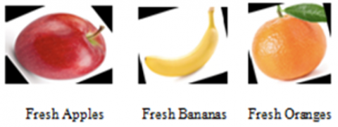
The dataset is obtained from Kaggle which has three types of fruits-apples, bananas, and oranges with 6 classes i.e. each fruit divided as fresh and rotten. The total size of the dataset used in this work is 5989 images. The training images are of 3596, the validation set contains 596 images belongs to 6 classes, and the test set contains of 1797 images which belong to 6 classes. The samples for each class in the dataset are shown Figure 1. Now the entire dataset of images is reshaped to 224x224x3 and converted into numpy array for faster convolution in case of building the CNN model. Finally, the converted dataset of images is labeled according to each class they belong. Whereas, when training the dataset using transfer learning the image augmentation is applied, validation is done in parallel while training and tested upon the test set.
Figure 1. Sample images of dataset
3.2 Convolutional neural networks
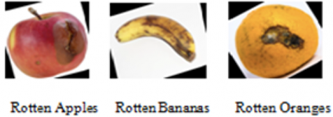
Deep Learning is a very famous division in machine learning. It shows a great level of performance across different types of data. We can use a deep learning model for building an image classification network using a convolutional neural network (CNN). The basic structure of CNN is shown in Figure 2. In computers, the images are represented as related pixels. In the image, a certain collection of pixels may represent an edge in one image, some may represent the shadow of an image or some other pattern. One way to detect these patterns is by using convolution. During computation, the image pixels are represented using a matrix. For detecting the patterns, we need to use a “filter” matrix which is multiplied with the image pixel matrix. These filter sizes may vary and the multiplication purely depends on the filter size and one can take a subset from the image pixel matrix based on the filter size for convolution starting from the first pixel in the image pixel matrix. Then the convolution moves on to the next pixel and this process is repeated until all the image pixels in the matrix are completed. While convolving, several parameters are shared. The output of a convolution is a feature map that is forwarded to the next layer.
The next type of layer used in the CNN model is the pooling layer. This layer decreases the size of the output i.e. feature map and thus avoid overfitting. The final layer used is a fully connected. This layer “flattens” the output obtained from previous layers and converts them into a single vector, which can be an input for the next state. Batch Normalizations can be used to normalize the feature maps obtained at each stage. Dropouts are also used to increase the computation speed.
Figure 2. Basic CNN architecture for classification
3.3 Proposed model for classification of fresh and rotten fruits
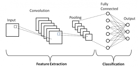
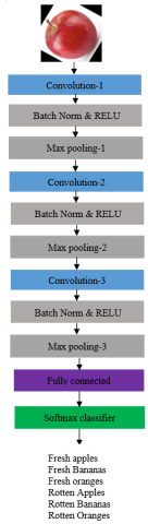
In our work, we proposed an accurate CNN model for classifying the fresh and rotten fruits which is shown in Fig 3. It consists of three convolutional layers. The first convolution layer uses 16 convolution filters with a filter size of 3x3, kernel regularizer, and bias regularizer of 0.05. It also uses random_uniform, which is a kernel initializer. It is used to initialize the neural network with some weights and then update them to better values for every iteration. Random_uniform is an initializer that generates tensors with a uniform distribution. Its minimum value is -0.05 and the maximum value of 0.05. Regularizer is used to add penalties on the layer while optimizing. These penalties are used in the loss function in which the network optimizes. No padding is used so the input and output tensors are of the same shape. The input image size is 224x224x3. Then before giving output tensor to max-pooling layer batch normalization is applied at each convolution layer which ensures that the mean activation is nearer to zero and the activation standard deviation nearer to 1. After normalizing RELU an activation function is used at every convolution. The rectified linear activation function (RELU) is a linear function. It will output the input when the output is positive, else it outputs zero. The output of each convolutional layer given as input to the max-pooling layer with the pool size of 2x2. This layer reduces number the parameters by down-sampling. Thus, it reduces the amount of memory and time required for computation. So, this layer aggregates only the required features for the classification. The finally a dropout of 0.5 is used for faster computation at each convolution. The 2nd convolution layer uses 16 convolution filters with 5×5 kernel size and the third convolution layer use 16 convolution filters with 7x7 kernel size. Finally, we use a fully connected layer. Here dense layer is used. Before using dense we have to flatten the feature map of the third convolution. In our model, the loss function used is categorical cross-entropy and Adam optimizer with a learning rate of 0.0001. The architecture of the proposed CNN model is shown in Figure 3.
Figure 3. Architecture of proposed model
3.4 Fresh and rotten fruits classification using transfer learning
Transfer learning takes what a model learns while solving one problem and applies it to a new application. Often it is referred to as ‘knowledge transfer’ or ‘fine-tuning’. Transfer learning consists of pre-trained models. Transfer learning releases few of the upper layers of a fixed model base and affixes new classifier layers and the final layers of the base model. This fine tuning of high level feature representations in the base model makes it applicable for the specific task.
Here we are using vgg16, vgg19, Xception and MobileNet transfer learning models to compare the accuracy with our CNN model developed.
3.4.1 VGG 16
VGG16 was developed by Simonyan and Zisserman for ILSVRC 2014 competition. It consists of 16 convolutional layers with only 3x3 kernels. The design opted by authors is similar to Alexnet i.e. increase the number of the features map or convolution as the depth of the network increases. The network comprises of 138 million parameters. In our model, this architecture is modified at the last FC layer with 1000 classes. We replaced the 1000 classes with our number of classes i.e. 6. Adam Optimizer is used and accuracy is obtained. Similarly by pushing the depth to 19 layers vgg19 architecture is defined. As stated above we changed the number of output classes to 6 in the last layer.
3.4.2 MobileNet
MobileNet is used for classification, detection, and other common tasks of convolutional neural networks. They have a very small size, so we have the advantage of using them in mobile devices and its size is 17MB. This architecture is designed by [11]. These are developed by using a streamlined architecture. This architecture used the depth-wise separable convolutions for building lightweight and deep neural networks. These depth-wise convolutions produce a factorization effect which reduces the size of the model and reduces computation time. Mobile Nets can be useful in various applications for greater efficiency. MobileNets can be widely used for applications like object detection, classification of fine grain, classification of face attribute, etc. MobileNet is an efficient convolutional neural network used in computer vision applications. in this work, we changed the last layer in the MobileNet architecture with the number of classes in our model.
3.4.3 Xception
Xception stands for “Extreme Inception”. This architecture was proposed by Google. It consists of the same number of parameters that are used in Inception V3. The efficient usage of parameters in the model and increased capacity are the reasons for performance increase in Xception. The output maps in inception architecture consist of cross-channel and spatial correlation mappings. These types of mappings were completely decoupled in Xception architecture [12]. 36 convolutional layers of the architecture were used in feature extraction in the network. These 36 layers are divided into 14 modules. For each module, it is surrounded by linear residual connections. The last and first modules do not have these kinds of representations. In the last FC layer, the number of classes is replaced with 6.
We experimented with our work on fresh and rotten fruits dataset. We first divided the dataset into training (60%), validation (10%) and testing (30%). The training and validation are done in parallel. During training, we observed the effect of parameters (4.1.1) and tuned those parameters for obtaining an accurate model than the models developed using transfer learning. Python library “Keras” is used to implement this deep CNN model on google colab which uses NVIDIA Tesla K80 GPU, 12.72GB RAM, and 68.40GB of disk space.
4.1 Proposed CNN model parameters
This model uses Adam optimizer with 0.0001, learning rates, batch size 64 and epochs 225. The model is trained on the fresh and rotten fruits train set and the accuracy was calculated on the test set.
4.1.1 Effects of hyper-parameters of the proposed model
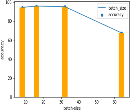
(1) Effect of Batch Size
Batch size defines the number of input samples that are passed on to the network. Batch size is also an influencing parameter which determines the accuracy of classification. Larger the batch size, more time it takes for the training of dataset, and eventually the accuracy of the model decreases and also affects the memory requirement. So, we should be very careful when choosing the batch size. This model is executed with the following batch sizes: 8,16,32,64. The model’s accuracy is increased when there is an increase in the batch size from 8 to 16, slightly decreased at 32, and decreased at a batch size of 64. It is observed that at batch size 16, the model produced the highest accuracy which is shown in Figure 4.
Figure 4. Effects of Batch size
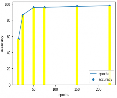
(2) Effect of Number of epochs
Epochs are nothing but the number of iterations. Now by keeping the batch size constant at 16, learning rate at 0.0001 and using Adam optimizer the model is trained at epochs:15, 25, 50, 75, 150, and 225. The Figure 5 shows that 225 epochs gave an accuracy of 97.82%.
Figure 5. Effects of epochs
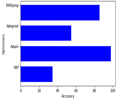
(3) Effect of optimizers
Optimizers are used in optimizing the performance of our model by updating weight parameters which minimize our loss function. Our objective is to reduce the loss of our neural network by enhancing the parameters of our network. The loss function calculates loss by matching the true value and predicted value by a neural network. Here in our work, we evaluated four optimizers, and accuracies are compared in Figure 6 and the best optimizer is determined. The four optimizers used are SGD, Adam, Adagrad, and RMSprop. The Adam optimizer is the best optimizer for our model giving the accuracy of 97.82%. However, RMSprop is also given the accuracy of 85.64%. sgd gave an accuracy of 34.50% and Adagrad of 54.75%.
Figure 6. Effects of optimizers
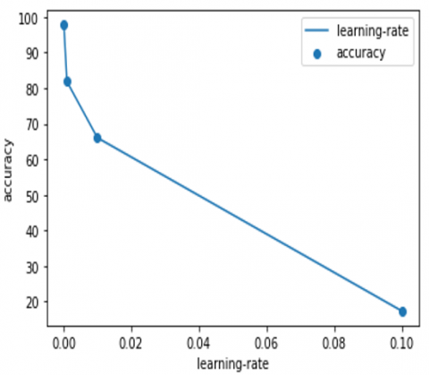
(4) Effect of learning rates
During the training of the neural network, some amount of weights is updated. These weights are called learning rates. This is an important hyperparameter used in the CNN model whose range is between 0.0 and 1.0. In our model, we adopted four learning rates and observed the effects of those learning rates on accuracy. The four learning rates are 0.1, 0.01, 0.001, and 0.0001. From Figure 7, it is observed that upon decreasing the learning rates from 0.1 to 0.0001 the accuracy is improved from 17.36% to 97.82%.
Figure 7. Effects of learning rate
4.1.2 Comparison of classification accuracies of the proposed and transfer learning models
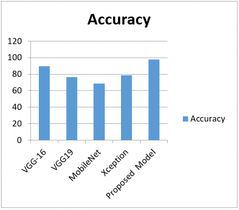
The following are the best combination of hyperparameters that were obtained by hyper-tuning of parameters during the training process: batch size-16, epochs-225, optimizer-Adam, and learning-rate:0.0001. Later, testing was done on the testing dataset that produced an accuracy of 97.82. Figure 8 demonstrates the accuracies obtained for the proposed and transfer learning models comparatively. Among all transfer learning models, it is observed that vgg16 produces high accuracy (89.42%). The accuracy observed in the case of VGG19 and Xception is similar as observed in Figure 8. The proposed model uses a fewer number of filters and parameters that reduce computation time, usage of memory, which makes the proposed model feasible to use in the classification of fresh and rotten fruits.
It is clear from Figure 8 that our CNN model gives the highest accuracy (97.82%). This is due to the combination of convolution and pooling layers, hyperparameters used in the CNN model proposed. A batch normalization layer and an activation function RELU (Rectified Linear Unit) are used in between a conv2d and max-pooling layers which maximize the training and reduces overfitting. Regulalizers are also used to add penalities on the layer while optimizing. A dropout of 0.5 is used. The error loss can be reduced by Adam optimizer. The accuracies obtained in pre-trained models and the proposed CNN model are shown in Table 1. The confusion matrix of the proposed model is shown in Table 2. Comparison study of proposed method with pre-trained models performance is shown in Figure 7. We have compared the accuracy of our model with state of art methods and results proved that the proposed method is accurate than the state of art methods (Table 3) and also transfer learning models (Table 1).
Table 1. Accuracy of pre-trained and proposed model
|
Model |
Accuracy |
|
VGG-16 |
89.42 |
|
VGG19 |
76.18 |
|
MobileNet |
68.72 |
|
Xception |
78.68 |
|
Proposed Model |
97.82 |
Table 2. Confusion matrix of proposed model
|
|
Fresh Apples |
Fresh Bananas |
Fresh Oranges |
Rotten Apples |
Rotten Bananas |
Rotten Oranges |
|
Fresh Apples |
95.80 |
0 |
1.05 |
2.45 |
0 |
0.7 |
|
Fresh Bananas |
0 |
99.35 |
0 |
0 |
0 |
0.65 |
|
Fresh Oranges |
0.9 |
0 |
98.41 |
0.64 |
0 |
0 |
|
Rotten Apples |
2.36 |
0 |
1.7 |
95.94 |
0 |
0 |
|
Rotten Bananas |
0 |
0 |
0.98 |
0 |
98.72 |
0.3 |
|
Rotten Oranges |
0 |
0 |
0.35 |
0 |
1.07 |
98.58 |
Figure 8. Pre-trained models vs proposed model accuracy
Table 3. Comparison of proposed CNN model with state of art methods
|
Author |
Accuracy |
|
Wang, L., Li, A., & Tian, X |
96.7% |
|
Wu, A., Zhu, J., & Ren, T. |
90% |
|
Azizah, L. M., Umayah, S. F., Riyadi, S., Damarjati, C., & Utama, N. A. |
97.5% |
|
Proposed Model |
97.82% |
The classification of fresh and rotten fruits is very important in agricultural fields. In our work, we introduced a model based on CNN and concentrated on building transfer learning models for the task of classification of fresh and rotten fruits. Transfer learning models VGG16, VGG19, MobileNet, and Xception are used in this problem and the accuracies are compared against the proposed CNN model. The effects of different hyper-parameters i.e. batch-size, number of epochs, optimizer, and learning rate are interrogated in this work. The results proved that the CNN model proposed can classify fresh and rotten fruits firmly and produced better accuracy than transfer learning models. Thus, the proposed CNN model can automate the process of human brain in classifying the fresh and rotten fruits with the help of the proposed convolutional neural network model and thus reduces the human errors while classifying fresh and rotten fruits. The accuracy of 97.82% is attained for the proposed CNN model.
The future extent for this work includes increasing varieties of fruits will be taken for classification, so that every fruit farmer will use the system. The work proposed is more useful for fruit yielding farmers for the classification of fresh and rotten fruits in yield so that they can get better cost price at markets.
[1] Reddy C.V.R., Reddy U.S., Kishore K.V.K. (2019). Facial emotion recognition using NLPCA and SVM, Traitement du Signal, 36(1): 13-22. https://doi.org/10.18280/ts.360102
[2] VenkataRamiReddy, C., Kishore, K.K., Bhattacharyya, D., Kim, T.H. (2014). Multi-feature fusion based facial expression classification using DLBP and DCT. International Journal of Software Engineering and Its Applications, 8(9): 55-68. https://doi.org/10.14257/ijseia.2014.8.9.05
[3] Thenmozhi, K., Reddy, U.S. (2019). Crop pest classification based on deep convolutional neural network and transfer learning. Computers and Electronics in Agriculture, 164: 104906. https://doi.org/10.1016/j.compag.2019.104906
[4] Ramireddy, C.V., Kishore, K.K. (2013). Facial expression classification using Kernel based PCA with fused DCT and GWT features. In 2013 IEEE International Conference on Computational Intelligence and Computing Research, pp. 1-6. https://doi.org/10.1016/10.1109/ICCIC.2013.6724211
[5] Reddy, C.V.R., Kishore, K.K., Reddy, U.S., Suneetha, M. (2016). Person identification system using feature level fusion of multi-biometrics. In 2016 IEEE International Conference on Computational Intelligence and Computing Research, pp. 1-6. https://doi.org/10.1109/ICCIC.2016.7919672
[6] Chirra, V.R.R., ReddyUyyala, S., Kolli, V.K.K. (2019). Deep CNN: A machine learning approach for driver drowsiness detection based on eye state. Revue d'Intelligence Artificielle, 33(6): 461-466. https://doi.org/10.18280/ria.330609
[7] Wang, L., Li, A., Tian, X. (2013). Detection of fruit skin defects using machine vision system. In 2013 Sixth International Conference on Business Intelligence and Financial Engineering, pp. 44-48. https://doi.org/10.1109/bife.2013.11
[8] Azizah, L.M.R., Umayah, S.F., Riyadi, S., Damarjati, C., Utama, N.A. (2017). Deep learning implementation using convolutional neural network in mangosteen surface defect detection. In 2017 7th IEEE International Conference on Control System, Computing and Engineering (ICCSCE), pp. 242-246. https://doi.org/10.1109/iccsce.2017.8284412
[9] Wu, A., Zhu, J., Ren, T. (2020). Detection of apple defect using laser-induced light backscattering imaging and convolutional neural network. Computers & Electrical Engineering, 81: 106454. https://doi.org/10.1016/j.compeleceng.2019.106454
[10] Kamilaris, A., Prenafeta-Boldú, F.X. (2018). Deep learning in agriculture: A survey. Computers and Electronics in Agriculture, 147: 70-90. https://doi.org/10.1016/j.compag.2018.02.016
[11] Howard, A.G., Zhu, M., Chen, B., Kalenichenko, D., Wang, W., Weyand, T., Andreetto, M., Adam, H. (2017). Mobilenets: Efficient convolutional neural networks for mobile vision applications. arXiv preprint arXiv: 1704.04861.
[12] Chollet, F. (2017). Xception: Deep learning with depthwise separable convolutions. In Proceedings of the IEEE conference on computer vision and pattern recognition, pp. 1251-1258. https://doi.org/10.1109/cvpr.2017.195