Yakoub Boukhari
© 2020 IIETA. This article is published by IIETA and is licensed under the CC BY 4.0 license (http://creativecommons.org/licenses/by/4.0/).
OPEN ACCESS
The purpose of this work is to predict the mass loss of cement raw materials during the decarbonation process. The mass loss is influenced by the interaction of several parameters such as chemical composition of raw material, particle size, temperature range of decarbonation and time exposed. Therefore, predicting mass loss based on experimental parameters data is often challenging. For this reason, various machine learning algorithms such as deep networks using autoencoder DN-AE, artificial neural networks optimized by particle swarm optimization PSO-ANN, ANN optimized by ant colony optimization ACO-ANN and ANN are proposed to predict the mass loss. In this research, all models have been applied successfully to predict the mass loss with high accuracy. The results obtained have shown the superiority of DN-AE compared to PSO-ANN, ACO-ANN and ANN. In addition, PSO-ANN and ACO-ANN have a better performance than the individual use of ANN. The values of adjusted R2 indicate that 99.11%, 98.66%, 98.27% and 97.03% of data are explained by DN-AE, ACO-ANN, PSO-ANN and ANN respectively with scatter index (SI) less than 0.1 and maximum error less than 3.32%. Finally, the results justify that all models proposed can be employed to predict the mass loss as alternative tools.
ant colony optimization, artificial neural network, autoencoder, decarbonation process, deep neural networks, mass loss, particle swarm optimization
After water, cement is the second-most consumed material on earth. The global cement production around the world is increasing about 3.3 billion tonnes in 2009 [1] and approximately 3.6 billion tonnes in 2012 [2]. The principal raw materials for the manufacture of cement are mainly limestone, clay (alumino-silicate silicates), sand (silica oxide) and iron ore (iron oxide) in definite mass percentages [3]. The limestone which composed mainly of calcium carbonate CaCO3 is thermally decomposed into lime CaO and carbon dioxide CO2 [4] in rotary kilns.
The raw material mixture is heated in a rotary cement kiln and then cooled by fresh air. A small quantity of gypsum is added to obtain the final cements. The process of thermally decomposing raw materials is called decarbonation. In fact, the decarbonation process is a complex phenomenon. In reality, the chemical composition of raw materials, particle size distributions, temperature range throughout the duration of the decarbonation process are most important factors affecting mass loss due to decarbonation. The relation between the mass loss its influence factors is highly complex [5]. Unfortunately, when the problem is complex, it is difficult or even impossible to obtain exact relationship between target and its influence factors.
In recent years, machine learning algorithms are becoming increasingly more important in modelling of complex phenomena where many factors determine the outcome of the process. It is so difficult, even impossible, to predict target outputs with simple statistical models [6]. One of the major advantages of machine learning algorithm is that it does not need the explicit knowledge of chemical and physical behavior of phenomena [7]. It can be used without knowing the exact mathematical expressions between inputs and output, it only needs to be trained by sufficient training data and optimal parameters to predict the target.
In the present study, various models such as Deep Networks using Auto-Encoder (DN-AE), Artificial Neural Network (ANN), Artificial Neural Network combined with Particle Swarm Optimization algorithm (PSO-ANN) and Ant Colony Optimization (ACO) combined with Artificial Neural Network (ACO-ANN) are used to predict the mass loss of cement raw materials due to decarbonation process. These algorithms are intelligent methodologies that have shown successful and promising results in the domains of modelling and prediction [8] and can be useful and powerful alternative [9]. DN-AE has achieved a good prediction performance on limited protein phosphorylation [10]. PSO-ANN shows good results in the prediction of gas measurement [11] and in the modelling global solar radiation [12]. The ACO combined with ANN has strong predictive ability. It is successfully used to predict of NOx and soot emissions from a diesel engine [13]. ANN is widely used to model highly non-linear and complicated phenomena [14]. It can predict the pitting corrosion in presence of inhibitors with surprising accuracy [15].
The rest of this paper is constructed as follows. Section 2 aims to give a brief overview about models theory. Section 3 describes the materials and experimental methods used. The results obtained are discussed and compared with experimental results in section 4. Finally, section 5 presents our conclusions.
2.1 Artificial Neural Networks (ANN)
The artificial neural networks ANN are inspired from the morphology of biological nervous systems to emulate the functioning of the brain with high capability to learn and to predict based on learning stage. The artificial neural networks consist of multilayer: input layer, output layer and the layer between the input layer and the output layer is named the hidden layer [16]. Generally, there is currently no theoretical criteria adequate for choosing an appropriate number of hidden layer. In In many cases, the neural networks with a unique hidden layer are capable to any continuous function to any desired performance [17]. Each layer is formed by one or more simple processing units called neurons. These neurons are connected to every node in the next layer by some weighted links and bias. In addition, neurons belonging to the same layer are not connected with each other. There are no rules to calculating a suitable number of neurons in the hidden layer. More specifically, the default number of neurons in hidden layer is set to 10. The response (output) of a neuron in hidden layer and output is calculated by activation function which often called transfer function.
The artificial neural network trained using a back propagation (BP) algorithm is most popular and widely used [18]. The evaluation of the artificial neural network is divided into two stages: the first one is feed forward stage and second one is back propagation stage. The back propagation (BP) algorithm is used for weight adjustment [19] to reduce error between experimental values and predicted values. The weight and the thresholds of the artificial neural network are randomly initialized as a value from 0 to 1.
In general, the aim of the training is to choose the optimum parameters such as optimal the number of the hidden layer, optimum nodes number of hidden layers, transfer functions of both hidden and output layers.
2.2 Particle Swarm Optimization - Artificial Neural Networks (PSO-ANN)
The Artificial Neural Networks (ANN) are able efficiently to solve complex problems effectively and efficiently. However, it has some problems during the training phase such trapping at local minima instead of getting the global minimum and convergence speed is slow. In order to overcome this deficiency, the particle swarm optimisation (PSO) algorithm are used to find of the network parameters as weights and thresholds, and to avoid trapping in local minima.
Particle Swarm Optimization - Artificial Neural Networks (PSO-ANN) is a hybrid combination of artificial neural network and particle swarm optimization. PSO algorithm is one of global search methods based stochastic optimisation method. It is proved that PSO algorithm is able to obtain good results in a faster and cheaper way compared with other stochastic technique. The basic idea of PSO algorithm is to imitate the behavior of fish schooling or bird flocking searching food and to guide of particles towards the best promising areas of the search space. PSO algorithm is employed to optimize and to train ANN [20]. It consists of number individuals, called particles. Each particle is considered as a solution. It is characterised by the position and velocity which will be changed and update to find the particle best value and global best value. The solution is initially random generated. The new solutions are updated and are evaluated at each iteration [21]. The operation is repeated until the best solution is reached or given stopping criterion is fulfilled. The greatest advantages of PSO algorithm are that it is very easy to program and has a small number of adjustable parameters. The most popular adjustable parameters of PSO algorithm are population size and iteration number.
2.3 Ant Colony Optimization - Artificial Neural Network (ACO-ANN)
Ant Colony Optimization (ACO) is combined with Artificial Neural Network like PSO algorithms to develop and to optimize ANN architectures. The risk of getting stuck in local optima is sharply reduced by ACO algorithm [22].
Ant Colony Optimization (ACO) is considered as a powerful optimization tool [23] which is used to solve different optimisations problems. It is inspired by the behavior of ants. In nature, ants are able to search for an optimal and shortest trajectory (edge) between their nest and food source. Each ant moves randomly through all to find the food source. When ant find a food leave behind a chemical substance on the ground, called pheromone. The quantity, the quality and the distance of the food source are related to the quantity of the laid pheromone. The pheromone evaporation of pheromone [24] over the time plays an important role to fall into the local optimum and to avoid the rapid convergence to a local optimal. Without evaporation of pheromone, the first paths selected by the first ant is extremely attractive to the other ants, and consequently, the research space could be limited. The path which contained more quantity of pheromone is becoming the main path. In each iteration with sufficient number of ants, the quantity of pheromone is updated and reinforced which help to attain more precise solutions.
The main advantage of ACO algorithm is to converge rapidly to optimal solutions without falling into a local optimum. The optimal performance of the ACO mainly depends on suitable parameters settings. The main parameters of ACO are number of ants per iteration, number iterations and evaporation rate of pheromone.
2.4 Deep Networks using Autoencoder (DN-AE)
The distinction between deep learning networks and artificial neural networks lies in their depth and more complex of connecting ways between layers with more number of neurons. Deep Network using Auto-Encoder [25] is one of most popular deep neural networks which can learn the underlying structure of the dataset. It comprises an input layer, one or more hidden layer and an output layer. The training phase is composed by two procedures. The first one is pre-training by one or several autoencoders layers AEs and the second is the training by softmax layer. These multiple layers are stacked together to form DN-AE by stack function.
Autoencoder (AE) layer is a specific type of artificial neural network composed of an encoder and a decoder. It is used to extract complex feature from data complex and to generate new data [26] with as much accuracy and low error as possible. The output of the first layer AE is taken as the input of the following layer. The main settings pre-training parameters of autoencoder layers are: the number of AE layers, size of hidden layer, iteration number, encoder transfer function, decoder transfer function. Then the output of the last AEs is taken as input of the softmax layer. The undesired performance of DN-AE may appear when the number of AE layers is not well selected. In some situation, using more than one AE layers can enhance the accuracy of results [27] especially when the number of inputs increases.
Softmax layer is the last layer [28] used in deep neural networks. It is used to train the deep network [29] and improve the accuracy during the learning by minimizing the loss function. The most important parameters of softmax layer are maximum number of training iterations and type of loss functions. The cross entropy loss is usually used as loss function [30] instead of mean square error (MSE).
3.1 Materials and experiments
Cements are chemically composed by the main following oxides: calcium oxide CaO, silica SiO2 and alumina Al2O3, magnesium oxide MgO, and iron oxide Fe2O3 from limestone, clay, sand and iron ore. The raw materials used in this study are subjected to chemical treatments. Chemical composition of each raw material used is shown in Table 1. Four samples are carefully prepared with different combination of raw materials. The raw materials mix composition (% by weight) of each sample are summarised in Table 2. Each sample is separated by using a series of sieves with different mesh into the different particles sizes: 350µm, 250µm, 125µm and 71µm.
Table 1. Chemical composition (% by weight) for each raw material used
|
Raw material |
SiO2 |
CaO |
MgO |
Fe2O3 |
Al2O3 |
|
Limestone |
3.96 |
92.62 |
0.99 |
0.65 |
1.78 |
|
Clay |
58.61 |
12.53 |
3.49 |
7.43 |
17.94 |
|
Sand |
93.37 |
3.59 |
0.34 |
1.10 |
1.60 |
|
Iron ore |
24.12 |
14.94 |
2.03 |
53.34 |
5.57 |
Table 2. Raw materials mixture composition (% by weight) of each sample
|
Sample |
limestone |
Sand |
Clay |
Iron ore |
|
1 |
100 |
- |
- |
- |
|
2 |
85 |
15 |
- |
- |
|
3 |
83 |
15 |
2 |
- |
|
4 |
82.5 |
14.5 |
2 |
1 |
Table 3. Every sample with different combination of grain size and exposed time is heated at 1000℃
|
Particle size (µm) |
Time (min) |
||||
|
5 |
10 |
15 |
20 |
30 |
|
|
71 |
+ |
+ |
+ |
+ |
+ |
|
125 |
+ |
+ |
+ |
+ |
+ |
|
250 |
+ |
+ |
+ |
+ |
+ |
|
310 |
+ |
+ |
+ |
+ |
+ |
Table 4. First and the last samples with particles size of 350 µm are heated at various temperatures during 20-min
|
Sample |
Temperature (℃) |
||||
|
600 |
700 |
800 |
900 |
1000 |
|
|
Sample 1 |
+ |
+ |
+ |
+ |
+ |
|
Sample 4 |
+ |
+ |
+ |
+ |
+ |
In practice, this study consists of two parts: first part, each sample with different grain size distribution is heated at high 1000℃ during various time from 5 to 30 min in a laboratory muffle furnace as shown in Table 3. Second part, only the first sample and the last sample with grain size of 350 µm are subjected to a wide temperature range of 600–1000℃ with a step size of 100℃ during period 20-min as shown in Table 4.
Measurements of the mass loss were carried out under the influence of various experimental conditions, including particles size distribution, exposed time, chemical composition and temperature. Each sample are carefully weighed before and after decarbonation process to quantify the mass loss. The mass loss was calculated as follows:
$m l(\%)=\frac{m_{i}-m_{f}}{m_{i}} \times 100$ (1)
where, mi and mf represent respectively the weight of a sample before and after decarbonation process as described in previous work [7].
3.2 Data acquisition
Dataset obtained in the first case is organized in a table (20 rows x 3 columns) for each sample. Each row presents experience. Two first columns namely particle size distributions, exposed time are chosen as the inputs of each model. The last column called mass loss is used as target. Dataset obtained in the second case is collected in the table (10 rows x 3 columns).
All dataset obtained in both cases are joined to form total dataset (90 rows x 10 columns). The columns from 1 to 9 are as follows: the particle size distributions of each samples, exposed time of each sample and temperature. The nine columns are the inputs. The column 10 called mass loss is taken as output.
Each dataset obtained are separated into two parts: training dataset and testing dataset. Training dataset is exploited to construct the model and testing dataset (remaining data) is used to test its generalization capability. There are several percentages of training dataset and testing dataset are reported in the literature [31, 32]. In this study, the dataset is randomly separated into two subsets. The dataset for the training is chosen randomly from 2/3 of the dataset and the remaining of dataset (1/3) are used to evaluate the generalization capability of model.
In this paper, all data is necessary normalized before training the models within a uniform interval of [0–1]. The normalization formula is given as follows:
${{x}_{norm}}=\frac{x-{{x}_{\min }}}{{{x}_{\max }}-{{x}_{\min }}}$ (2)
where, xnorm is variable normalised, xmax is maximum value and xmin is minimum value.
3.3 Predictive performances
Some performance criteria are statistically measured to evaluate the prediction capacity such as R2 (coefficient of determination), RMSE (root mean squared error) [33], MAPE (mean absolute percent error) and adjusted R2 to evaluate the prediction capacity [34] which are defined as follows:
$RMSE=\sqrt{\sum\limits_{i=1}^{N}{\frac{{{({{Y}_{i(\exp )}}-{{Y}_{i(pred)}})}^{2}}}{N}}}$ (3)
${{R}^{2}}=1-\left( {\left( \sum\limits_{i=1}^{N}{{{({{Y}_{i(\exp )}}-{{Y}_{i(pred)}})}^{2}}} \right)}/{\left( \sum\limits_{i=1}^{N}{{{({{Y}_{i(\exp )}}-{{Y}_{i(mean)}})}^{2}}} \right)}\; \right)$ (4)
$MAPE=\frac{100}{N}\sum\limits_{i=1}^{N}{\left| \frac{{{Y}_{i(\exp )}}-{{Y}_{i(pred)}}}{{{Y}_{i(\exp )}}} \right|}$ (5)
where, N is the number of data, Yi(exp) and Yi(pred) indicate the experimental and predicted values respectively, Yi(mean) is the mean value of experimental data points.
While the adjusted R2 is given by the following equation:
$R_{adj}^{2}=1-(1-{{R}^{2}})\times \left( \frac{N-1}{N-P-1} \right)$ (6)
where, N is number of data, P is number of variables and R2 is the coefficient of determination given in Eq. (4).
The predictions are excellent if the values of adjusted R2 and R2 are found very close to 1. The models are capable of predicting with a high accuracy when values of RMSE and MAPE are found very close to zero.
In terms of scatter index (SI) [35, 36] which is given in Eq. (7). The performance of model is excellent when SI is inferior to 0.1; good if SI between 0.1and 0.2, and poor if SI is superior to 0.3. All performance indicators are calculated between experimental values and predictions values.
$SI=\frac{RMSE}{{{Y}_{i(mean)}}}$ (7)
where, RMSE is given in Eq. (3) and Yi(mean) is the mean value of experimental data points.
In general, machine learning algorithms proposed in this study with adjustable parameters are usually able to approximate any nonlinear problems. The optimal parameters for each model are determined experimentally after several tests. The accuracy of each machine learning algorithm is evaluated during a phase testing, because it is much easy to realize a high accuracy during a phase training without improving generalisation capability. All machine learning algorithms are implemented in Matlab 2018a.
The results and discussion are divided into parts: predicting totally and predicting separately. The first part discusses the predicted results of overall data in more detail. The second parts are discussed separately the predicted results obtained in previously parts as summarised in Tables 3 in less detail than first part in order to check and to confirm the accuracy of each model.
4.1 Predicting totally
As described above, total dataset at the end of experimental part are collected in table (90 rows x 10 columns). The number of inputs and output are 9 and 1 respectively. It is evident that the training of models is becoming more complex when the number of inputs increased.
4.1.1 ANN result
Generally, it is better to choose more than one hidden layer in this situation. The optimal architecture network of ANN is 2 hidden layers with 12 neurons in each one (9:12:12:1), with ‘tansig’ (hyperbolic tangent sigmoid) as activation function and ‘purelin’ (linear) as activation function for output layer.
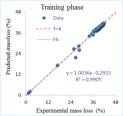
The experimentally mass loss and those predicted by applying ANN for both training and testing phases are presented in Figure 1 and Figure 2. These figures illustrate good agreement between experimental mass loss and predicted values for training and testing phases. It is also observed that the points are close to the straight diagonal line. The R2 values are 0.9905 for the training and 0.9714 for the testing phase. These figures with high values of R2 indicate excellent correlation between the experimental and predicted values of mass loss and approve the good predictive capability of ANN model.
Table 5 illustrate the remaining criteria used. The values of R2 adjusted mean that ANN is able to effectively predict up to 99% and 97.03% of training and testing data respectively with SI less than 0.1 and low value of MAPE and RMSE. These criteria indicate excellent performance of ANN. The results obtained is expected due to high learning capability and great flexibility of ANN model.
Figure 1. Experimental and predicted mass loss at training phase of ANN
Figure 2. Experimental and predicted mass loss at testing phase of ANN
Table 5. Performance criteria obtained by ANN
|
|
R² adj |
MAPE |
RMSE |
SI |
|
Train |
99.04% |
1.48% |
0.7825 |
0.0213 |
|
Test |
97.03% |
3.31% |
1.5327 |
0.0413 |
4.1.2 PSO-ANN result
The optimal neural network structure of PSO-ANN is the same as for the ANN non-optimised used in the previously part (9:12:12:1) in order to compare the prediction accuracy. The main optimum parameters of the PSO-ANN algorithm are: population size is 18 and iteration number is 12.
Figure 3 and Figure 4 show the results obtained of the PSO-ANN models for the prediction of mass loss of testing and training. It is clearly observed that the fit line is shown practically superimposed on the plot of full equality. The R2 values are equal to 0.9974 and 0.9833 for testing phase which reflect a good fit. The values of PSO-ANN model show high potential in learning training phase and good generalization capability.
The other performance criteria are illustrated in Table 6. The adjusted R2 values indicating that the PSO-ANN explained 99.73% of training dataset and 98.26% of testing dataset. Therefore, the SI value less than 0.1 indicates excellent accuracy during both phases. The best result obtained by PSO-ANN is due to the better optimization by PSO and high learning capability of the ANN.
Figure 3. Experimental and predicted mass loss at training phase of PSO-ANN
Figure 4. Experimental and predicted mass loss at testing phase of PSO-ANN
Table 6. Performance criteria obtained by PSO-ANN
|
|
R² adj |
MAPE |
RMSE |
SI |
|
Train |
99.73% |
1.48% |
0.4236 |
0.01146 |
|
Test |
98.26% |
3.00% |
1.1822 |
0.03222 |
4.1.3 ACO-ANN result
Generally, the optimal architecture network of ACO-ANN is similarly to those used to design the PSO-ANN and ANN (9:12:12:1). The main appropriate parameters of ACO-ANN are: number of ants per iteration is 12, number iterations are 14 and evaporation rate of pheromone is 0.8.
The results obtained by applying ACO-ANN for both training and testing phases are presented in Figure 5 and Figure 6. It is clear that almost of points lie exactly on a straight line. The high values of R2 obtained during the both phases are 0.9961 for training and 0.9870 for testing phases. These values which are close to 1, indicate a strong and robust correlation between experimental and predicted mass loss. In addition, the regression line is generally equal to the line Y=X. It is clear that ACO-ANN can predict mass loss with high prediction precision.
Figure 5. Experimental and predicted mass loss at training phase of ACO-ANN
Figure 6. Experimental and predicted mass loss at testing phase of ACO-ANN
The remaining of performance criteria are listed in Table 7. The adjusted R2 values show that there are only 0.39% of training and 1.34% of testing are not explained ACO-ANN with SI value less than 0.1 and error less than 2.53%. The best the predictive accuracy of ACO-ANN is related to the strong searching of ACO which improve and increase the learning ability of the ANN.
Table 7. Performance criteria obtained by ACO-ANN
|
|
R² adj |
MAPE |
RMSE |
SI |
|
Train |
99.61% |
1.33% |
0.5073 |
0.0138 |
|
Test |
98.65 % |
2.53% |
1.0555 |
0.0286 |
4.1.4 DN-AE result
Similarly, the optimal parameters of the DN-AE for achieving a more precise accuracy is: number of AEs layers is 2 with 20 neurons in each one and 850 iterations, encoder and decoder transfer function are ‘logsig’ (log-sigmoid) and ‘purelin’ respectively, softmax layer with cross entropy as loss function and 750 iterations.
The experimental versus DN-AE model predicted values of mass loss are represented in Figure 7 and Figure 8 respectively. It is clearly seen from these figures that predicted values using DN-AE are in suitable agreement with experimental of mass loss results for both phases. Moreover, the data dispersion generally lies around the identity line, indicating the excellent closeness between predicted and experimental values. The goodness of fit is given by the values of R2, which are 0.9912 and 0.9914 for training and testing respectively. These R2 values indicate an excellent correlation and confirm the excellent predictive ability of DN-AE.
Figure 7. Experimental and predicted mass loss at training phase of DN-AE
Figure 8. Experimental and predicted mass loss at testing phase of DN-AE
The other performance criteria for two phases are presented in Table 8. According to the values of adjusted R2, there are 99.11% of training and testing data can explain by DN-AE model. It is also clear that the values of R2 and adjusted R2 are close to 1 while the RMSE, SI and MAPE, are close 0. These values mean a very accurate prediction model. The robust learning and generalisation ability of the DN-AE is emphasised. This high performance mainly comes from the deep learning architectures, features extraction capability and highly representative data by autoencoders layers.
Table 8. Performance criteria obtained by DN-AE
|
|
R² adj |
MAPE |
RMSE |
SI |
|
Train |
99,11% |
2,27% |
0,7918 |
0,0219 |
|
Test |
99.11% |
2,18% |
0,6948 |
0,0181 |
4.2 Predicting separately
Each algorithm is applied to each sample to predict the effect of chemical composition as mentioned in Table 3. In the same way, the ACO-ANN, PSO-ANN and ANN have same optimal architecture network (2:6:1) with tansig and purelin transfer function in a hidden layer and output layer respectively. The other main parameters of ACO-ANN are 6 ants, 4 iterations and 0.8 evaporation rate. The other main parameters of PSO-ANN are 8 particles (population size) and 5 iterations.
The optimal parameters of the DN-AE are as flowing: 6 neurons in AE layer, 150 iterations, encoder and decoder transfer function are logsig and purelin respectively, softmax layer with cross entropy as loss function and 350 iterations.
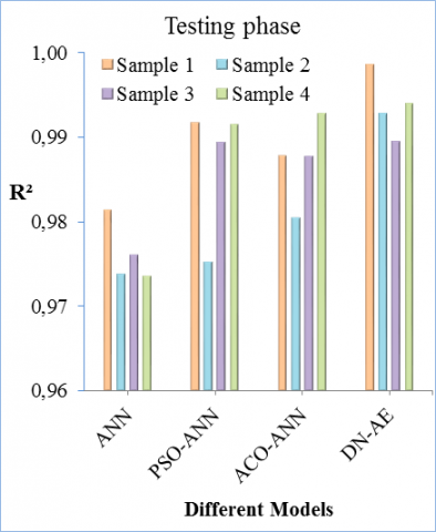
The values of MAPE and R2 of testing dataset of various models obtained from all samples are shown in Figure 9 and Figure 10.
It is observed from these figures that there is an adequate agreement obtained by all models between the predicted values of mass loss and experimental values. The value of R2 indicate that the mass loss predicted by DN-AE is much closer to then experimentally result than those predicted by other models. The values of MAPE and R2 of ANN are slightly improved when the ANN combined with PSO or ACO algorithms. It is clear that the best accuracy is obtained by DN-AE. The MAPE values are varied between 0.25% as the smallest and 3.52% largest value. Furthermore, the R2 values are varied between 0.9985 as maximum value and 0.9737 as the minimum value. It is clear that the lowest R2 is obtained by ANN and the highest by DN-AE.
The MAPE and R2 values of PSO-ANN and ACO-ANN are slightly better than the pure ANN. The superiority predictive accuracy of hybrid PSO-ANN and ACO-ANN compared to ANN can be attributed to its powerful search capabilities by PSO and ACO algorithms. ACO-ANN and PSO-ANN have practically same performance. The best performance obtained by DN-AE is due to applying the deep learning by AE layer. It is concluded that all models are very promising models for mass loss prediction in terms of predictive accuracy for each sample.
The remaining performance criteria on the training and testing datasets for the various models are reported in Table 9. It can be seen that the performance accuracy obtained by four models are quite different. The R2 adjusted values obtained in the testing datasets for DN-AE, ACO-ANN, PSO-ANN and ANN are more than 96.84%, 97.04%, 97.65% and 98.73% with SI less 0.1. Consequently, the values of performance criteria indicate the effectiveness and high accuracy of all models even with small data size due to their robustness and flexibility.
Figure 9. Comparison between all models in term of R2 for all samples
Figure 10. Comparison between all models in term of MAPE for all samples
Table 9. Performance criteria (Perf-Crit) for testing phases of all models for each sample (S)
|
S |
Perf-Crit |
Testing phase |
|||
|
ANN |
ACO-ANN |
PSO-ANN |
DN-AE |
||
|
1 |
R2 adj |
97.77% |
99.01% |
98.54% |
99.82% |
|
RMSE |
0,9187 |
1.1978 |
0.1931 |
0.2230 |
|
|
SI |
0.0252 |
0.0323 |
0.0051 |
0.0061 |
|
|
2 |
R2 adj |
96.86% |
97.04% |
97.65% |
99.13% |
|
RMSE |
1.9449 |
0.6284 |
0.9979 |
0.0081 |
|
|
SI |
0.0525 |
0.0168 |
0.0268 |
0.0085 |
|
|
3 |
R2 adj |
97.14% |
98.72% |
98.52% |
98.73% |
|
RMSE |
1.3061 |
0.4501 |
0.5103 |
0.0085 |
|
|
SI |
0.0325 |
0.0113 |
0.0127 |
0.1762 |
|
|
4 |
R2 adj |
96.84% |
98.97% |
99.13% |
99.27% |
|
RMSE |
1.6378 |
0.1629 |
0.2688 |
0.1225 |
|
|
SI |
0.0402 |
0.0040 |
0.0066 |
0.0030 |
|
4.3 Comparison between the different models
A comparative study between DN-AE, ACO-ANN, PSO-ANN and ANN models used to predict of mass loss of different raw materials are conducted of in terms of MAPE and R2 to compare the generalization ability of models. It includes all data mentioned in section 4.1 above. The results of the compared models are shown in Figure 11. It is clear that the increasing of data enlarges the complexity in adjusting parameters between the layers. The determination coefficient R2 for testing dataset by DN-AE, ACO-ANN, PSO-ANN and ANN are 0.9914, 0.9870, 0.9833, and 0.9714 respectively. The results based on R2 show an excellent concordance between the predicted values and experimental values. The maximum error value which is obtained by ANN is 3.32%, whereas the lowest error value from DN-AE is 2.18%.
Figure 11. Comparison between all models in term of MAPE and R2 at testing phase of total dataset
The upper predictive accuracy of DN-AE can be attributed to its deep learning process by two AE layers which are able to approximate any non-linear system. It is clear that there is no significant difference between ACO-ANN and PSO-ANN in terms of R2 and a slight difference in terms of MAPE. It seems that PSO-ANN or ACO-ANN is better than ANN non-optimised. Thus, the PSO or ACO can improve the performance precision of ANN effectively by optimisation its parameters. ANN is proven to have a performance nearly equivalent to other models. Furthermore, it is a very competitive relative to other models due to high learning capability and easy to develop nonlinear function.
The performance criteria of all dataset which are summarised in Table 5, Table 6, Table 7 and Table 8 reveal that more than 97% can be explained by all models. Also, the performance of all models is excellent with SI less than 0.1 and error less 3.32%. Overall, the values of performance criteria indicate that all models are considered to be able to predict the mass loss of cement raw materials caused by decarbonation process with a high generalization capability. All machine learning algorithms can be used as alternative tools to experimental determination and are easily be applied on large or small datasets.
In the present study, DN-AE, ACO-ANN, PSO-ANN and ANN are used to predict the mass loss of cement raw material due to decarbonation process which is influenced by interaction of a number of factors. The results obtained in all cases and under the optimum parameters of each model demonstrate that all models can be successfully applied to predict the mass loss. The prediction capability of DN-AE has shown its superiority over ACO-ANN, PSO-ANN and ANN with comparative high value of R2 and R2 adjusted with less value of MAPE, RMSE and SI. The predictive accuracy of DN-AE can be attributed to its deep learning process and features extraction capability of autoencoders layers. There is only a slight difference between ACO-ANN and PSO-ANN. Moreover, the performance acquired by ANN optimised by PSO or ACO is better compared to ANN non-optimised. It is expected because ACO or PSO is able to find the optimum parameters of ANN and to avoid converging to a local optimum. Furthermore, ANN is proven to have an excellent performance nearly equivalent to DN-AE, ACO-ANN and PSO-ANN.
According to the values of R2 adjusted of DN-AE, ACO-ANN, PSO-ANN and ANN obtained with a total dataset, there are only 0.89%, 1.34%, 1.73% and 2.97% of the total datasets respectively are not explained by this model. The highest error which is obtained by ANN is 3.32%, whereas the lowest error value from DN-AE is 2.18%. The values of SI obtained by all models which are small than 0.1 are indicative of the excellent accuracy. Finally, all machine learning algorithms proposed can be used as alternative tools to experimental determination of mass loss.
[1] Feiz, R., Ammenberg, J., Baas, L., Eklund, M., Helgstand, A., Marshall, R. (2018). Improving the CO2 performance of cement, part 1: Utilizing life-cycle assessment and key performance indicators to assess development within the cement industry. Journal of Cleaner Production, 98: 272-281. https://doi.org/10.1016/j.jclepro.2014.01.083
[2] Rashad, A.M. (2015). Potential use of phosphor gypsum in alkali-activated fly ash under the effects of elevated temperatures and thermal shock cycles. Journal of Cleaner Production, 87: 717-725. https://doi.org/10.1016/j.jclepro.2014.09.080
[3] Young, G., Yang, M. (2019). Preparation and characterization of Portland cement clinker from iron ore tailings. Construction and Building Materials, 197: 152-156. https://doi.org/10.1016/j.conbuildmat.2018.11.236
[4] Shen, L., Gao, T., Zhao, J., Limao, W., Lan, W., Liu, L., Chen, F., Xue, J. (2014). Factory-level measurements on CO2 emission factors of cement production in China. Renewable and Sustainable Energy Reviews, 34: 337-349. https://doi.org/10.1016/j.rser.2014.03.025
[5] Carter, L.B., Dasgupta, R. (2018). Decarbonation in the Ca-Mg-Fe carbonate system at mid-crustal pressure as a function of temperature and assimilation with arc magmas – Implications for long-term climate. Chemical Geology, 492: 30-48. https://doi.org/10.1016/j.chemgeo.2018.05.024
[6] Boukhari, Y., Boucherit, M.N., Zaabat, M., Amzert, S., Brahimi, K. (2017). Artificial intelligence to predict inhibition performance of pitting corrosion. Journal of Fundamental and Applied Sciences, 9(1): 308-322. http://dx.doi.org/10.4314/jfas.v9i1.19
[7] Boukhari, Y. (2020). Using intelligent models to predict weight loss of raw materials during cement clinker production. Revue d'Intelligence Artificielle, 34(1): 101-110. https://doi.org/10.18280/ria.340114
[8] Boukhari, Y., Boucherit, M.N., Zaabat, M., Amzert, S., Brahimi, K. (2018). Optimization of learning algorithms in the prediction of pitting corrosion. Journal of Engineering Science and Technology, 13(5): 1153-1164.
[9] Boucherit, M.N., Amzert, S.A., Arbaoui, F., Boukhari, Y., Brahimi, A., Younsi, A. (2019). Modelling input data interactions for the optimization of artificial neural networks used in the prediction of pitting corrosion. Anti-Corrosion Methods and Materials, 66(4): 369-378. https://doi.org/10.1108/ACMM-07-2018-1976
[10] Lumbanraja, F.R., Mahesworo, B., Cenggoro, T.W., Budiarto, A., Pardameanbd, B. (2019). An evaluation of deep neural network performance on limited protein phosphorylation site prediction data. Procedia Computer Science, 157: 25-30. https://doi.org/10.1016/j.procs.2019.08.137
[11] Rosli, N.S., Ibrahim, R., Ismail, I. (2017). Intelligent prediction system for gas metering system using particle swarm optimization in training neural network. Procedia Computer Science, 105: 165-169. https://doi.org/10.1016/j.procs.2017.01.197
[12] Mohandes, M.A. (2010). Modeling global solar radiation using Particle Swarm Optimization (PSO). Solar Energy, 86(11): 3137-3145. https://doi.org/10.1016/j.solener.2012.08.005
[13] Mohammadhassani, J., Dadvand, A., Khalilaryab, S., Solimanpurb, M. (2015). Prediction and reduction of diesel engine emissions using a combined ANN–ACO method. Applied Soft Computing, 34: 139-150. https://doi.org/10.1016/j.asoc.2015.04.059
[14] Tiryaki, B. (2008). Predicting intact rock strength for mechanical excavation using multivariate statistics, artificial neural networks, and regression trees. Engineering Geology, 99(1-2): 51-60. https://doi.org/10.1016/j.enggeo.2008.02.003
[15] Boucherit, M.N., Amzert, S.A., Arbaoui, F., Hanini, S., Hammache, A. (2008). Pitting corrosion in presence of inhibitors and oxidants. Anti-Corrosion Methods and Materials, 55(3): 115-122. https://doi.org/10.1108/00035590810870419
[16] Khoshroo, A., Emrouznejad, A., Ghaffarizadeh, A., Kasraei, M., Omid, M. (2018). Sensitivity analysis of energy inputs in crop production using artificial neural networks. Journal of Cleaner Production, 197(1): 992-998. https://doi.org/10.1016/j.jclepro.2018.05.249
[17] Hornik, K., Stinchcombe, M., White, H. (1989). Multilayer feedforward networks are universal approximators. Neural Networks, 2(5): 359-366. https://doi.org/10.1016/0893-6080(89)90020-8
[18] Huang, Q., Cui, L. (2019). Design and application of face recognition algorithm based on improved backpropagation neural network. Revue d'Intelligence Artificielle, 33(1): 25-32. https://doi.org/10.18280/ria.330105
[19] Ye, Z., Kim, M.K. (2018). Predicting electricity consumption in a building using an optimized back-propagation and Levenberg–Marquardt back-propagation neural network: Case study of a shopping mall in China. Sustainable Cities and Society, 42: 176-183. https://doi.org/10.1016/j.scs.2018.05.050
[20] Lazzús, J.A. (2013). Neural network-particle swarm modeling to predict thermal properties. Mathematical and Computer Modelling, 57(9-10): 2408-2418. https://doi.org/10.1016/j.mcm.2012.01.003
[21] Fonna, S., Huzni, S., Ridha, M., Ariffin, A.K. (2013). Inverse analysis using particle swarm optimization for detecting corrosion profile of rebar in concrete structure. Engineering Analysis with Boundary Elements, 37(3): 585-593. https://doi.org/10.1016/j.enganabound.2013.01.005
[22] Liu, Y.P., Wu, M.G., Qian, J.X. (2007). Predicting coal ash fusion temperature based on its chemical composition using ACO-BP neural network. Thermochimica Acta, 454(1): 64-68. https://doi.org/10.1016/j.tca.2006.10.026
[23] Jovanovica, R., Tubab, M., Voß, S. (2019). An efficient ant colony optimization algorithm for the blocks relocation problem. European Journal of Operational Research, 274(1): 78-90. https://doi.org/10.1016/j.ejor.2018.09.038
[24] Bamdad, K., Cholette, M.E., Guan, L., Bell, J. (2017). Ant colony algorithm for building energy optimisation problems and comparison with benchmark algorithms. Energy and Buildings, 154: 404-414. https://doi.org/10.1016/j.enbuild.2017.08.071
[25] Ronao, C.A., Cho, S.B. (2016). Human activity recognition with smartphone sensors using deep learning neural networks. Expert Systems with Applications, 59: 235-244. https://doi.org/10.1016/j.eswa.2016.04.032
[26] Görgel, P., Simsek, A. (2019). Face recognition via Deep Stacked Denoising Sparse Autoencoders (DSDSA). Applied Mathematics and Computation, 355: 325-342. https://doi.org/10.1016/j.amc.2019.02.071
[27] Li, G., Han, D., Wang, C., Hu, W., Vince, D.C., Wang, Y.P. (2020). Application of deep canonically correlated sparse autoencoder for the classification of schizophrenia. Computer Methods and Programs in Biomedicine, 183: 105073. https://doi.org/10.1016/j.cmpb.2019.105073
[28] Caliskan, A., Yuksel, M.E., Badem, H., Basturk, A. (2018). Performance improvement of deep neural network classifiers by a simple training strategy. Engineering Applications of Artificial Intelligence, 67: 14-23. https://doi.org/10.1016/j.engappai.2017.09.002
[29] Li, B., Pi, D. (2019). Learning deep neural networks for node classification. Expert Systems with Applications, 137: 324-334. https://doi.org/10.1016/j.eswa.2019.07.006
[30] Hu, K., Zhang, Z., Niu, X., Zhang, Y., Cao, C., Xiao, F., Gao, X. (2018). Retinal vessel segmentation of color fundus images using multiscale convolutional neural network with an improved cross-entropy loss function. Neurocomputing, 309: 179-191. https://doi.org/10.1016/j.neucom.2018.05.011
[31] Chau, A.L., Li, X., Yu, W. (2014). Support vector machine classification for large datasets using decision tree and Fisher linear discriminant. Future Generation Computer Systems, 36: 57-65. https://doi.org/10.1016/j.future.2013.06.021
[32] Zhou, C., Ding, L.Y., He, R. (2013). PSO-based Elman neural network model for predictive control of air chamber pressure in slurry shield tunneling under Yangtze River. Automation in Construction, 36: 208-317. https://doi.org/10.1016/j.autcon.2013.03.001
[33] Gilan, S.S., Jovein, H.B., Ramezanianpour, A.A. (2012). Hybrid support vector regression – Particle swarm optimization for prediction of compressive strength and RCPT of concretes containing metakaolin. Construction and Building Materials, 34: 321-329. https://doi.org/10.1016/j.conbuildmat.2012.02.038
[34] Khajeh, M., Kaykhaii, M., Sharafi, A. (2013). Application of PSO-artificial neural network and response surface methodology for removal of methylene blue using silver nanoparticles from water samples. Journal of Industrial and Engineering Chemistry, 19(5): 1624-1630. https://doi.org/10.1016/j.jiec.2013.01.033
[35] Stone, R.J. (1993). Improved statistical procedure for the evaluation of solar radiation estimation models. Solar Energy, 51(4): 289-291. https://doi.org/10.1016/0038-092X(93)90124-7
[36] Golafshani, E.M., Behnood, A., Arashpour, M. (2020). Predicting the compressive strength of normal and high-performance concretes using ANN and ANFIS hybridized with grey wolf optimizer. Construction and Building Material, 232: 117-266. https://doi.org/10.1016/j.conbuildmat.2019.117266