Sujuan Li
© 2020 IIETA. This article is published by IIETA and is licensed under the CC BY 4.0 license (http://creativecommons.org/licenses/by/4.0/).
OPEN ACCESS
The forecast of traffic flow state (TFS) is the key to the effective control of roads, especially during large competition events. To enhance the accuracy of TFS forecast, this paper puts forward a way to predict the TFS on the peripheral roads of large competition events, which is based on support vector regression (SVR) and parameter optimization. Firstly, the tensor recovery algorithm was adopted to fill up the missing data. Then, the simulated annealing (SA) algorithm was applied to optimize the SVR parameters like the penalty factor, and the insensitive loss. Next, a TFS forecast model for the road section near large venues was established based on the SVR and the optimized parameters. The example analysis shows that the parameter optimization improved the accuracy of the SVR forecast model, making the predicted results closer to the actual data. The proposed model greatly facilitates the management and control of road traffic during large competition events.
large competition events, traffic flow state (TFS), forecast, parameter optimization, support vector machine (SVM), simulated annealing (SA) algorithm
The forecast of traffic flow state (TFS) is the key to the efficient operation of the traffic system and the effective control of roads. However, the TSF forecast faces high uncertainty under the combined effect of various internal and external factors, which reflect the time-variation, complexity and nonlinearity of the traffic system. It is particularly difficult to predict the short-term TFS when traffic control measures are adopted for large competition events. To overcome the difficulty, the variation law of traffic flow should be determined during large competition events, based on the spatiotemporal correlation of traffic flow data. Once the variation law is obtained, it is possible to find the way to project the TFS on roads in typical scenarios, and help the competent department to control the traffic effectively during large competition events.
By our understanding of traffic state, the TFS is generally considered as continuous. In essence, the forecast of the TFS is to predict the variables, indices and parameters of the TFS. The existing TFS forecast methods generally fall into the following four categories.
Some TFS forecast methods are based on parametric models. These methods estimate the parameters of the future TFS with accurate forecast models. The typical models include linear ones like time series method [1-4], Kalman filtering [5-8] and exponential smoothing, as well as nonlinear ones like wavelet analysis [10-12] and chaos theory [13-15].
Some TFS forecast models are based on nonparametric models. These methods require no accurate model expressions. Instead, the variation law of traffic flow data is mined out from a huge amount of historical or survey data, and used to predict the TFS. Such methods include the k-nearest neighbors (kNN) algorithm [16], decision tree [17-19], etc.
Some TFS forecast methods are based on machine learning models, namely, the neural network (NN) [20-25] and the support vector machine [26-27]. These methods mainly train the model with abundant historical data to obtain the mapping between inputs and outputs.
Some TFS forecast methods combine two or more types of the above methods. Through the combination, the merits of the different methods are retained and the defects are solved, leading to a better prediction accuracy. For example, Park [28] developed a hybrid forecast model for the TFS parameters of expressways based on the radial basis function (RBF) neural network (NN) and the fuzzy c-means (FCM) clustering. Zheng et al. [29] predicted the TFS using the Bayesian network and the NN. Boto-Giralda et al. [30] conducted TFS forecast with wavelet analysis and a self-organizing NN. For TFS prediction, Zhang [31] designed a model coupling the SVM and the seasonal autoregressive integrated moving average (ARIMA) model.
Drawing on the fourth type of TFS forecast methods, this paper fully considers the strengths and weaknesses of multiple prediction models for TFS parameters, and then proposes a TFS forecast method based on support vector regression (SVR). To improve the forecast accuracy, the model parameters were optimized by the SA algorithm, which is suitable to solve largescale combinatorial optimization problems.
This paper mainly tackles the TFS on the peripheral roads of large competition events. The TFS data were collected from a section of Xiangyun Avenue, a high-level trunk road, near Nanchang International Sports Center (NISC), a landmark sports building in Nanchang (Figure 1). The sampling area was selected for two reasons: the traffic state around the NISC directly affects the operation of the entire road network in Nanchang; the TFS on Xiangyun Avenue must be monitored in time, making it safe and rapid for traffic to converge and disperse before and after large competition events.
Figure 1. Location of the NISC
Considering data availability, the mean speed data were collected from the section of Xiangyun Avenue in June, 2017 and taken as the samples for TFS forecast. However, some of the TFS data went missing due to the maloperation of the collection devices and transmission failures. To solve the problem, the spatiotemporal features of the TFS data were analyzed, revealing the multi-mode correlation and spatiotemporal distribution pattern of the data. On this basis, a TFS data tensor model was constructed. Then, the missing data were filled up using the tensor recovery algorithm, which performs full-rank decomposition of low-rank multi-linear matrix.
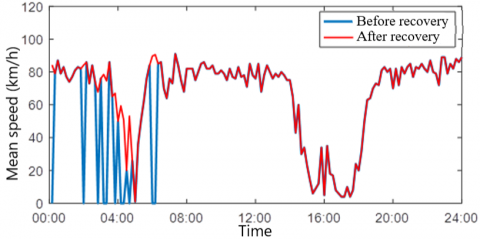
After the TFS data in July were preprocessed, the TFS data were selected from one day (e.g. July 1st) with competition events and another day (e.g. July 13th) without competition events for data recovery. The missing data in the TFS data on the two days were filled up. Figure 2 compares the time series of mean speeds before and after the recovery.
(a) July 13th (without competition events)
(b) July 1st (with competition events)
Figure 2. The time series of mean speeds before and after the recovery
As shown in Figure 2(a), when no competition events took place, the mean speed in the recovered data belong to the same interval as the mean speed of the normal hours, and the recovered data retain the fluctuation in the TFS. As shown in Figure 2(b), when competition events were held, the recovered data also retain the fluctuation in the TFS, and reflect how the road was gradually congested and then become smooth again through the competition events. To sum up, the tensor recovery algorithm has effectively filled up the missing data, and the recovered data reflect the TFS features, whether the competition events took place.
To effectively forecast the real-time TFS, this paper firstly analyzes the TFS data during large competition events, and fills up the missing data by the tensor recovery algorithm. Next, the SA algorithm was employed to optimize the parameters for the SVR forecast model, including the penalty coefficient C, the insensitive loss $\varepsilon$ and the kernel function $\sigma$ . After that, a TFS forecast model was established based on the SVR and the optimal parameters. Finally, the model was applied to predict the TFS in an actual case. The results reveal the effects of parameter optimization on the forecast model, laying a solid basis for traffic control during large competition events. The technical roadmap of this research is given in Figure 3.
Figure 3. Roadmap of TFS forecast based on the SVR and parameter optimization
3.1 SVR model
The SVR model was mainly constructed based on classifiers. Let $T=\left\{\left(x_{i}, y_{j}\right), \cdots\left(x_{l}, y_{l}\right)\right\} \in(X \times Y)^{l}$ be the training set, where $\mathrm{x}_{\mathrm{i}} \in \mathrm{X}=\mathrm{R}^{\mathrm{n}}, \mathrm{y}_{\mathrm{i}} \in \mathrm{Y}=\{-1,1\}$ and $i=1,2, \cdots l$. Let $\left(x_{i+l}^{T}, y_{i+l}-\varepsilon\right)^{T}=\left(x_{i}^{T}, y_{i}-\varepsilon\right)^{T}, i=1,2, \cdots l$. Then, a new training set was obtained as $\left\{\left(\left(x_{1}^{T}, y_{1}^{T}+\varepsilon\right)^{T}, 1\right), \cdots\left(\left(x_{l}^{T}, y_{l}^{T}+\varepsilon\right)^{T}, 1\right)\right.$,$\left(\left(x_{1+1}^{T}, y_{1+1}^{T}+\varepsilon\right)^{T},-1\right), \cdots\left(\left(x_{21}^{T}, y_{21}^{T}+\varepsilon\right)^{T},-1\right)$. In this way, the regression of the original training set is converted into the binary classification of the new training set. Based on the new training set, the optimal classification hyperplane was obtained by the SVM classification. Then, the regression decision function was derived from this hyperplane. The specific steps are as follows:
Step 1. Set up the training set, where $\mathrm{x}_{1} \in \mathrm{X}=\mathrm{R}^{\mathrm{n}}, \mathrm{y}_{\mathrm{i}} \in \mathrm{Y}=\{-1,1\} \text { and } i=1,2, \cdots l$.
Step 2. Select suitable insensitive loss $\varepsilon$ and penalty coefficient C, and determine a proper kernel function $K\left(x, x^{\prime}\right)$ .
Step 3. Construct and solve the following optimization problem:
$\left\{\begin{array}{c}
\min _{a^{(*) \in R^{2}}} \frac{1}{2} \sum_{i, j}^{l}\left(a_{i}^{*}-a_{i}\right)\left(a_{j}^{*}-a_{j}\right) K\left(x_{i}, x_{j}\right)+\varepsilon \sum_{i=1}^{l}\left(a_{i}^{*}+a_{i}\right)-\sum_{j=1}^{l} y_{i}\left(a_{i}, a_{i}^{*}\right) \\
s . t . \sum_{i=1}^{l}\left(a_{i}-a_{i}^{*}\right)=0 \\
0 \leq a_{i}, a_{i}^{*} \leq \frac{C}{l}, i=1,2, \cdots l
\end{array}\right.$ (1)
Find the optimal solution $\bar{a}=\left(\overline{a_{1}}, \overline{a_{1}}^{*}, \cdots \overline{a_{l}}, \overline{a_{l}}^{*}\right)^{T}$ .
Step 4. Derive the decision function $f(x)=\sum_{i=1}^{l}\left(\overline{a_{i}}^{*}-\overline{a_{i}}\right) K\left(x_{i}, x_{j}\right)+\bar{b}$ , where $\bar{b}=y_{i}-\sum_{i=1}^{l}\left(\overline{a_{i}}^{*}-\overline{a_{i}}\right)\left(x_{i} \cdot x_{j}\right)+\varepsilon \text { and } \overline{a_{j}} \in\left(0, \frac{C}{l}\right)$ .
Note that the model inputs need to reflect the features of the sample data during the SVR analysis. In existing studies, the forecast models all have only one input parameter, namely, speed, flow or occupancy. Considering the availability of the TFS data, this paper selects the mean speed in the target section as the input of the forecast model. This input parameter both ensures the effective prediction of the TFS and reflects the real-time speed on the section.
3.2 SA-based parameter optimization
After building the TFS forecast model, the SA algorithm was employed to analyze how different parameter combinations affect the forecast result. During the iterative update of feasible solutions under random factors, there is a certain probability for the SA algorithm to accept a solution inferior to the current solution. Therefore, this algorithm can avoid the local optimum trap and converge to the global optimal solution, thus maximizing the forecast accuracy. The SA algorithm is implemented in the following steps:
Step 1: Set the initial temperate T(sufficiently large), the lower bound of temperature Tmin(sufficiently small), the initial solution state x(the start point of iterations), and the number of iterations for each T value (L).
Step 2: Perform Steps 3~6 for l=1,2,3⋯,L.
Step 3: Generate a new solution x_new:(x_new=x+Δx).
Step 4: Compute the increment Δf=f(x_new)-f(x), where f(x) is the objective function of the optimization problem.
Step 5: If Δf<0 (or Δf>0 for the objective of maximization), accept $x_{-}$ new as the new current solution; otherwise, accept $x_{-}$ new as the new current solution at the probability of $\exp \left(-\frac{\Delta f}{k T}\right)$ .
Step 6: If the termination condition is satisfied, output the current solution as the optimal solution and terminate the iteration process.
Step 7: If T gradually decreases and T>Tmin, go to Step 2.
The workflow of the SA algorithm is illustrated in Figure 4 below.
Figure 4. The workflow of parameter optimization
To verify its effectiveness, the proposed forecast model was applied to predict the TFS with and without competition events, based on the mean speed data collected from the target section from July 1st to 31st, 2017.
4.1 Analysis on the forecast results without competition events
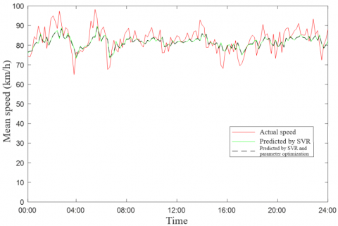
To predict the TFS without competition events, the forecast model was only provided with the TFS data on the section when no competition events took place. To fully disclose the prediction effect, the SVR forecast model was adopted to predict the time series of mean speeds in the section, respectively using the parameters obtained by the traversing method and the SA algorithm. The ratio of training data to testing data was set to 9:1. Figure 5 presents the predicted time series of mean speeds in the section.
Figure 5. The predicted mean speeds in the section without competition events
To put it more intuitively, the mean absolute percentage error (MAPE) and the root mean square error (RMSE) were selected to evaluate the forecast result. Table 1 shows the two errors of the predicted mean speeds in the section without large competition events.
Table 1. The errors of the TFS forecast without competition events
|
|
SVR |
SVR and parameter optimization |
||
|
MAPE (%) |
RMSE |
MAPE (%) |
RMSE |
|
|
Mean speed |
4.89 |
5.15 |
4.87 |
5.11 |
As shown in Figure 5 and Table 1, when no competition events took place, the SVR algorithm predicted the TFS in the section accurately, and the SA algorithm further improved the forecast accuracy by optimizing the SVR parameters. The results indicate that the parameter optimization by the SA can effectively improve the TFS forecast effect of the SVR.
4.2 Analysis on the forecast results with competition events
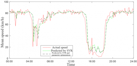
To predict the TFS with competition events, the forecast model was only provided with the TFS data on the section when competition events took place. Similarly, the SVR forecast model was employed to predict the time series of mean speeds in the section, respectively using the parameters obtained by the traversing method and the SA algorithm. The ratio of training data to testing data was set to 9:1. Figure 6 presents the predicted time series of mean speeds in the section.
Figure 6. The predicted mean speeds in the section with competition events
The MAPE and the RMSE were also selected to evaluate the forecast effect of the original SVR and our model on the TFS with competition events. Table 2 lists the two errors of the forecast results of the two models.
As can be seen in Figure 6 and Table 2, the TFS fluctuation with large competition events was much more obvious than that without large competition events, and the TFS variation was far from smooth. In this case, the forecast errors of the TFS were clearly on the rise. The MAPE soared from about 5% without competition events to around 50% with competition events. The rising error is attributable to the following factors: (1) The number of training samples is rather limited, for only a few sample data were collected on the days with competition events; (2) The short-term fluctuation of the TFS has a great impact on the forecast accuracy, which is also affected by the duration of the competition events. Despite the error increment, the SVR could predict the complete TFS trend in the section, and project the trend much more accurately after the parameters were optimized by the SA algorithm.
Table 2. The errors of the TFS forecast with competition events
|
|
SVR |
SVR and parameter optimization |
||
|
MAPE (%) |
RMSE |
MAPE (%) |
RMSE |
|
|
Mean speed |
31.46 |
10.47 |
28.44 |
10.15 |
During large competition events, the forecast of the real-time TFS in the peripheral roads can enable the competent department to take targeted traffic control measures, prevent the severe congestion caused by these events, and protect the normal and efficient operation of the road network. Therefore, this paper proposes to predict the TFS in the peripheral roads of large competition events using the SVR and parameter optimization. Firstly, the tensor recovery algorithm was adopted to fill up the missing data. Then, the SVR parameters were optimized by the SA algorithm. Next, a TFS forecast model was established based on the SVR and the optimized parameters, and verified through an example analysis. The empirical results show that our forecast model, which is based on SVR and parameter optimization, can effectively predict the real-time TFS in the peripheral roads of large competition events. Through error analysis, it is learned that the parameter optimization can greatly improve the forecast accuracy of the SVR model.
It should be noted that the TFS can be characterized by many indices. Considering the data availability, our model was verified using only one input variable, namely, the mean speed of the section. Further research may build a forecast model with multiple TFS indices. Besides, the TFS features high stochasticity and volatility. In addition to large competition events, the TFS is also greatly affected by the driver’s behavioral preference, the road conditions and the weather. To forecast the TFS more comprehensively, more influencing factors should be included into the TFS prediction, creating a multi-factor TFS forecast model.
[1] Ahmed, M.S., Cook, A.R. (1979). Analysis of freeway traffic time-series data by using Box-Jenkins techniques (No. 722).
[2] Eren, M. (2018). Forecasting of the fuzzy univariate time series by the optimal lagged regression structure determined based on the genetic algorithm. Economic Computation and Economic Cybernetics Studies and Research, 52(2): 201-215.
[3] Bikku, T. (2018). A new weighted based frequent and infrequent pattern mining method on realtime E-commerce. Ingenierie des Systemes d'Information, 23(5): 121-138. https://doi.org/10.3166/isi.23.5.121-138
[4] Huang, L., Zhou, K. (2018). Modeling and application of an embedded real-time system based on real-time colored Petri net. Journal Europeen des Systemes Automatises, 51(4-6): 333-345. https://doi.org/10.3166/jesa.51.333-345
[5] Kalman, R.E. (1960). A new approach to linear filtering and prediction problems. Journal of basic Engineering, 82(1): 35-45. https://doi.org/10.1115/1.3662552
[6] Wang, S., Hu, Y.Z. (2018). Binocular visual positioning under inhomogeneous, transforming and fluctuating media. Traitement du Signal, 35(3-4): 253-276. https://doi.org/10.3166/ts.35.253-276
[7] Wang, Y., Papageorgiou, M. (2005). Real-time freeway traffic state estimation based on extended Kalman filter: a general approach. Transportation Research Part B: Methodological, 39(2): 141-167. https://doi.org/10.1016/j.trb.2004.03.003
[8] Ye, Z., Zhang, Y., Middleton, D.R. (2006). Unscented Kalman filter method for speed estimation using single loop detector data. Transportation Research Record, 1968(1): 117-125. https://doi.org/10.1177/0361198106196800114
[9] Wang, D.H., Qu, D.Y. (1998). A study of a real-time dynamic prediction method for traffic volume. China Journal of Highway and Transport, 11: 102-107.
[10] Song, X., Gao, S., Chen, C. (2018). A novel vehicle feature extraction algorithm based on wavelet moment. Traitement Du Signal, 35(3-4): 223-242. https://doi.org/10.3166/ts.35.223-242
[11] Wang, X.Y., Wu, L., Zhang, K.W., Zhang, J.L. (2005). Traffic flow forecasting method based on wavelet non-parametric regression algorithms. Systems Engineering, 23(10): 44-47.
[12] Yuan, B., Wang, F., Bao, D. (2018). Design and application of a wavelet neural network program for evaluation of goodwill value in corporate intellectual capital. Ingenierie des Systemes d'Information, 23(5): 185-200. https://doi.org/10.3166/isi.23.5.185-200
[13] Wang, D.S., He, G.G. (2003). Summary and prospects of the study on traffic chaos. China Civil Engineering Journal, 36(1): 68-74.
[14] Dong, C.J., Shao, C.F., Li, J., Meng, M. (2011). Short-term traffic flow prediction of road network based on chaos theory. Journal of System Engineering, 26(3): 340-345.
[15] Zang, L.L., Jia, L., Yang, L.C., Liu, T. (2007). Chaotic time series model of real-time prediction of traffic flow. China Journal of Highway and Transport, 20(6): 95-99.
[16] Davis, G.A., Nihan, N.L. (1991). Nonparametric regression and short-term freeway traffic forecasting. Journal of Transportation Engineering, 117(2): 178-188. https://doi.org/10.1061/(ASCE)0733-947X(1991)117:2(178)
[17] Smith, B.L., Williams, B.M., Oswald, R.K. (2002). Comparison of parametric and nonparametric models for traffic flow forecasting. Transportation Research Part C: Emerging Technologies, 10(4): 303-321. https://doi.org/10.1016/S0968-090X(02)00009-8
[18] Clark, S. (2003). Traffic prediction using multivariate nonparametric regression. Journal of Transportation Engineering, 129(2): 161-168. https://doi.org/10.1061/(ASCE)0733-947X(2003)129:2(161)
[19] Kindzerske, M.D., Ni, D. (2007). Composite nearest neighbor nonparametric regression to improve traffic prediction. Transportation Research Record, 1993(1): 30-35. https://doi.org/10.3141/1993-05
[20] Dougherty, M.S., Cobbett, M.R. (1997). Short-term inter-urban traffic forecasts using neural networks. International Journal of Forecasting, 13(1): 21-31. https://doi.org/10.1016/S0169-2070(96)00697-8
[21] Ledoux, C. (1997). An urban traffic flow model integrating neural networks. Transportation Research Part C: Emerging Technologies, 5(5): 287-300. https://doi.org/10.1016/S0968-090X(97)00015-6
[22] Sánchez-Escalona, A.A., Góngora-Leyva, E. (2018). Artificial neural network modeling of hydrogen sulphide gas coolers ensuring extrapolation capability. Mathematical Modelling of Engineering Problems, 5(4): 348-356. https://doi.org/10.18280/mmep.050411
[23] Munoz-Guijosa, J.M., Riesco, E., Olmedo, M. (2017). Neural network and training strategy design for train drivers’ vibration dose simulation. Int J Simul Model, 16: 72-83.
[24] Ruxanda, G., Opincariu, S. (2018). Bayesian neural networks with dependent Dirichlet process priors. Application to pairs trading. Economic Computation & Economic Cybernetics Studies & Research, 52(4): 5-18.
[25] Du, C., Huang, L. (2018). Text classification research with attention-based recurrent neural networks. International Journal of Computers Communications & Control, 13(1): 50-61. https://doi.org/10.15837/ijccc.2018.1.3142
[26] Yang, Z.S., Wang, Y., Guan, Q. (2006). Short-term traffic flow prediction method based on SVM. Journal of Jilin University, 36(6): 881-884.
[27] Huang, Y.L., Meng, S.Y., Li, X.S., Fan, W.Y. (2018). A classification method for wood vibration signals of Chinese musical instruments based on GMM and SVM. Traitement du Signal, 35(2): 137-151. https://doi.org/10.3166/ts.35.137-151
[28] Park, B.B. (2002). Hybrid neuro-fuzzy application in short-term freeway traffic volume forecasting. Transportation Research Record, 1802(1): 190-196. https://doi.org/10.3141/1802-21
[29] Zheng, W., Lee, D.H., Shi, Q. (2006). Short-term freeway traffic flow prediction: Bayesian combined neural network approach. Journal of Transportation Engineering, 132(2): 114-121. https://doi.org/10.1061/(ASCE)0733-947X(2006)132:2(114)
[30] Boto‐Giralda, D., Díaz‐Pernas, F.J., González‐Ortega, D., Díez‐Higuera, J.F., Antón‐Rodríguez, M., Martínez‐Zarzuela, M., Torre‐Díez, I. (2010). Wavelet‐based denoising for traffic volume time series forecasting with self‐organizing neural networks. Computer‐Aided Civil and Infrastructure Engineering, 25(7): 530-545. https://doi.org/10.1111/j.1467-8667.2010.00668.x
[31] Zhang, N., Zhang, Y., Lu, H. (2011). Seasonal autoregressive integrated moving average and support vector machine models: Prediction of short-term traffic flow on freeways. Transportation Research Record, 2215(1): 85-92. https://doi.org/10.3141/2215-09