Hayam G. Wahdan* | Hisham E. Abdelslam | Tarek H.M. Abou-El-Enien | Sally S. Kassem
© 2020 IIETA. This article is published by IIETA and is licensed under the CC BY 4.0 license (http://creativecommons.org/licenses/by/4.0/).
OPEN ACCESS
Meta heuristic algorithms are very important methods, they used mainly in solving combinatorial optimization problems. They are stochastic in manner and simulate the behavior of any population of particles. Meta heuristics algorithms try to find optimal or near to optimal solution when solving complex optimization problem. In this paper two modified emperor penguins colony optimization algorithms MEPC1 and MEPC2 were developed. Original Emperor Penguins Colony (EPC) algorithm simulates the behavior of emperor of penguins, two modifications are done to the original EPC, Archimedes and hyperbolic spiral like movement are used instead of logarithmic spiral like movement. The two modified algorithms are compared with the original algorithm through ten test functions; the results show that the modified algorithms are achieved better than the original one.
meta heuristic, optimization, emperor penguin colony, nature inspired
Optimization is the process of finding better or optimal solution for any problem, optimization find the maximum value in case of maximization problem and minimum value in case of minimization problem. inputs of any optimization problem are sets of variables represent decision variables, constraints represent the restrictions should be considered in solving the problem and finally the target or the objective function being optimize whether maximized or minimized [1].
Meta heuristic is defined in computer science and mathematical optimization as high level strategies designed mainly to solve optimization problem, find effective and efficient solution instead of finding approximate solution, methods are approximate and often uncertain (random), it try to find optimal or near to optimal solution to the optimization problem through set of procedures. Metaheuristics solve faster complex and combinatorial optimization problem [2].
Metaheuristics can be classified into four categories according to the behavior the algorithm simulate, physical based, swarm based, evolutionary based and human based. In physical-based methods, search agents move across the search space according to the laws of physics such as electromagnetic force, displacement, inertia force, gravity, and so on. Simulating Annealing (SA) [3], Gravity Search Algorithm (GSA) [4], Big Bang Algorithm (BBA) [5], and Charged System Search (CSS) [6], are most commonly examples of physical based optimization algorithm. In evolutionary-based methods, biological evolution such as reproduction, recombination, selection, and mutation are inspired. Evolutionary based like Genetic Algorithm (GA) [7], Differential Evolutionary (DE) [8], and Imperialist Competitive Algorithm (ICA) [9]. Swarm-based methods are based on simulate the behavior of group of animal such as birds, insects, fishes and others like Particle Swarm Optimization (PSO) [10], Ant Colony (AC) [11], Bat Swarm (BS) [12], Cuckoo Search (CS) [13], and Emperor Penguins Colony (EPC) [2]. and human based it is unique nature inspired because it simulates nature phenomena commonly associated with human like Harmony Search (HC) [14], and Firework Algorithm (FA) [15].
The Emperor Penguins Colony (EPC) is one of the most recent swarm-based optimization algorithms. It provides Quick convergence; it can start the optimization process using small population size; and EPC has achieved remarkable performance in solving complex problems using one type of spiral-like movements, namely, the logarithmic spiral-like movement. Spiral-like movements may also be performed using other techniques, for example: Archimedes, parabolic and hyperbolic. Due to the noticeable performance of EPC in solving complex problems, this work is motivated to examine the efficiency of EPC in solving complex problems under different types of spiral-like movements, namely, the Archimedes and hyperbolic movements. Hence, this work develops two modified algorithms, the first modified Emperor Penguins Colony (MEPC1) utilizes Archimedes spiral like movement, and the second modified Emperor Penguins Colony (MEPC2) utilizes hyperbolic spiral-like movement. These two modified algorithms outperform, in most instances, the original EPC utilizing logarithmic spiral-like movement.
The rest of the paper is organized as follows, Section 2 provides the literature review about the swarm based methods, Section 3 describes the original Emperor Penguins Colony (EPC) algorithm, Section 4, 5 describes the two modified algorithms and section 6 includes experimental results and discussion and Section 7 represents conclusions and further work.
During the last decades several optimization algorithms have been developed, many of which are classified as swarm optimization algorithms. EPC is classified as a swarm-based optimization algorithm. Therefore, this section summarizes a number of the swarm-based optimization algorithms that are widely and usefully utilized to solve many optimization problems.
Ant Colony Optimization (ACO); developed Marco Dorigo in 1992; was Inspired by the foraging behavior of ants, ACO achieved high performance and robustness in solving combinatorial optimization problems [11]. Particle Swarm Optimization (PSO) algorithm was originally introduced by Kennedy and Eberhart in 1995. The algorithm was inspired by mimicking the social interaction and communication within a flock of birds or school of fishes, it can be applied in many applications like engineering and scientific researches and don't overlapping and mutation calculation [10]. Artificial Bee Colony (ABC) was proposed by Karaboga in 2005; it is inspired by the foraging behavior of bees, it can be successfully applied for large scale optimization problem [16]. Cuckoo Search (CS) algorithm was proposed by Yang and Deb in 2009. The algorithm imitates the behavior of cuckoo birds to explore the solution space for an optimum or near optimum solution; it is efficient in solving discrete optimization problem [13]. Bat Algorithm (BA) is proposed by Xin-She Yang in 2010, it is simple and flexible optimization algorithm [12].
Firefly Algorithm (FA) developed by Kwiecien and Filipowicz in 2010, is a useful and powerful algorithm for solving discrete and nonlinear optimization problems [17]. Lion Optimization (LO) population based optimization model developed by Rajakumar in 2012, it is simulate the behavior of lions in hunting the animals, it is succeeded to obtain optimal or near to optimal solution [18]. Chicken Swarm Optimization (CSO) algorithm developed by Liu et al. in 2014, simulates the behavior of chickens, it can achieve good optimizing results in term of accuracy and robustness [19]. Social Spider Algorithm (SSA) developed by James et al. in 2015, is powerful in solving continuous optimization problem and easy to implement [20]. Spider Monkey (SM) developed by Bansal et al. 2014, inspired by the intelligent behavior of spider monkeys when searching for food sources, it is proved its capability of solving real world complex problems that cannot solved by the classical techniques [21]. African buffalo optimization (ABO) developed by Odili et al. in 2014, was inspired by the practice of African buffalos in the vast African forests, through set of simple steps ABO can solve complex optimization problems [22]. Grasshopper optimization Algorithm (GOA) was developed by Saremi et al. in 2017, the algorithm simulates the behavior of grasshoppers' swarms in nature for solving complex optimization problem [23].
Laying chicken algorithm (LCA) is developed by Hosseini in 2017, is used to solve different types of the problems whether linear or nonlinear optimization problems [24]. Owl search algorithm (OSA) is a population based optimization algorithm, developed by Hosseini in 2018. It is based on the hunting mechanism of owls [25]. Emperor Penguin Colony (EPC) developed by Harifi et al. in 2019, simulates the behavior of penguins in their colonies when moving from low to high temperatures in spiral like movements, it is powrful in solving complex optimaztion problem [2].
A new Meta heuristics algorithm named The Emperor Penguin Colony (EPC) was proposed by Harifi et al. in 2019. The algorithm inspired by the behavior of emperor penguins in colonies when they move from a cold domain to a warmer one following a logarithmic spiral like movement, [2]. This algorithm is controlled by the body heat radiation of the penguins and their spiral-like movement in their colony. The algorithm tries to find optimal or near to optimal solution.
In the EPC, the temperature around the huddle is calculated, the algorithm is vector based equations, when the body temperature is calculated and body heat radiation of each penguin and then due to distance and attractiveness each penguin performs the spiral-like movement.
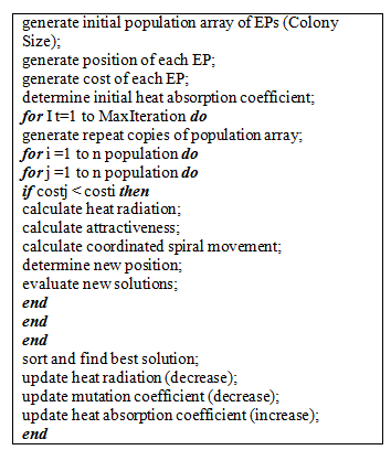
EPC starts with a set of penguins representing the population size. These penguins are distributed in nature with calculated position and cost, penguins are continually moving in the direction of low objective value penguins, these penguins with high intensity. The objective function value is calculated using heat intensity and the distance. Attraction is done, a new solution is evaluated and the heat intensity is updated. All solutions are sorted and the best is selected. Damping ratio for heat radiation, movement, and heat absorption is applied. Figure 1 describes pseudo code of the EPC algorithm.
This algorithm is performed according to the following rules [2]:
1- All penguins in the initial population have heat radiation and attract to each other due to absorption coefficient.
2- The body surface area of all penguins is considered equal to each other.
3- Penguin absorbs the full heat radiation and the effect of the earth’s surface and the atmosphere are not regarded.
4- The heat radiation of penguins is considered linear.
5- The attraction of penguin is done according to the amount of heat in the distance between two penguins.
6- The penguin spiral movement during the absorption process is not monotonous and has a deviation with uniform distribution.
Figure 1. pseudo code of the EPC algorithm, [2]
The heat radiation of each penguin is calculated using Eq. (1),
$Q_{\text {penguin}}=A \mathcal{E} \sigma T_{s}^{4}$ (1)
where, Qpenguin is heat transfer per unit of time, A is total surface area of the penguin which equal to 0.56 m2. Ɛ is emissivity of bird plumage which is considered 0.98, σ is the Stefan–Boltzmann constant (5.6703×10⁻⁸ W/m2K4) and Ts is the absolute temperature in Kelvin (K) which is considered 35℃ equal to 308.15 K [2].
The attractiveness Q is calculated using Eq. (2)
$Q=A \varepsilon \sigma T_{S}^{4} e^{-\mu x}$ (2)
where, μ is attenuation coefficient and x is the distance between two linear sources.
The calculation of the coordinated spiral movement and the new position is done using logarithmic spiral movement in the original EPC [2]. The following sections present the 2 modifications proposed by this work, namely Archimedes and hyperbolic spiral like movement for calculating the coordinated spiral movement and new positions of penguins, equations 3 till equation 10 provide full explanation about the calculation of coordinated spiral movement and the new position.
The EPC algorithm has set of advantages , it is using spiral like movement to optimize temperature without need to determine the boundary of the huddle; Quick convergence; it can start the optimization process using small population size; Not limited to monotonous spiral path; and it provides acceptable performance to solve high-dimensional problems.
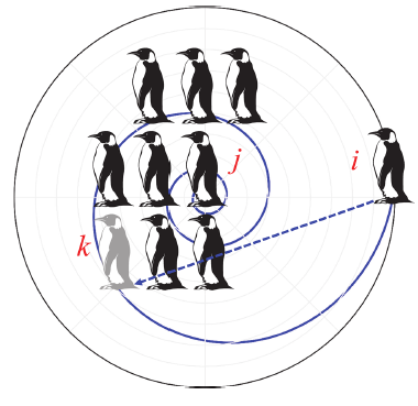
The penguins start spiral-like huddle in which the clockwise movement is done around a constant center as shown in Figure 2. In this case, the structure of the system has uncertain boundaries with a spiral pattern around the center. The warmest temperature is at the center of the huddle and gets colder as we move towards the perimeter.
As shown in Figure 2, there are two penguins i and j, these penguins move from low temperature position, represented by position i, to a higher temperature position, represented by position j. The movement from position i to position j is a spiral like movement. There are many types of spiral like movements, for example: logarithmic, Archimedes, parabolic and hyperbolic. The original EPC assumes logarithmic spiral like movement.
In the First modification proposed by this work, the Emperor Penguins Colony (MEPC1) algorithm considers Archimedes spiral like movement. Archimedes spiral like movement considers a relation between r and θ as shown in Eq. (3),
$r=a \theta$ (3)
where, θ is the angle of the x-axis, a is a constant and r represents the distance from the origin.
As shown in Figure 2, the penguin i is attracted into j and starts the spiral-like movement. To obtain the equation of this spiral-like movement, first the distance between two penguins i and j must be calculated according to Eq. (4). Eq. (4) represents the distance between i and j but we have attractiveness Q. The Q is a coefficient of spiral-like movement. For simple example if the distance between i and j is equal to 2 and Q is equal to 0.8, we have 0.8*2=1.6 which 1.6 is distance traveled to point k.
Figure 2. Spiral like movement of emperor penguins
The distance between penguins i and j (Dij) is represent by the arc length from i to j, which is calculated according to Eq. (4),
$D_{i j}=\int_{\theta i}^{\theta j} \sqrt{\left(\frac{d r}{d \theta}\right)^{2}+r^{2} d \theta}=\frac{a}{2}\left(\left(\theta_{j} \sqrt{1+\theta_{j}^{2}}+\sinh ^{-1}\left(\theta_{j}\right)-\left(\theta_{i} \sqrt{1+\theta_{i}^{2}}+\sinh ^{-1}\left(\theta_{i}\right)\right)\right.\right.$ (4)
and
$D_{i k}=\frac{a}{2}\left(\left(\theta_{k} \sqrt{1+\theta_{k}^{2}}+\sinh ^{-1}\left(\theta_{k}\right)-\left(\theta_{i} \sqrt{1+\theta_{i}^{2}}+\sinh ^{-1}\left(\theta_{i}\right)\right)\right.\right.$ (5)
To find the value of θk in terms of θi and θj, we using the relation between Dik and Dij this relation represented in Eq. (6). This relation declare that distance traveled from i to k equal the attractiveness Q times the distance form i to j,
$D_{i k}=Q * D_{i j}$ (6)
$\left(\theta_{k} \sqrt{1+\theta_{k}^{2}}+\sinh ^{-1}\left(\theta_{k}\right)=Q\left(\theta_{j} \sqrt{1+\theta_{j}^{2}}+\sinh ^{-1}\left(\theta_{j}\right)\right)-(1-Q)\left(\theta_{i} \sqrt{1+\theta_{i}^{2}}+\sinh ^{-1}\left(\theta_{i}\right)\right)\right.$ (7)
To find the value of θk numerical solution is done to Eq. (7) using (nsolve) function in matlab, nsolve function aims to find numerical approximations to the solutions of the system of equations or inequalities, after finding the value of θk, the x and y components of the position k are obtained in terms of the components x and y of points i, j, and attractiveness Q. coordinates of the new position k can be calculated using the following Eqns. (8)-(9),
$x_{k}=r \cos \theta_{k},$ since $r=a \theta \operatorname{so~} x_{k}=a \theta_{k} \cos \theta_{k}$ (8)
$y_{k}=r \sin \theta_{k},$ since $r=a \theta$ so $y_{k}=a \theta_{k} \sin \theta_{k}$ (9)
Accordingly, penguin i will move spirally then it’s summed with a random vector and is transported to a new position as shown in Eqns. (10) and (11).
$x_{k}=a \theta_{k} \cos \theta_{k}+\phi \varepsilon_{i}$ (10)
$y_{k}=a \theta_{k} \sin \theta_{k}+\phi \varepsilon_{i}$ (11)
where, ф is the mutation factor in the change of path and Ɛi is a random vector. This random vector $\epsilon$ can be any distribution like Uniform, Normal or Lévy distribution. In these algorithms a Uniform distribution is assumed. The function of this equation is exactly the same as the function of a mutation, which is performed after the crossover in the GA algorithm.
In the second modification to the Emperor Penguins Colony (MEPC2), the hyperbolic spiral like movement algorithm is assumed. Hyperbolic spiral like movement considers a relation between r and θ as shown in Eq. (12),
$r=\frac{a}{\theta}$ (12)
where, θ is the angle of the x-axis, a is a constant and r shows the distance from the origin.
The distance between penguins i and j is calculated according to Eq. (13),
$D_{i j}=\int_{\theta i}^{\theta j} \sqrt{\left(\frac{d r}{d \theta}\right)^{2}+r^{2} d \theta}=a\left(-\frac{\sqrt{1+\theta_{j}^{2}}}{\theta_{j}}+\ln \left(\theta_{j+} \sqrt{1+\theta_{j}^{2}}\right)-\left(-\frac{\sqrt{1+\theta_{i}^{2}}}{\theta_{i}}+\ln \left(\theta_{i+} \sqrt{1+\theta_{i}^{2}}\right)\right)\right)$ (13)
and
$D_{i k}=a\left(\left(-\frac{\sqrt{1+\theta_{k}^{2}}}{\theta_{k}}+\ln \left(\theta_{k+\sqrt{1+\theta_{k}}^{2}}\right)\right)-\left(-\frac{\sqrt{1+\theta_{i}^{2}}}{\theta_{i}}+\ln \left(\theta_{i+\sqrt{1+\theta_{i}^{2}}}\right)\right)\right)$ (14)
Thus,
$\left(-\frac{\sqrt{1+\theta_{k}^{2}}}{\theta_{k}}+\ln \left(\theta_{k+} \sqrt{1+\theta_{k}^{2}}\right)\right)=Q\left(\ln \left(\theta_{j+} \sqrt{1+\theta_{j}^{2}}\right)-\frac{\sqrt{1+\theta_{j}^{2}}}{\theta_{j}}\right)-(1-Q)\left(\ln \left(\theta_{i+} \sqrt{1+\theta_{i}^{2}}\right)-\frac{\sqrt{1+\theta_{i}^{2}}}{\theta_{i}}\right)$ (15)
To find the value of θk in term of θi and θj numerical solution is done to Eq. (15) using (nsolve) function in matlab, nsolve function aims to find numerical approximations to the solutions of the system of equations or inequalities, after finding the value of θk, the x and y components of the position k are obtained in terms of the components x and y of points i, j, and attractiveness Q. coordinates of the new position k can be calculated using the following Eqns. (16)-(17),
$x_{k}=r \cos \theta_{k},$ since $r=\frac{a}{\theta}$ so $x_{k}=\frac{a}{\theta} \cos \theta_{k}$ (16)
$y_{k}=r \sin \theta_{k}, \operatorname{sincer}=\frac{a}{\theta}$ so $y_{k}=\frac{a}{\theta} \sin \theta_{k}$ (17)
In this way, the penguin i will move spirally then it’s summed with a random vector and is transported to a new position as shown in Eqns. (18) and (19).
$x_{k}=\frac{a}{\theta} \cos \theta_{k}+\phi \varepsilon \mathrm{i}$ (18)
$y_{k}=\frac{a}{\theta} \sin \theta_{k}+\phi \varepsilon i$ (19)
where, ф is the mutation factor in the change of path and Ɛi is a random vector.
6.1 Benchmark function
Ten test functions are used to evaluate the performance, accuracy and the convergence of the algorithm. These test function detailed explained in this web site http://www.sfu.ca/~ssurjano/.
6.2 Comparison between algorithms
In this section a set of comparisons are conducted. First a comparison between the original EPC, first modified EPC (MEPC1), and second modified EPC (MEPC2) are provided. Another comparison is conducted between MEPC1 and MEPC2 against Genetic Algorithm (GA) [7], Imperialist Competitive Algorithm (ICA) [9], Particle Swarm Optimization (PSO) [10], Artificial Bee Colony (ABC) [26], Differential Equation (DE) [8], Harmony Search (HS) [14], Invasive Weed Optimization (IWO) [27], Grey Wolf Optimizer (GWO) [28], and Cuckoo search (CS) [29]. The last comparison aims to investigate the performance of the two proposed modified algorithms against other algorithms available in the literature.
Parameters of MEPC1 and MEPC2 are set as follows: the maximum number of iterations is 100, the penguins population size is 20, the number of decision variables equal 5. Each algorithm was run 30 times, with 100 iterations per run. So the mean and stander derivation of 30 runs was considered,
Table 1 provides a comparison between the original EPC and MEPC1. Values recorded in Table 1 regarding MEPC1 are mean objective function values of 30 runs. Table 1 shows that MEPC1 is able to achieve 70% improvement over the original EPC, where seven problems out of 10 record better mean objective function values.
Table 2 provides a comparison between the original EPC and MEPC2. Values recorded in Table 2 regarding MEPC2 are mean objective function values of 30 runs. Table 2 shows that MEPC2 is able to achieve 80% improvement over the original EPC, where eight problems out of 10 record better mean objective function values.
Table 1. Mean of 30 runs between EPC and MEPC1
|
Functions |
MEPC1 |
EPC |
|
Ackly |
8.88E-16 |
3.18E-08 |
|
Sphere |
1.17E-44 |
3.32E-16 |
|
Rosenbrock |
3.83E+00 |
3.8752 |
|
Rastrigin |
0 |
5.80E-14 |
|
Griewank |
0 |
1.31E-02 |
|
Bukin |
0.1 |
9.56E-02 |
|
Bohachevsky |
0 |
1.11E-17 |
|
Zakharov |
2.54E-44 |
5.49E-16 |
|
Booth |
50.129699 |
7.34E-18 |
|
Michalewicz |
-5.52E-13 |
-1.80E+00 |
Table 2. Mean of 30 runs between EPC and MEPC2
|
Functions |
MEPC2 |
EPC |
|
Ackly |
8.88E-16 |
3.18E-08 |
|
Sphere |
3.28E-36 |
3.32E-16 |
|
Rosenbrock |
0.003863 |
3.8752 |
|
Rastrigin |
0 |
5.80E-14 |
|
Griewank |
0 |
1.31E-02 |
|
Bukin |
0.1 |
9.56E-02 |
|
Bohachevsky |
0 |
1.11E-17 |
|
Zakharov |
5.77E-35 |
5.49E-16 |
|
Booth |
1.954526 |
7.34E-18 |
|
Michalewicz |
-2.32001 |
-1.80E+00 |
Table 3. St-dev of 30 runs between EPC and MEPC1
|
Functions |
EPC |
MEPC1 |
MEPC2 |
|
Ackly |
6.78E-09 |
1.01043E-31 |
2.00587E-31 |
|
Sphere |
1.36E-16 |
4.74949E-44 |
4.85506E-36 |
|
Rosenbrock |
0.0435 |
0.311715323 |
0.008073997 |
|
Rastrigin |
2.58E-14 |
0 |
0 |
|
Griewank |
0.0118 |
0 |
0 |
|
Bukin |
0.025 |
3.79049E-10 |
3.79049E-10 |
|
Bohachevsky |
4.47E-17 |
0 |
0 |
|
Zakharov |
1.82E-16 |
9.67701E-44 |
1.41975E-34 |
|
Booth |
6.47E-18 |
1.353043223 |
0.157821921 |
|
Michalewicz |
0.2612 |
4.12634E-13 |
0.274268392 |
Table 4 provides comparison between MEPC1, MEPC2 and GA. The results obtained declare that MEPC1 achieves better in 70% of the tested function, GA performs better in three test function Rosenbrock, booth and Michalewicz. MEPC2 achieves better in 80% of the tested function, GA perform better in two test function booth and Michalewicz. GA achieves better in these test function may be the nature of these problems, being nonlinear, non-convex and multimodal.Table 3 provides the standard deviation of 30 runs of the three Algorithms, EPC, MEPC1, and MEPC2. Standard deviation is used to assess how far the values are spread above and below the mean. Algorithms with low values of standard deviation tend to be more reliable than those with higher standard deviation values. We notice that the two modified algorithms provide more reliable results.
As shown in Table 5, MEPC1 does better in 60% of test functions, while ICA does better in four test functions (Rosenbrock, Bukin, booth and Michalewicz); MEPC2 does better in 70% of test functions, while ICA does better in three test functions (Bukin, booth and Michalewicz). The excellence of ICA is the result of the nonlinear, non-convex, and multimodal nature of the problems.
Table 6 provides comparison between MEPC1, MEPC2 and PSO. The results obtained declare that MEPC1 achieves better in 70% of the tested function, PSO performs better in three test functions Rosenbrock, Booth and Michalewicz. MEPC2 achieves better in 80% of the tested function, PSO performs better in two test functions Booth and Michalewicz. PSO achieves better in these test function may be the nature of these problems, being nonlinear, non-convex and multimodal.
Table 7 provides comparison between MEPC1, MEPC2 and ABC. The results obtained declare that MEPC1 achieves better in 80% of the tested function, ABC performs better in two test functions Booth and Michalewicz. MEPC2 achieves better in 80% of the tested function, ABC performs better in two test functions Booth and Michalewicz. ABC achieves better in these test function may be the nature of these problems, being nonlinear, non-convex and multimodal.
Table 4. Comparison between MEPC1, MEPC2 and GA
|
Functions |
MEPC1 |
MEPC2 |
GA |
|
Ackly |
8.88E-16 |
8.88E-16 |
0.0907 |
|
Sphere |
1.17E-44 |
3.28E-36 |
0.0028 |
|
Rosenbrock |
3.825285 |
0.003863 |
2.6338 |
|
Rastrigin |
0 |
0 |
0.9373 |
|
Griewank |
0 |
0 |
0.0437 |
|
Bukin |
0.1 |
0.1 |
1.1704 |
|
Bohachevsky |
0 |
0 |
0.0085 |
|
Zakharov |
2.54E-44 |
5.77E-35 |
2.2252 |
|
Booth |
50.1297 |
1.954526 |
0.0582 |
|
Michalewicz |
-5.5E-13 |
-2.32001 |
-4.5633 |
Table 5. Comparison between MEPC1, MEPC2 and ICA
|
Functions |
MEPC1 |
MEPC2 |
ICA |
|
Ackly |
8.88E-16 |
8.88E-16 |
2.63E-04 |
|
Sphere |
1.17E-44 |
3.28E-36 |
4.95E-06 |
|
Rosenbrock |
3.825285 |
0.003863 |
3.3888 |
|
Rastrigin |
0 |
0 |
1.2083 |
|
Griewank |
0 |
0 |
0.0264 |
|
Bukin |
0.1 |
0.1 |
0.0759 |
|
Bohachevsky |
0 |
0 |
3.64E-13 |
|
Zakharov |
2.54E-44 |
5.77E-35 |
0.3906 |
|
Booth |
50.1297 |
1.954526 |
0.0028 |
|
Michalewicz |
-5.5E-13 |
-2.32001 |
-4.5706 |
Table 6. Comparison between MEPC1, MEPC2 and PSO
|
Functions |
MEPC1 |
MEPC2 |
PSO |
|
Ackly |
8.88E-16 |
8.88E-16 |
6.09E-04 |
|
Sphere |
1.17E-44 |
3.28E-36 |
9.04E-08 |
|
Rosenbrock |
3.825285 |
0.003863 |
1.7793 |
|
Rastrigin |
0 |
0 |
2.9004 |
|
Griewank |
0 |
0 |
0.0222 |
|
Bukin |
0.1 |
0.1 |
0.2298 |
|
Bohachevsky |
0 |
0 |
4.70E-10 |
|
Zakharov |
2.54E-44 |
5.77E-35 |
4.70E-06 |
|
Booth |
50.1297 |
1.954526 |
8.49E-11 |
|
Michalewicz |
-5.5E-13 |
-2.32001 |
-4.12E+00 |
Table 7. Comparison between MEPC1, MEPC2 and ABC
|
Functions |
MEPC1 |
MEPC2 |
ABC |
|
Ackly |
8.88E-16 |
8.88E-16 |
0.1421 |
|
Sphere |
1.17E-44 |
3.28E-36 |
0.0102 |
|
Rosenbrock |
3.825285 |
0.003863 |
15.4923 |
|
Rastrigin |
0 |
0 |
10.7627 |
|
Griewank |
0 |
0 |
0.1333 |
|
Bukin |
0.1 |
0.1 |
0.7341 |
|
Bohachevsky |
0 |
0 |
3.01E-07 |
|
Zakharov |
2.54E-44 |
5.77E-35 |
3.9614 |
|
Booth |
50.1297 |
1.954526 |
8.10E-06 |
|
Michalewicz |
-5.5E-13 |
-2.32001 |
-2.8306 |
Table 8. Comparison between MEPC1, MEPC2 and DE
|
Functions |
MEPC1 |
MEPC2 |
DE |
|
Ackly |
8.88E-16 |
8.88E-16 |
1.77E-04 |
|
Sphere |
1.17E-44 |
3.28E-36 |
1.34E-08 |
|
Rosenbrock |
3.825285 |
0.003863 |
1.9891 |
|
Rastrigin |
0 |
0 |
0.2993 |
|
Griewank |
0 |
0 |
0.0139 |
|
Bukin |
0.1 |
0.1 |
0.8872 |
|
Bohachevsky |
0 |
0 |
8.45E-13 |
|
Zakharov |
2.54E-44 |
5.77E-35 |
0.183 |
|
Booth |
50.1297 |
1.954526 |
2.80E-05 |
|
Michalewicz |
-5.5E-13 |
-2.32001 |
-4.7952 |
Table 9. Comparison between MEPC1, MEPC2 and HS
|
Functions |
MEPC1 |
MEPC2 |
HS |
|
Ackly |
8.88E-16 |
8.88E-16 |
2.0935 |
|
Sphere |
1.17E-44 |
3.28E-36 |
0.4327 |
|
Rosenbrock |
3.825285 |
0.003863 |
69.4738 |
|
Rastrigin |
0 |
0 |
7.3835 |
|
Griewank |
0 |
0 |
0.0444 |
|
Bukin |
0.1 |
0.1 |
1.9679 |
|
Bohachevsky |
0 |
0 |
0.0056 |
|
Zakharov |
2.54E-44 |
5.77E-35 |
4.4355 |
|
Booth |
50.1297 |
1.954526 |
0.016 |
|
Michalewicz |
-5.5E-13 |
-2.32001 |
-4.4896 |
Table 8 provides comparison between MEPC1, MEPC2 and DE. The results obtained declare that MEPC1 achieves better in 70% of the tested function, DE performs better in three test functions Rosenbrock, Booth and Michalewicz. MEPC2 achieves better in 80% of the tested function, DE performs better in two test functions Booth and Michalewicz. DE achieves better in these test function may be the nature of these problems, being nonlinear, non-convex and multimodal.
Table 9 provides comparison between MEPC1, MEPC2 and HS. The results obtained declare that MEPC1 achieves better in 80 % of the tested function, HS performs better in two test functions Booth and Michalewicz. MEPC2 achieves better in 80% of the tested function, HS performs better in two test functions Booth and Michalewicz. HS achieves better in these test function may be the nature of these problems, being nonlinear, non-convex and multimodal.
Table 10 provides comparison between MEPC1, MEPC2 and IWO. The results obtained declare that MEPC1 achieves better in 80% of the tested function, IWO performs better in two test functions Rosenbrock, Booth and Michalewicz. MEPC2 achieves better in 80% of the tested function, IWO performs better in two test functions Booth and Michalewicz. IWO achieves better in these test function may be the nature of these problems, being nonlinear, non-convex and multimodal.
Table 11 provides comparison between MEPC1, MEPC2 and GWO. The results obtained declare that MEPC1 achieves better in 70% of the tested function, GWO performs better in three test functions Rosenbrock, Booth and Michalewicz. MEPC2 achieves better in 90% of the tested function, GWO performs better in one test functions Michalewicz. GWO achieves better in this test function may be the nature of these problems, being nonlinear and multimodal.
Table 12 provides comparison between MEPC1, MEPC2 and CS. The results obtained declare that MEPC1 achieves better in 70% of the tested function, CS performs better in three test functions Bukin, Booth and Michalewicz. MEPC2 achieves better in 70% of the tested function, CS performs better in three test functions Bukin, Booth and Michalewicz. CS achieves better in these test function may be the nature of these problems, being nonlinear, non-convex and multimodal.
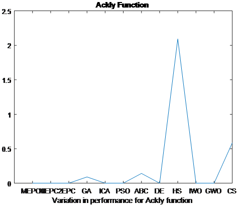
Another analysis was conducted, it provides the variation of each test function though the eleven Meta heuristics, the x- axis provides the eleven Meta heuristics algorithms, while y-axis provides the objective function value. Figure 3 provides the variation in performance of Ackley test function over eleven Meta heuristics algorithms, however the Ackley function has several local minima, the best answer is obtained by MEPC1 and MEPC2 algorithms, this best answer which represent the minimum objective function value.
Table 10. Comparison between MEPC1, MEPC2 and IWO
|
Functions |
MEPC1 |
MEPC2 |
IWO |
|
Ackly |
8.88E-16 |
8.88E-16 |
0.0019 |
|
Sphere |
1.17E-44 |
3.28E-36 |
9.21E-07 |
|
Rosenbrock |
3.825285 |
0.003863 |
9.4521 |
|
Rastrigin |
0 |
0 |
14.9577 |
|
Griewank |
0 |
0 |
0.0435 |
|
Bukin |
0.1 |
0.1 |
0.2859 |
|
Bohachevsky |
0 |
0 |
2.00E-07 |
|
Zakharov |
2.54E-44 |
5.77E-35 |
2.49E-06 |
|
Booth |
50.1297 |
1.954526 |
2.76E-08 |
|
Michalewicz |
-5.5E-13 |
-2.32001 |
-3.94E+00 |
Table 11. Comparison between MEPC1, MEPC2 and GWO
|
Functions |
MEPC1 |
MEPC2 |
GWO |
|
Ackly |
8.88E-16 |
8.88E-16 |
1.92E-05 |
|
Sphere |
1.17E-44 |
3.28E-36 |
2.76E-12 |
|
Rosenbrock |
3.825285 |
0.003863 |
1.7491 |
|
Rastrigin |
0 |
0 |
2.6374 |
|
Griewank |
0 |
0 |
0.0542 |
|
Bukin |
0.1 |
0.1 |
0.1509 |
|
Bohachevsky |
0 |
0 |
7.18E-08 |
|
Zakharov |
2.54E-44 |
5.77E-35 |
1.69E-08 |
|
Booth |
50.1297 |
1.954526 |
1.9738 |
|
Michalewicz |
-5.5E-13 |
-2.32001 |
-2.4935 |
Table 12. Comparison between MEPC1, MEPC2 and CS
|
Functions |
MEPC1 |
MEPC2 |
CS |
|
Ackly |
8.88E-16 |
8.88E-16 |
5.84E-01 |
|
Sphere |
1.17E-44 |
3.28E-36 |
4.51E-10 |
|
Rosenbrock |
3.825285 |
0.003863 |
2.53E+01 |
|
Rastrigin |
0 |
0 |
5.44E+01 |
|
Griewank |
0 |
0 |
4.41E-04 |
|
Bukin |
0.1 |
0.1 |
0.0036 |
|
Bohachevsky |
0 |
0 |
9.2174 |
|
Zakharov |
2.54E-44 |
5.77E-35 |
2.30E+02 |
|
Booth |
50.1297 |
1.954526 |
3.21E-09 |
|
Michalewicz |
-5.5E-13 |
-2.32001 |
-8.9059 |
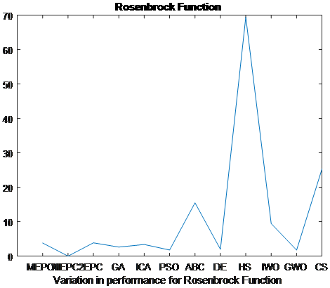
Figure 4 provides the variation in performance of Sphere test function, sphere is a simple function without local minima, MEPC1 algorithm provides the minimum objective function value comparing to the remaining Meta heuristics. Figure 5 provides the variation in performance of the Rosenbrock test function, MEPC2 provides the minimum objective function value comparing to the remaining Meta heuristics.
Figure 3. Variation in performance for Ackly Function
Figure 6 provides variation in performance of the Rastrigin test function, although Rastrigin has several local minima, the best answer is obtained by the MEPC1 and MEPC2 algorithms. Figure 7 provides variation in performance of Griewank test function, Griewank has several local minima, and the best answer is obtained by MEPC1 and MEPC2 algorithms.
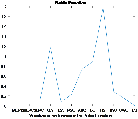
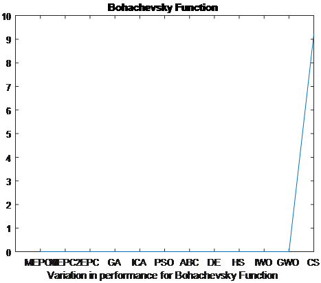
Figure 8 provides the variation in performance of Bukin test function, Bukin function has many local minima, CS provides the minimum objective function value comparing to the remaining Meta heuristics. Figure 9 provides the variation in performance of the Bohachevsky test function, MEPC1 and MEPC2 algorithms provide the best results comparing to the remaining Meta heuristics.
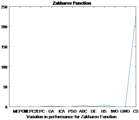
Figure 10 provides the variation in performance of Zakharov test function, Although the Zakharov is a function without a local minima, MEPC1 provides the minimum objective function value comparing to the remaining Meta heuristic. Figure 11 provides the variation in performance of Booth test function. EPC provides the minimum objective function value comparing to the remaining Meta heuristics.
Figure 4. Variation in performance for Sphere Function
Figure 5. Variation in performance for Rosenbrock Function
Figure 6. Variation in performance for Rastrigin Function
Figure 7. Variation in performance for Griewank Function
Figure 8. Variation in performance for Bukin Function
Figure 9. Variation in performance for Bohachevsky Function
Figure 10. Variation in performance for Zakharov Function
Figure 11. Variation in performance for Booth Function
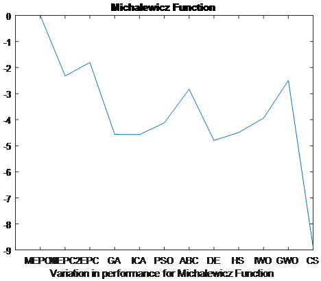
Figure 12. Variation in performance for Michalewicz Function
And finally Figure 12 provides the variation in performance of Michalewicz test function, The Michalewicz function is a multi-modal and complex function CS provides the minimum objective function value comparing to the remaining Meta heuristics.
We can conclude from all the above, after set of experiments, the two proposed algorithms MEPC1 and MEPC2 achieve best solutions in most cases. But under complex nature of the problem, complex conditions of the problem and without the existence the local minima, the proposed algorithms not achieve better. The proposed algorithms mainly not proceed better in two test functions, Booth and Michalewicz due to the complex nature of these problems.
More runs are conducted to check the behaviour with regards to changes in the parameter ф, the changes of the values of mutation factor don't much affected the results obtained. We changed the value of mutation from 0.01 till 0.09 and the results not much changed, we used 0.05 times range (max-min) as preferred in literature.
The original EPC algorithm is swarm based and nature inspired that controlled by the thermal radiation and spiral like movement of penguins, it uses logarithmic spiral like movement of penguins. In this research we developed two modified algorithms named MEPC1 and MEPC2. These two modified algorithms are based mainly on the change of the spiral like movement. MEPC1 algorithm uses Archimedes spiral like movement, and MEPC2 algorithm uses hyperbolic spiral like movement. Ten widely common benchmarks problems are used to measure the performance of the developed algorithms. MEPC1 and MEPC2 algorithms achieved better solution in most solved problems. MEPC1 achieved better in 70% of the tested function. MEPC2 achieved better in 80% of the tested functions, MEPC1 and MEPC2 also are compared to eight Meta heuristics, results declared that MEPC1 and MEPC2 achieve better in most cases. In the future, try to use EPC and the two modified algorithms in solving discrete optimization problem, solving clustering problem and complex network problems, and set of analysis can be done to test the change of the random vector $\epsilon$ from uniform to another distribution.
[1] Li, X., Yin, M. (2015). Modified cuckoo search algorithm with self-adaptive parameter method. Information Sciences, 298: 80-97. https://doi.org/10.1016/j.ins.2014.11.042
[2] Harifi, S., Khalilian, M., Mohammadzadeh, J., Ebrahimnejad, S. (2019). Emperor Penguins Colony: A new metaheuristic algorithm. Evolutionary Intelligence, 12(2): 211-226. https://doi.org/10.1007/s12065-019-00212-x
[3] Kirkpatrick, S., Gerlatt, C.D., Vecchi, M.P. (1983). Optimization by simulated annealing. Science, 220(4598): 671-680. https://doi.org/10.1126/science.220.4598.671
[4] Rashedi, E., Nezamabadi-pour, H., Saryazdi, S. (2009). GSA: A gravitational search algorithm. Information Sciences, 179(13): 2232-2248. http://dx.doi.org/10.1016/j.ins.2009.03.004
[5] Hosseini, E. (2017). Big Bang Algorithm: A new meta-heuristic approach for solving optimization problems. Asian Journal of Applied Sciences, 10(3): 134-144. http://dx.doi.org/10.3923/ajaps.2017.134.144
[6] Ahmadi, H. (2014). Charged System Search Algorithm. In Innovative Computational Intelligence: A Rough Guide to 134 Clever Algorithms. http://doi.org/10.1007/978-3-319-03404-1_20
[7] Sivanandam, S., Deepa, S. (2007). Introduction to Genetic Algorithms. Berlin: Springer Science & Business Media. https://doi.org/10.1007/978-3-540-73190-0
[8] Rainer, S., Price, K. (1997). Differential evolution–a simple and efficient heuristic for global optimization over continuous spaces. Journal of Global Optimization, 11(4): 341-359. https://doi.org/10.1023/A:1008202821328
[9] Atashpaz-Gargari, E., Lucas, C. (2007). Imperialist competitive algorithm: An algorithm for optimization inspired by imperialistic. 2007 IEEE Congress on Evolutionary Computation, Singapore, pp. 4661-4667. https://doi.org/10.1109/CEC.2007.4425083
[10] Kennedy, J. (2011). Particle swarm optimization. In Encyclopedia of machine learning and data mining. Sammut, C., Webb, G.I. (eds) Encyclopedia of Machine Learning. Springer, Boston, MA, pp. 760-766. https://doi.org/10.1007/978-0-387-30164-8_630
[11] Dorigo, M., Birattari, M., Stutzle, T. (2006). Ant colony optimization. IEEE Computational Intelligence Magazine, 1(4): 28-39. https://doi.org/10.1109/MCI.2006.329691
[12] Yang, X. (2010). A new metaheuristic bat-inspired algorithm. Nature Inspired Cooperative Strategies for Optimization (NISCO 2010), 284: 65-74. https://doi.org/10.1007/978-3-642-12538-6_6
[13] Yang, X.S., Deb, S. (2010). Engineering optimisation by Cuckoo search. Int. J. Mathematical Modelling and Numerical Optimisation, 1(4): 330-343. https://arxiv.org/abs/1005.2908
[14] Geem, Z., Kim, J., Loganathan, G. (2001). A new heuristic optimization algorithm: Harmony search. Simulation, 76(2): 60-68. https://doi.org/10.1177/003754970107600201
[15] Jain, M., Singh, V., Rani, A. (2019). A novel nature-inspired algorithm for optimization: Squirrel search algorithm. Swarm and Evolutionary Computation, 44: 148-175. https://doi.org/10.1016/j.swevo.2018.02.013
[16] Karaboga, D., Basturk, B. (2007). A powerful and efficient algorithm for numerical function optimization: artificial bee colony (ABC) algorithm. Journal of Global Optimization, 39(3): 459-471. https://doi.org/10.1007/s10898-007-9149-x
[17] Kwiecien, J., Filipowicz, B. (2012). Firefly algorithm in optimization of queueing systems. Bulletin of the Polish Academy of Sciences: Technical Sciences, 60(2): 363-368. https://doi.org/10.2478/v10175-012-0049-y
[18] Rajakumar, B. (2012). The lion's algorithm: A new nature-inspired search algorithm. Procedia Technology, 6: 126-135. https://doi.org/10.1016/j.protcy.2012.10.016
[19] Liu, Y., Meng, X., Gao, X., Zhang, H. (2014). A new bio-inspired algorithm: Chicken swarm optimization. Advances in Swarm Intelligence, 8794: 86-94. https://doi.org/10.1007/978-3-319-11857-4_10
[20] Yu, J., Li, V. (2015). A social spider algorithm for global optimization. Applied Soft Computing, 30: 614-627. https://doi.org/10.1016/j.asoc.2015.02.014
[21] Bansal, J., Sharma, H., Jadon, S., Clerc, M. (2014). Spider monkey optimization algorithm for numerical optimization. Memetic Computing, 6(1): 31-47. https://doi.org/10.1007/s12293-013-0128-0
[22] Odili, J., Kahar, M., Anwar, S. (2015). African buffalo optimization: A swarm-intelligence technique. Procedia Computer Science, 76: 443-448. https://doi.org/10.1016/j.procs.2015.12.291
[23] Saremi, S., Mirjalili, S., Lewis, A. (2017). Grasshopper Optimisation Algorithm: Theory and application. Advances in Engineering Software, 105: 30-47. https://doi.org/10.1016/j.advengsoft.2017.01.004
[24] Hosseini, E. (2017). Laying chicken algorithm: A new meta-heuristic approach to solve continuous programming problems. Journal of Applied and Computational Mathematics, 6(1): 1-8. https://doi.org/10.4172/2168-9679.1000344
[25] IJain, M., Maurya, S., Rani, A., Singh, V. (2018). Owl search algorithm: A novel nature-inspired heuristic paradigm for global optimization. Journal of Intelligent & Fuzzy Systems, 34(3): 1573-1582. https://doi.org/10.3233/JIFS-169452
[26] Karaboga, D., Basturk, B. (2007). A powerful and efficient algorithm for numerical function optimization: artificial bee colony (ABC) algorithm. Global Optim, 39(3): 459-471. https://doi.org/10.1007/s10898-007-9149-x
[27] Mehrabian, A., Lucas, C. (2006). A novel numerical optimization algorithm inspired from weed colonization. Ecological Informatics, 1(4): 355-366. https://doi.org/10.1016/j.ecoinf.2006.07.003
[28] Mirjalili, S., Mirjalili, S.M., Lewis, A. (2014). Grey wolf optimizer. Advances in Engineering Software, 69: 46-61. https://doi.org/10.1016/j.advengsoft.2013.12.007
[29] Kamoona, A., Stojcevsk, A., Patra, J.C. (2018). An enhanced cuckoo search algorithm for solving optimization problems. 2018 IEEE Congress on Evolutionary Computation (CEC), pp. 1-6. https://doi.org/10.1109/CEC.2018.8477784