Mohammad H. Mirhashemi* | Reza Anvari | Morteza Barari | Nasser Mozayani
© 2020 IIETA. This article is published by IIETA and is licensed under the CC BY 4.0 license (http://creativecommons.org/licenses/by/4.0/).
OPEN ACCESS
The use of classification methods in real-world problems has costs that are usually neglected in the early algorithms which cause inefficiencies in practice. One of these costs, which is significant in many cases, is the cost of obtaining feature values for each instance, named Test-Cost. The Ensemble of classifiers as a common and practical classification method, is also considered and used in this perspective. Each classifier needs a number of features to classify the sample; if instead of using all classifiers, the best arrange of classifiers with the aim of minimizing the needed features is found, an effective solution for lowering the test-cost is obtained. In this paper, a method is proposed which uses reinforcement learning to construct such a Classifier Ensemble. The proposed method learns to find the best sequence of classifiers for each sample to minimize the test-cost. Two problems, an easy one and a hard one, are considered for testing the proposed method, in both of which yields very good results.
test-cost sensitive classification, ensemble of classifiers, reinforcement learning
Classification can be used to solve many real-world problems. But in real world and practical use, conditions different from the scientific environment are imposed to the problem. One of the problems in many practical applications, is the limited time and processing available for runtime. The importance of runtime cost is such that failure to preserve it can lead to devaluate the method or even discard it. So finding methods that minimize runtime cost is one of the requirements to which should be paid as much attention as possible.
The cost of classifying an example can be divided into two parts: the cost of extraction of sample features, and the cost of running the classification. In the majority of types of classifiers, the second part is negligible and the first part forms a large part of the cost of running time. In the datasets used in theoretical experiments the features are extracted before, but in most of the data used in operational and industrial applications, samples are raw, meaning that extraction of the feature values for each sample requires cost. Therefore, the greater part of the cost of classifying an instance is the extraction of the value of the features, which is also called the Test-Cost [1].
A discussion of "utility-based data mining" has been put forward by Weiss et al. [2] that focuses on the need to maximize the utility of the "entire data mining process". For classification problems, the data mining process can be considered as having three main steps: (1) data acquisition, (2) model induction, and (3) the application of the induced model to classify new data [3]. Considering the cost associated with each of the three main stages of the classification process, the utility-based data mining problem has been converted to minimize overall cost. The cost-based model is presented in Eq. (1):
$Total cost $=$ cost _{\text {data-acquisition }}+$ $cost _{\text {model-induction }}+$ $Cost _{\text {misclassification-errors }}$ (1)
In Eq. (1) all costs are positive. Also, in the third part of the equation, the cost of correct classification of samples is zero. Minimizing the Eq. (1) leads to "Optimal Utility/Cost Classification".
In most test-cost sensitive problems, the costs associated with the training phase are put aside and only the costs associated with the running the classification are considered. Therefore, the cost of model induction is eliminated from the Eq. (1). The cost of data acquisition is limited to the cost of extracting the values of sample features, the cost of using the model is added, and the Eq. (2) is obtained:
$Application cost $=$ cost _{\text {test }(\text { feature-extraction })}+$ $cost _{\text {model }-\text { evaludation }}+$ $Cost _{\text {misclassification }-\text { errors }}$ (2)
The cost of using the model is certain and inevitable, and in most cases is negligible in comparison with the test-cost. Reducing the misclassification cost is not computational and represents the main objective in the classification, and has no impact on reducing the required time and processing. The only part that seems can be reduced in order to achieve the goal of reducing the runtime cost is the test-cost. But in fact, these factors are not independent and there is an inherent trade-off between accuracy and cost in real-world problems [4]. Therefore, methods should try to cause minimum increase in misclassification error while reducing the runtime cost.
There is no single learning algorithm that always lead to the most accurate learner in all domains. The idea of the ensemble of classifiers states that there may be another learner who works more accurate on instances on which one learner has problem, so more accuracy can be obtained by the proper combination of several base learners [5]. Increasing the number of classifiers may be in contradiction to the main goal of minimizing the runtime cost, but if the cost of running a classifier be remarkably lower than the cost of extracting features, then discarding some features in exchange for the use of multiple classifiers would be affordable.
Two properties of ensemble methods can be used to make suitable test-cost sensitive classifiers: the use of a number of classifiers instead of all of them, and the use of part of the features by each classifier. Together, these two properties provide a very favorable environment for converting an ensemble into a test-cost sensitive classifier.
The remainder of this paper is organized as follows. Section 2 reviews related works in the domain, Section 3 presents the proposed method and explains its structure, in Section 4 the proposed method is evaluated on two problems and the results are discussed, and finally Section 5 concludes and sums up the contribution.
If the order of selecting features/classifiers for all samples is static, then we call the method static. Obviously, in most cases, such methods cannot achieve the optimal sort of features/classifiers for all instances, as it is possible that different order of features/classifiers gets the lowest cost answer for different samples. A known method for the sequential evaluation of the features is the "Cascaded Boosted Classifier" method by Viola & Jones [6], which is able to complete the classification of an instance before using all the features, but it does not consider the cost of features. Bourdev & Brandt [7] have presented another version with a soft threshold. Chen et al. in "Cost-Sensitive Cascade" [8] to simultaneously minimize both the misclassification error and the cost of features, optimize the ordering of steps and thresholds. Xu et al. [9], and Grubb & Bagnell [10] separately presented a method branching from "Gradient Boosting" to learn cost-sensitive classifiers. These methods have a strong dependency to the "Stage-wise Regression Algorithm". Andrade & Okajima [11] concentrate on covariates in Bayes procedure and assumes that acquiring covariates incur cost, so try to balance it with the risk of misclassification. They present a stage-wise method which checks whether acquiring more covariates reduces the total cost of classification in expectation, if yes continues otherwise stop. Their weakness is that all the process is before classification and the effect of the classifier itself is neglected.
In static methods, examples of which are mentioned above, a steady sequence of classifiers/features is used for all samples. The only difference for different samples is the possibility of finishing the classification in different stages of this sequence. Generally, it is assumed that the features/classifiers used at the beginning of this sequence are less costly, and classifiers/features at its end are more costly. Obviously, in many cases, the steady order for using classifiers is not appropriate. To clarify the subject, consider hypothetical sample that is well-classified using one of the costly features/classifiers at the end of the sequence, but preceding features/classifiers are not suitable to classify it appropriately. If the classification stops before reaching that feature/classifier, it does not produce a proper result; and if the sequence of features/classifiers continues to reach that, then the cost of previous features/classifiers is imposed on the process. Therefore, static methods, neither in order to minimize misclassification errors, nor to minimize the cost of extracting features, do not have the capability to approach the optimal solution in many cases.
Feature-based methods base their work on the arrangement of the use of features. First, they try to get the best order for using the features, then they perform the classification at each step using existing features. Gao and Koller [12] provided a method for the "Active Classification" having the features that have been extracted so far, "Myopically" selects the next feature based on "Expected Information Gain". Their method is based on "Local Weighting Regression" and has a high runtime computational cost. Ji and Carin [13] also formulate the costly feature selection problem as a "Hidden Markov Model" ("HMM"). But again the actions are selected myopically and at the expense of high runtime computational cost. Dulac-Arnold et al. [14] have proposed another solution based on the "Markov Decision Process" (MDP) whose action space includes all the features and labels. Subsequently, they generalized their method to "Region-based Processing" [15]. Janisch et al. [16] revisit the Dulac-Arnold's approach by replacing the linear approximation with neural networks and demonstrate its comparability to the state-of-the-art algorithms. Again in the study [17] they have made corrections in problem formulation and claimed that their method can work with both average and hard budget and is flexible and robust. He et al. [18] have also formulated the problem as an MDP which actions are features along with a classification action, but have solved it by "Imitation Learning of a Greedy Policy". Shim et al. [19] also formulate the selection of features as an MDP and also uses neural network as function approximation. They shared first layers on MLP for both classifier and Q-function and considered it as feature-level set encoder. Peng et al. [20] has a similar approach to the above, but adds two techniques to its RL to improve the performance of RL agent in the search space. Trapzenkov et al. [21] arranges features in order of cost, at each stage, it goes through another feature or classifies and the process ends. The problem is formulated and solved as an "Empirical Risk Problem" (ERM). Contardo et al. [22] propose a sequential model based on recurrent neural network which at each step chooses one feature, and the learned representation is used both for choosing the next features and also computing the final prediction. Kachuee et al. [23] based on Neural Networks, present a method to incrementally select features based on available context of previous features values. They use sensitivity analysis to measure the informativeness of next feature, and denoising autoencoders to handle features that are not yet acquired. Zhan et al. [24] has focused on search engine ranking problem and assumes that there are plenty factors which could be given to the classifier, but each factor has its cost. They consider fixed sequence for factors, at each step the current factor could be used or skipped, then use a reinforcement learning model to learn the optimal sequence for each sample.
Prioritizing the less costly features for use in the classification may seem to reduce the total cost of extracting features, but since the classifiers determine the final result, one cannot be sure that selecting features and then classifying can achieve higher performance. To clarify the subject, consider the hypothetical problem for which there is a classifier that classifies the samples well with one of the costliest features; however, feature-based methods are unlikely to select that costly feature, because they first select features and then perform the classification.
Classifier-based methods, while considering the cost of extracting features, also involve classifiers and measure their performance during the search to approach the optimal solution. In fact, the construction units which are combined and organized together to produce the final answer are the classifiers. Benbouzid et al. [25] creates an MDP, which generalizes "Sequential Boosted Classifier" by adding a "Skip" action. This method explicitly limits the scope of learnable policies. Karayev et al. [26] provide a reinforcement learning method for selecting the "Object Detectors". Their work relies on costly runtime deduction in a graphical model for combining observations. Although the goal of this work is the "Anytime" performance, which is the best possible response in a budgeted time and processing, but their costly deduction process is very high for using in the runtime of typical classification problem. The label tree [27] routes the instance in a tree of classifiers. Their structure is determined by the "Confusion Matrix" or learned alongside the weights. Xu et al. [28] learns a cost-sensitive binary tree composed of weak learners by a cyclic optimization method similar to the research [8]. A less relevant approach is in the study [29], which applies simple interpolation in structured models for a remarkably increase in human diagnosis. Another interesting method is the "Theoretical Analysis of Near-Optimal Policies" to detect objects [30]. Maliah and Shani [31] consider all subsets of features, and for each subset learns a separate decision tree. At each step, this method uses that decision tree which is trained on that subset of features which consists of all acquired features. Starting with no features acquired for the input sample, an MDP is used to select the next feature to acquire, indeed the next decision tree, based on the result of the current decision tree.
It is classifiers that should eventually be used for classification, so it's best to test the classifiers itself to find the suitable classifiers and the proper structure for their combination. If features are selected first, then the second step is to search for appropriate classifiers that can perform the classification process well using these features which is not a trivial task. So it is more practical to use the former method.
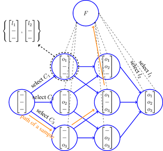
The process of classifying a sample in the proposed method can be summarized as follows: By entering each sample, a classifier is selected and it classifies the sample. Based on the result, another classifier is selected and it also classifies the sample. Now according to the results of the two previous classifiers, the third classifier is selected and it also classifies the sample. At each step, according to the result of the previous classifiers, a new classifier is selected or the process ends and a final label is determined for the sample.
As is clear from the above scenario, these steps can be expressed as a Markov decision process. The output of the classifier is kept in a vector that specifies the state. At the beginning of the sample entry, the output of all classifiers is unknown $([---]) .$ Suppose that the third classifier is selected and outputs its label, the vector of classifiers output becomes as $([--$$\left.o_{3}\right]$. Then the first classifier is selected and the vector of classifiers output becomes $\left(\left[o_{1}-o_{3}\right]\right) .$ Now suppose the final label for the sample is determined and the classification of sample by the ensemble finishes. This process from the start state and performing actions to reach the final state (which is referred to as a period) is depicted in Figure 1 as arrows that specify a path from start to end state.
Figure 1 depicts the implemented MDP symbolically. The results of the classifiers form the state vector. By assigning the final label to the input sample, the system enters the end state. Two types of actions are defined: Select a classifier and select the final label for the input sample. A select label action brings the system to the final state. The reward of each classifier select action is determined by the cost of using that classifier, which includes the test-cost. The reward for the label select actions is also determined by the cost of the misclassification. It should be noted that, as shown in the upper left corner of the Figure 1, in order to abbreviate the shape each circle represents several states, because instead of the output label of each classifier, it is only specified that each classifier has generated its label or not.
Figure 1. Classifying a sample from start state to final state (an episode) in the proposed method
The problem is formulated as a Markov decision process (MDP). A MDP, which is represented by $M,$ is a 4 -tuple $(S, A, T, R)$ in which $S$ is the state space, $A$ is the action space, $T\left(a, s, s^{\prime}\right)$ is the transition function that shows the probability of going to $s^{\prime}$ by performing $a$ in $s,$ and $R(s, a)$ is the reward function that shows expected one-step reward by performing action $a$ in state $s .$ The goal of Reinforcement Learning algorithms is to find the optimal policy $\pi^{*}(s)$ that maps the states to acitons acitons so that the "Discounted Cumulative Reward" is maximized.
In our problem, we have the following definitions:
As stated in the formal definition, the input sample is not directly inserted into the state. if some or all of the features of the input sample be included in the state, the MDP will start from the state corresponding the values of those features. This state definition can be very useful for a faster selection of appropriate classifiers for the sample. But instead, it causes a massive increase in the size of the state space. The space of features itself is so large that in most cases that it cannot be learned by a simple learner. Now, if the result of the outputs of the classifiers is also placed next to it, the state space expands exponentially, which means that it will be overwhelming more than before.
Although the proposed method does not insert the input sample features directly into the state, but it can be seen that the sample indirectly affects the selection of the classifiers. To prove this, we may consider a simple scenario as follows: Assume that using the i-th feature of the input sample in the first steps is very effective in correct classification of it. Also, assume that there is a classifier that only uses this feature. So using this classifier at the beginning of the classification process can have the same effect as entering the i-th feature in the state definition. The claim of the proposed method is that it will use any classifier in its appropriate place, so the intended classifier will be placed in the first steps, and the same effect as using that feature will be created approximately. Therefore, if appropriate and sufficient set of classifiers are used, it can be expected that the advantages of using the features in the state will be relatively achieved.
The proposed method has been evaluated in two synthetic problems, one simple and one complex, to verify the efficiency of the proposed method. In both problems we will change the cost of features and see how the method reacts and adapts itself to minimize the cost.
4.1 Two dimensional lines
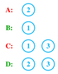
A two-dimensional space is considered, in which each sample has two features of "x" and "y". The problem is binary classification problem, so each sample has a positive or negative label. Each classifier is a line that divides the space into two parts. To test the proposed method, three classifiers (lines) are considered. Two of classifiers use only one feature, and the third one requires both features for classification. The three lines divide the space into seven areas, in four of which train samples exist. Areas are selected so that two areas can be separated from the rest of the space by a single line, but the other two areas at least need two lines to be separated from other areas (Figure 2).
The number of samples in the areas "A" and "B" are the same with each other and twice the number of samples in the areas "C" and "D", the number of samples of the areas "C" and "D" are also equal to each other. The Figure 3 shows the minimum classifiers needed to separate each area.
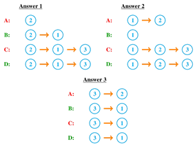
However, since during the classification, the algorithm has no information about the regions and should follow a sequence of classifiers to find the class of the input sample, the optimal answer to the problem using the proposed method is one of the three answers of Figure 4.
Figure 2. The two dimensional problem and samples distribution in areas
Figure 3. Minimum classifiers needed to separate each area in the two dimensional lines problem
Figure 4. Optimal answers to the problem using the proposed method
For clarification consider the "Answer 1". By entering a sample, the method uses "classifier 2". If it classifies the sample into its top side, it is obvious that the sample belongs to area "A" and the method gives a positive output label. Otherwise the "classifier 1" is used. If "classifier 1" classify the sample into its left side, the sample belongs to area "B" and the method gives a negative output label. Otherwise the "classifier 3" is used and its output specifies that the sample is located in which area "C" or "D", so the method gives the corresponding output label.
To prove the effectiveness of the proposed method, two separate scenarios are considered for implementation. In the first scenario, the test-cost is considered zero and in fact the problem is assumed without the test-cost. In the latter scenario, different cost values for each feature are considered to determine whether the proposed method tends to use less costly features.
Table 1. Results of implementation of proposed method for without test-cost scenario
|
Answer Num. |
Probability |
|
1 |
0.48425 |
|
2 |
0.48225 |
|
3 |
0.335 |
Table 2. Results of implementation of proposed method for with test-cost scenario
|
$\cos t(x)=3 \times \cos t(y)$ |
$\cos t(y)=3 \times \cos t(x)$ |
||
|
Answer Num. |
Probability |
Answer Num. |
Probability |
|
1 |
0.003 |
1 |
0.995 |
|
2 |
0.997 |
2 |
0.005 |
|
3 |
0 |
3 |
0 |
In the scenario without test-cost, no feature cost is considered, that is, it is assumed that the use of the features has no cost. Only the use of each classifier has a fixed cost. Since responses 1 and 2 in Figure 4 use the least number of classifiers for the samples, it is expected that they be the most probable answers. The results of this scenario, as shown in the Table 1, confirm this; In the scenario with the test-cost, the use of each of the two features requires cost. This scenario is divided into two sub-scenarios: 1. The cost of the property "x" is three times the cost of the property "y". 2. The cost of the property "y" is three times the cost of the property "x". In the first sub-scenario, where the "x" is more costly, the results are expected to tend to the answer 1 of Figure 4, and in the second sub-scenario, where "y" is more costly, the results are expected to tend to the answer 2 of Figure 4. The results of the implementation shown in the Table 2 confirm this.
4.2 3D Gaussian distributions
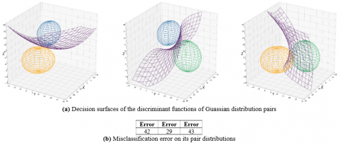
Consider a three class problem in a three-dimensional space. Samples of each class are drawn from a Gaussian distribution $N(\mu, \Sigma)$ with diagonal covariance matrix, i.e., $\forall i, j \in\{1,2,3\}, i \neq j \Rightarrow \sigma_{i, j}=0$. For a better view, the hyperellipsoid of loci of points with a constant density has been drawn for each Gaussian distribution in Figure 5.
Figure 5. The two dimensional problem and samples distribution in areas
As stated in the research [32] the minimum-error-rate classification can be achieved by use of the discriminant functions. The discriminant function of normal distributions $N\left(\mu_{i}, \Sigma_{i}\right)$ is presented in Eq. (3).
$g_{i}(x)=-\frac{1}{2}\left(x-\mu_{i}\right)^{t} \Sigma_{i}^{-1}\left(x-\mu_{i}\right)-\frac{d}{2} \ln 2 \pi-\frac{1}{2} \ln \left|\Sigma_{i}\right|+\ln P\left(\omega_{i}\right)$ (3)
where, In denotes natural logarithm, $d$ denotes number of dimensions and $P\left(\omega_{i}\right)$ denotes prior probability of class $i$ since the covariance matrices are different for each distribution, the only term can be dropped from Eq. (3) is the $\left(\frac{d}{2}\right) \ln 2 \pi .$ So the discriminant functions have the quadratic form of Eq. (4). The decision surfaces of the discriminant functions of each pair of our Gaussian distributions, which has some form of hyperquadrics, are shown in Figure 6.
$g_{i}(x)=x^{t} W_{i} x+w_{i}^{t} x+\omega_{i 0}$ (4)
Figure 6. Three discriminant function classifiers
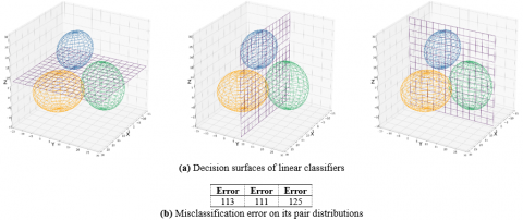
Figure 7. Three linear classifiers which use only one feature for classification
Although above mentioned discriminant functions may yield the minimum error in classification, but also each one uses all the features of the input sample. So using them in our ensemble without adding any other classifier, will force the system to use all features of the sample. To give our ensemble the opportunity to use some less feature consuming classifiers, three simple linear classifiers are added to system. Each of these classifiers is a hyperplane perpendicular to one of the axes, so only uses one attribute of sample to classify it. Figure 7 shows these classifiers.
To evaluate the ability of the proposed method to decrease the test-cost, two ensembles are compared to each other. In the first ensemble all six classifiers, i.e. three Gaussian discriminant functions and three hyperplanes are offered (hereafter called as "6-class ensemble"). So we expect the algorithm to suitably use these classifiers to control the test-cost. But in the second ensemble we only offered three Gaussian discriminant functions to the ensemble (hereafter called as "3-class ensemble"). So the second ensemble is used to see the results without the ability to use less attributes of the input samples. Both ensembles are tested with a range of test-cost, from low to high test-cost to observe the reaction of the proposed method and evaluate its performance in controlling the features cost.
For training of both ensembles, Q-learning with the same parameters is used. The value iteration update formula of $\mathrm{Q}$ learning is shown in Eq. (5). Training is divided into 5000 epoch stages. The Q-learning parameters are set as follows: At the beginning of each stage, the learning rate $(\alpha)$ is set to 0.05 and decays at each epoch to become 0 at the end of stage. At the beginning of the next stage, again the learning rate will be set to 0.05 and so on. An $\varepsilon$ -greedy policy is used in training and the $\varepsilon$ has the same cycle as learning rate, i.e., initialize to 0.2 at the beginning of each stage, and decay to reach 0 at the end of stage. The discount factor $(\gamma)$ is set to 0.9 and is constant all the time. At the end of each stage ( 5000 epoch) the learner is tested and the feature costs are increased, i.e., after each stage the learning is stopped, the learner is tested on a test set, then the feature costs are increased and then the learning is started again and continued with the new costs. Figure 8 shows the diagrams of test-cost and misclassification error in terms of test-cost increase, for both ensembles on the test set.
It is apparent from Figure 8(a) that for the 3-class ensemble, the test-cost increases linearly with increase in features cost. Obviously its use of all features is due to its bad classifiers, all of which use all the features so it has no choice to use less features. But the 6-class ensemble has the opportunity to select those of its classifiers which use less features. Therefore, at the beginning where the features cost is low, the method prefers to use discriminant classifiers because they yield better classification results, but with increase in features cost, the method tends to sacrifice accuracy in exchange of features cost. This shift to use the hyperplane classifiers is first appeared when the features cost is 4. The increase in misclassification error in the corresponding point in Figure 8(b) confirms this shift. The features cost of 7 is another point in which the method decides to increase misclassification error in favor of decrease in features cost.
In fact, there is a trade-off between misclassification error and feature cost which means that to reduce the features cost the method has no choice except to increase the misclassification error. This is an issue imposed by the definition of the current problem and is not a general property of the proposed method. Two set of classifiers are available in this problem, one set has high accuracy but use all features, and another set has less accuracy but use less features. Therefore, the ensemble has no other choice but to select and should accept decrease in accuracy to decrease the feature cost. But suppose that there was plenty of classifiers from which the ensemble was free to use, in such situation the ensemble may find set of classifiers which uses less features, but does not increases the misclassification error. In fact, the proposed method is seen as a classifier selector which aims to find the best arrange of classifiers to minimize the features cost and maximize the accuracy simultaneously.
Figure 8. Results of running the proposed method on 3d gaussian distributions problem
In this paper, a method for test-cost sensitive classification is proposed. The basis of the proposed method is to organize classifiers using reinforcement learning so that the best arrange of classifiers with the aim of minimizing test-cost is found for each sample. Although the idea behind this method is not so complex, but it is very useful and helpful to deal with the hard problem of run-time cost. The results of the proposed method on the two problems show that the proposed method behaves as expected and finds the least cost arrange of classifiers as feature cost increases.
The contribution of the proposed method in the Test-Cost sensitive classification domain is summarized as follows: 1. Instead of looking at the features themselves, it uses the classifiers and allows the selection of them to determine the features to use. This is more practical than selecting the features first, because after that the right classifier should be found that can do the classification well with the selected features. 2. Problem formulation as MDP, so that the features themselves are not included in state, which results a massive decrease in state space. Instead the method relies on the result of the used classifiers to find the next suitable classifiers to use.
The ability of the proposed method to find the best set between classifiers, reaches it maximum performance when a large number of classifiers is provided for it. Therefore, the method can choose suitable classifiers and even increase the number of classifiers needed to classify samples with the aim of using less features. But this increase in number of classifiers has another effect, the known problem of high-dimensional state space in RL methods. Popular solutions such as using Neural Networks may be used to solve this problem, but a hopeful future work is to find problem-specific solutions to address it.
[1] Contardo, G. (2017). Machine learning under budget constraints. Doctoral dissertation. Université Pierre et Marie Curie-Paris VI.
[2] Weiss, G., Saar-Tsechansky, M., Zadrozny, B. (2005). Report on UBDM-05: Workshop on utility-based data mining. ACM SIGKDD Explorations Newsletter, 7(2): 145-147. https://doi.org/10.1145/1117454.1117477
[3] Weiss, G.M., Tian, Y. (2007). Maximizing classifier utility when there are data acquisition and modeling costs. Data Mining and Knowledge Discovery, 17(2): 253-282. https://doi.org/10.1007/s10618-007-0082-x
[4] Bolukbasi, T. (2018). Machine learning in the real world with multiple objectives. Doctoral dissertation. Boston University.
[5] Alpaydin, E. (2009). Introduction to Machine Learning. MIT Press.
[6] Viola, P., Jones, M.J. (2004). Robust real-time face detection. International Journal of Computer Vision, 57(2): 137-154. https://doi.org/10.1023/b:visi.0000013087.49260.fb
[7] Bourdev, L., Brandt, J. (2005). Robust object detection via soft cascade. 2005 IEEE Computer Society Conference on Computer Vision and Pattern Recognition (CVPR'05), San Diego, CA, USA, pp. 236-243. https://doi.org/10.1109/cvpr.2005.310
[8] Chen, M., Xu, Z., Weinberger, K., Chapelle, O., Kedem, D. (2012). Classifier cascade for minimizing feature evaluation cost. Artificial Intelligence and Statistics, 218-226.
[9] Xu, Z., Weinberger, K.Q., Chapelle, O. (2012). The greedy miser: Learning under test-time budgets. Proceedings of the 29th International Conference on Machine Learning, pp. 1299-1306.
[10] Grubb, A., Bagnell, D. (2012). Speedboost: Anytime prediction with uniform near-optimality. Artificial Intelligence and Statistics, 458-466.
[11] Andrade, D., Okajima, Y. (2019). Efficient Bayes risk estimation for cost-sensitive classification. The 22nd International Conference on Artificial Intelligence and Statistics, pp. 3372-3381.
[12] Gao, T., Koller, D. (2011). Active classification based on value of classifier. Advances in Neural Information Processing Systems, 1062-1070.
[13] Ji, S., Carin, L. (2007). Cost-sensitive feature acquisition and classification. Pattern Recognition, 40(5): 1474-1485. https://doi.org/10.1016/j.patcog.2006.11.008
[14] Dulac-Arnold, G., Denoyer, L., Preux, P., Gallinari, P. (2012). Sequential approaches for learning datum-wise sparse representations. Machine Learning, 89(1-2): 87-122. https://doi.org/10.1007/s10994-012-5306-7
[15] Dulac-Arnold, G., Denoyer, L., Thome, N., Cord, M., Gallinari, P. (2014). Sequentially generated instance-dependent image representations for classification. The International Conference on Learning Representations (ICLR 2014).
[16] Janisch, J., Pevný, T., Lisý, V. (2019). Classification with Costly Features Using Deep Reinforcement Learning. Proceedings of the AAAI Conference on Artificial Intelligence, 33: 3959-3966. https://doi.org/10.1609/aaai.v33i01.33013959
[17] Janisch, J., Pevný, T., Lisý, V. (2020). Classification with costly features as a sequential decision-making problem. Machine Learning, 1-29. https://doi.org/10.1007/s10994-020-05874-8
[18] He, H., Daumé III, H., Eisner, J. (2012). Cost-sensitive dynamic feature selection. The International Conference on Machine Learning (ICML) workshop on Inferning: Interactions between Inference and Learning, Edinburgh, Scotland, UK.
[19] Shim, H., Hwang, S.J., Yang, E. (2018). Joint active feature acquisition and classification with variable-size set encoding. Advances in Neural Information Processing Systems, pp. 1368-1378.
[20] Peng, Y.S., Tang, K.F., Lin, H.T., Chang, E. (2018). Refuel: Exploring sparse features in deep reinforcement learning for fast disease diagnosis. In Advances in Neural Information Processing Systems, pp. 7322-7331.
[21] Trapeznikov, K., Saligrama, V., Castañón, D. (2013). Multi-stage classifier design. Machine Learning, 92(2-3): 479-502. https://doi.org/10.1007/s10994-013-5349-4
[22] Contardo, G., Denoyer, L., Artières, T. (2016). Recurrent neural networks for adaptive feature acquisition. Lecture Notes in Computer Science, 591-599. https://doi.org/10.1007/978-3-319-46675-0_65
[23] Kachuee, M., Darabi, S., Moatamed, B., Sarrafzadeh, M. (2019). Dynamic feature acquisition using denoising autoencoders. IEEE Transactions on Neural Networks and Learning Systems, 30(8): 2252-2262. https://doi.org/10.1109/tnnls.2018.2880403
[24] Zhan, Y., Da, Q., Xiao, F., Zeng, A.X., Yu, Y. (2018). Accelerating E-commerce search engine ranking by contextual factor selection. arXiv preprint arXiv:1803.00693.
[25] Benbouzid, D., Busa-Fekete, R., Kégl, B. (2012). Fast classification using sparse decision DAGs. In Proceedings of the 29th International Conference on Machine Learning, pp. 747-754.
[26] Karayev, S., Baumgartner, T., Fritz, M., Darrell, T. (2012). Timely object recognition. Advances in Neural Information Processing Systems, pp. 890-898.
[27] Deng, J., Satheesh, S., Berg, A.C., Li, F. (2011). Fast and balanced: Efficient label tree learning for large scale object recognition. Advances in Neural Information Processing Systems, pp. 567-575.
[28] Xu, Z., Kusner, M., Weinberger, K., Chen, M. (2013). Cost-sensitive tree of classifiers. International Conference on Machine Learning, pp. 133-141.
[29] Weiss, D., Sapp, B., Taskar, B. (2013). Dynamic structured model selection. 2013 IEEE International Conference on Computer Vision, Sydney, NSW, pp. 2656-2663. https://doi.org/10.1109/iccv.2013.330
[30] Chen, Y., Shioi, H., Montesinos, C.F., Koh, L.P., Wich, S., Krause, A. (2014). Active detection via adaptive submodularity. In International Conference on Machine Learning, 32(1): 55-63.
[31] Maliah, S., Shani, G. (2018). MDP-based cost sensitive classification using decision trees. In Thirty-Second AAAI Conference on Artificial Intelligence.
[32] Duda, R.O., Hart, P.E., Stork, D.G. (2012). Pattern Classification. John Wiley & Sons.