Yakoub Boukhari
© 2020 IIETA. This article is published by IIETA and is licensed under the CC BY 4.0 license (http://creativecommons.org/licenses/by/4.0/).
OPEN ACCESS
The weight loss of raw materials during cement clinker production is often used as an indicator of final product quality. The raw materials are usually limestone mixed with a sand, clay and iron ore. The weight loss is influenced by essentials parameters such as the correct composition, particle size, temperature and duration of burning of the raw materials. It is difficult to determine experimentally the weight loss with high accuracy due to the interaction of its several parameters. Moreover, the determination of the weight loss is expensive, time-consuming, risk associated. Consequently, various intelligent models such as artificial neural network optimized by genetic algorithm (GA-ANN), regression tree ensembles (RTE), least squares support vector machines (LS-SVM), adaptive neuro-fuzzy inference system (ANFIS) are proposed in the present paper to predict the weight loss. The performance of these models is also compared. The results show that all models have great ability as feasible tools and as good alternatives to predict the weight loss quickly, efficiently and less expensive compared to experiment measurements. According to the values of adjusted R2 there are 99.31%, 99.06%, 98.01% and 97.17% of data can explained by GA-ANN, RTE, LS-SVM, ANFIS respectively with error less than 3.1%.
adaptive neuro-fuzzy inference system, artificial neural network, clinker, genetic algorithm, least squares support vector machines, regression tree ensembles, weight loss
Cement is the most widely consumed construction material on the planet. The global cement production across the world grew from 3.3 billion tonnes in 2009 [1] to 3.6 billion tonnes in 2012 [2]. The cement is produced by adding small quantity of gypsum to cement clinker. The clinker is made by burning a homogeneous mixture of raw material at high temperature in a rotary kiln and then cooled by fresh air. The clinker production process [3] used up to 70% or more of the total fuel [4]. The quality of clinker is principally controlled by appropriate selection of raw materials. The main raw material for clinker production is usually limestone mixed with a sand, clay and iron ore in definite mass percentages [5].
The weight loss of raw materials during cement clinker production is often used as an indicator of final product quality. In fact, many factors such as the chemical composition, particle size distributions, temperature range and burning time have great influence on the precise experimental determination of the weight loss. The weight loss is very complex, nonlinear phenomena and hard to quantise mathematically or even impossible with accuracy due to the interaction of its parameters [6]. Moreover, the determination of the weight loss is expensive, time-consuming, require chemical treatments, risks associated and care when taking test samples. Therefore, it is required and important to research an appropriate model to estimate the weight loss without experimental operation. In fact, the predicting weight loss based on its influenced factors data become challenging.
In recent years, artificial intelligence (AI) is rapidly becoming one of the most important in predicting of complex phenomena. In contrary, it is difficult or even impossible to predict outcome with conventional statistical models [7]. The major advantages of using artificial intelligence is that it does not need the explicit knowledge behavior of phenomena and any kind of mathematical equation in advance [8]. The intelligent models need only to be trained by sufficient data under optimal parameters [9] to predict the target with high performance [10].
In the present study, various artificial intelligence models such as least squares support vector machines (LS-SVM), artificial neural network optimized by genetic algorithm (GA-ANN), regression tree ensembles (RTE) and adaptive neuro-fuzzy inference system (ANFIS) are used to predict the weight loss of raw materials during cement clinker production. These models have shown successful results in the domains of prediction. The ensemble boosted trees has achieved a good prediction performance on the bankruptcy prediction [11] and for the prediction of airfoil self-noise [12]. GA-ANN can be used quite satisfactorily to predict flatness value of hot rolled strips [13] and natural fractures in low permeability reservoirs [14]. ANFIS shows satisfactory performance in the prediction of half-cone geometry in dam reservoirs [15] and CO2 capture process [16]. LS-SVM can estimate with performance the Escherichia coli promoter gene sequences [17] and of barite deposition [18]. The remainder of this paper is organized as follows. Section 2 aims to provide a brief overview of models theory. Section 3 describes the experimental methods and materials used to determine the weight loss of raw materials. The results obtained are given, discussed and compared to experimental results in section 4. Finally, section 5 presents our conclusions.
2.1 Adaptive neuro-fuzzy inference system (ANFIS)
Adaptive neuro-fuzzy inference system (ANFIS) developed by Jang (1993) [19] is a very powerful approach for modelling complex and nonlinear relationship between input and output data than conventional statistical methods. It is combination of artificial neural network and fuzzy logic (LF) to exploit the advantages of both, learning capabilities of ANN and reasoning of fuzzy logic through the use of fuzzy rules IF–THEN. The advantageous of ANFIS include easy implementation, good learning ability, short time of learning, soft and hard decisions [20] and strong generalization abilities [21]. The learning rule of ANFIS uses the hybrid method, the back-propagation used in the common feed-forward neural networks and the least square for the parameters associated with the input and output membership functions respectively [22]. There are two types of fuzzy inference system FISs described in the literature Mamdani and Sugeno FIS. Sugeno type fuzzy inference system with two fuzzy if-then rules is the most widely applied to generate and to facilitate learning and adaptation [23]. Several parameters of ANFIS such as type and number of membership function, maximum number of training epochs and type of fuzzy inference system are carefully chosen to achieve satisfying results. The parameters of ANFIS are set and adjusted during the training process.
2.2 Least square support vector machine (LS-SVM)
LSSVM proposed by Suykens and Vandewalle [24] is also one of the most powerful tools to solve nonlinear problem [25]. The main advantage of LSSVMs over SVMs is solving a set of linear equations instead of a quadratic programming. LS-SVM uses square errors instead of nonnegative errors in the cost function to reduce computing complexity. Many Kernel functions are used and implemented in LS-SVM learning methods; linear, polynomial (Poly), radial basis function (RBF), or sigmoid-shaped function [26]. Gaussian radial basis kernel (RBF) is the most popular and commonly used to approximate the nonlinear systems [27]. The predictive of LS-SVM is directly influence by its two main hyper-parameters while the other techniques require more adjustable parameters. Two principal hyper-parameters of LS-SVM are namely regularization parameter, gamma (γ) and squared bandwidth, sigma (σ2). These parameters are selected carefully to avoid overfitting and underfitting problem. Full names of authors are required. The middle name can be abbreviated.
2.3 Genetic algorithm artificial neural network (GA-ANN)
The hybrid GA–ANN is a combination of the artificial neural network (ANN) and Genetic algorithm (GA). It is one of the most important and powerful prediction techniques [28]. Usually, the overfitting and the local minima in the neural network learning process are inevitable in the searching for optimal weights [29]. To obtain the global optimal solution and without being trapped in local minima, GA algorithm is used to train and to optimize the initial parameters value of ANN [30]. This advantage is essentially related on the good choice of its essential parameters.
The basic idea of GA is to imitate the concepts of natural selection and genetics. It is an appropriate optimization technique [31] for all kinds of nonlinear optimization systems. The main parameters of GA are population size and generation number. In general, the initial population (individuals) is randomly chosen and then evaluated to create a new better population for the next generation. The new better population are updated and are evaluated at each generation. Three genetic operators, such as selection, crossover and mutation are applied by GA to generate new generation [32]. This procedure is repeated until the termination criterion is satisfied. The artificial neural networks (ANN) are inspired by a biological neural system to emulate brain functions with capability to learn and then to predict based on from training data [33]. The ANN is composed of successive layers: input layer, one or more hidden layers and output layer [34]. These layers are formed by one or more neurons which are connected by to every node in the next layer by the connection weight and biases. The Levenberg–Marquardt (LM) back propagation (BP) algorithm of ANN is used to iteratively adjust weight and biases [35] until the convergence mean square error between experimental and predicted values is achieved. In general, the purpose of the training process is found the optimum architecture of ANN, number of hidden layer, number of neurons in the hidden layer, transfer functions of both hidden and output layers. These parameters are chosen after a series of trials during training process.
2.4 Regression Tree Ensembles (RTE)
Regression trees are widely used in prediction fields. The instability of regression trees due to perturbations in the training introduces uncertainty in their prediction ability and their interpretation [36]. For increasing predictive performance, multiple regression trees are combined to form regression tree ensemble. The most popular ensembles models of regression trees are bagging, boosting and random forest that are used to increase the performance of unstable learners [37]. Boosting algorithm [38] method used in this paper is powerful learning techniques. It is a stage-wise process that aggregates information from several trees to minimize the loss function by iteratively applying. A series of weak learners (regression trees) are combined to achieve a final powerful learner. The parameters used to build RTE model are maximal number of decision splits, minimum number of branch node observations, minimum number of leaf node observations, ensemble-aggregation method, number of ensemble learning cycles and quadratic error tolerance per node.
3.1 Materials and experiments
The experimental study used the main following raw materials, limestone, sand, clay and iron ore. Four groups are prepared with different combination of each compound. The raw materials mixture composition (% by weight) of each group are summarised in Table 1. The compounds of each group are grinded and then classified into following particle size distribution: 71µm, 125µm, 250µm and 350µm.
The experimental study is divided into two parts. First part, each group with different particle size distribution (71, 125, 250 and 350µm) is burned at a temperature of 1000°C for various periods of time (5, 10, 15, 20 and 30 min) in a muffle furnace of laboratory as shown in Table 2. Second part, only the first and the last groups with particles size of 350 µm are burned at several constant temperatures (600, 700, 800, 900 and 1000°C) for 20 min as shown in Table 3. The number of experiments collected during the first part and second parts are 80 and 10 experiments respectively.
Table 1. Raw materials mixture composition (% by weight) of each group
|
Group |
limestone |
Sand |
Clay |
Iron ore |
|
Group 1 |
100 |
- |
- |
- |
|
Group 2 |
85 |
15 |
- |
- |
|
Group 3 |
83 |
15 |
2 |
- |
|
Group 4 |
82.5 |
14.5 |
2 |
1 |
Table 2. Each group with different particle size is burned at a temperature of 1000°C for various periods of time
|
Particle size (µm) |
Time (min) |
||||
|
5 |
10 |
15 |
20 |
30 |
|
|
71 |
+ |
+ |
+ |
+ |
+ |
|
125 |
+ |
+ |
+ |
+ |
+ |
|
250 |
+ |
+ |
+ |
+ |
+ |
|
310 |
+ |
+ |
+ |
+ |
+ |
Table 3. First and the last groups with particles size of 350 µm are burned at several constant temperatures for 20 min
|
Group |
Temperature (°C) |
||||
|
600 |
700 |
800 |
900 |
1000 |
|
|
Group 1 |
+ |
+ |
+ |
+ |
+ |
|
Group 4 |
+ |
+ |
+ |
+ |
+ |
The weight loss is determined for each sample by weighing it before (Wi) and after (Wf) burning. It is calculated by dividing the difference of weight by the initial weight, then multiplying the result by 100 to represent it as a percentage as Eq. (1).
$W L(\%)=\frac{W_{i}-W_{f}}{W_{i}} * 100$ (1)
3.2 Data acquisition
The result obtained are collected in a total data table (90 rows x 10 columns) which covers all experimental works. Each experiment is presented by row. The first nine columns are particle size, duration of burning of each sample and temperature. These nine columns are taken as inputs. The last column namely mass loss is taken as output. The total data set is randomly divided into two phases training and testing. The training phase is utilised to build the model. Once model is adequately trained. It is used to predict remaining (testing phase) of data and to evaluate the generalization capability. In order to suitably compare the performance of models, the same percentage of training and testing data are chosen. Several percentages of training and testing data are used in the literature [39, 40]. In this paper, the ratio of 2/3 of the data is used to train the model and remaining data (1/3) are used to judge the generalization capability.
3.3 Model evaluation methods
The performance criteria are statistically measured between experimental and predicted values. Some statistical methods are used to evaluate the performance, such as statistical error analysis and graphical error analysis. The statistical error analysis is usually root mean squared error (RMSE), the coefficient of determination R2, the adjusted R2 (adj), and the mean absolute percent error (MAPE), the scatter index (SI) [41]. The prediction is perfect if the values of R2 and the adjusted R2 are very close to 1. The model is able to predict with a high performance when values of RMSE and MAPE are found very close to zero. The performance is excellent when SI is less than 0.1; good if SI between 0.1 and 0.2; and poor if SI more than 0.3. The most popular graphical error analysis are cross plot and error distribution.
Models used in this study can theoretically approximate any nonlinear by carefully adjusted its parameters. To choose optimal parameters for each model, many experiments are carried out randomly in advance to improve the generalization abilities. The performance of each models is judged only based on testing phase, because it is easy to achieve a high performance based on training process without any increasing the generalisation abilities. All models are implemented in Matlab 2018a.
4.1 ANFIS result
Choosing of optimum parameters during training phases is very important to get good performance. The optimum parameter and their values used to construct ANFIS are illustrated in Table 4.
Table 4. Details of ANFIS model
|
Parameter types of ANFIS |
Value |
|
Membership function |
FCM Clustering |
|
Fuzzy System Type |
Sugeno |
|
Number of rules |
3 |
|
Epoch Number |
120 |
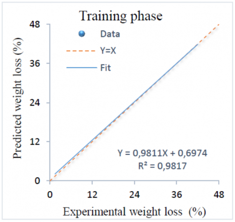
Figure 1. Experimental weight loss versus ANFIS results for training phase
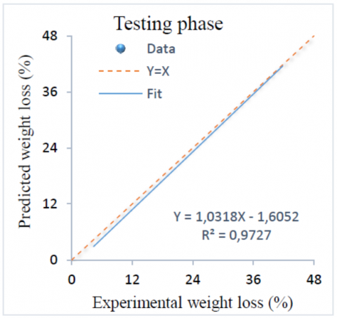
Regression plots of experimentally measured weight loss values and those predicted by ANFIS for training and testing phases are shown in Figure 1 and Figure 2. These figures illustrate that experimental and predicted weight loss are well correlated for both phases. It is clear that representative points are very close to the line of equality. The coefficient of determination R2 are equal to 0.9817 and 0.9727 for the training and testing set respectively. The good performance of ANFIS is also confirmed in these figures.
Figure 2. Experimental weight loss versus ANFIS results for testing phase
Figure 3. Relative error of ANFIS for training phase
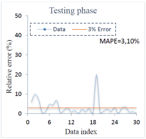
Figure 4. Relative error of ANFIS for testing phase
Distribution of the relative errors between experimental and ANFIS predicted weight loss for training phase and testing phases are shown in Figure 3 and Figure 4. In this case, the majority of the data collapsed between 0% and 2% for training data and between 0% and 3% for testing data. The MAPE of training and testing data obtained are 2.73% and 3.10% respectively.
It is clearly illustrated in Table 5 that ANFIS is able to successfully predict up to 98% of training data and 97% of testing data SI less than 0.1 as shown in Table 5. The results clearly demonstrate that the hybrid model which exploit the advantages learning capability of ANN and reasoning of fuzzy logic, could be successfully used in predicting of weight loss with high degree of performance.
Table 5. Performance criteria for training and testing phases of ANFIS
|
|
R² |
R² adj |
MAPE |
RMSE |
SI |
|
Train |
0,9817 |
0,9814 |
2,73% |
1,1831 |
0,0321 |
|
Test |
0,9727 |
0,9717 |
3,10% |
1,2825 |
0,0346 |
4.2 LS-SVM result
The optimum hyper-parameters of LS-SVM illustrated in Table 6 are selected during the learning process.
Table 6. Details of LS-SVM model
|
Parameter types of LS-SVM |
Value |
|
Kernel function |
RBF |
|
Regularization parameter (γ) |
4550 |
|
Squared bandwidth (σ2) |
8115 |
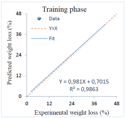
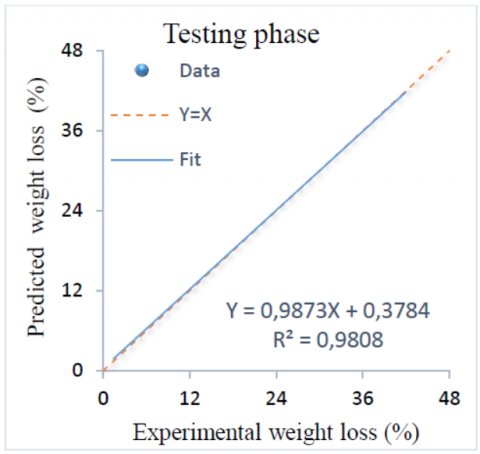
The experimental values of weight loss versus LS-SVM model results for training and testing phases are shown in Figure 5 and Figure 6, respectively. It is found that the R2 for the training and the testing sets are 0.9863 and 0.9808 respectively. Also, it can be seen that the predicted weight loss values are quite close to the experimental values. The equality line of (Y=X) and fit line are superimposed.
Figure 5. Experimental weight loss versus LS-SVM results for training phase
Figure 6. Experimental weight loss versus LS-SVM results for testing phase
Figure 7. Relative error of LS-SVM for training phase
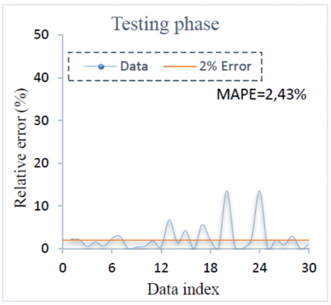
Figure 8. Relative error of LS-SVM for testing phase
Relative errors between the LS-SVM predications and corresponding experimental values of weight loss for both phases are shown in Figure 7 and Figure 8. These figures clearly illustrate the high efficiency of the predictive model. It is also important to observe that more than 57% of testing data have a relative error less 2% and 70% of training data have a relative error less 1%. The MAPE recorded by LSSVM for training and testing phases are 1.41% and 2.43%. The R2 and MAPE obtained validate that LSSVM model is capable to predict the weight loss with high performance.
The performance criteria for training and testing phases of LS-SVM model are presented in Table 7. Based on R² adj and SI value, there are at least 98% of dataset can explain by LS-SVM model with excellent performance and robustness. This is mainly due its appropriate capability for minimizing complexity by SVM, introducing linear equations and using RBF Kernel function.
Table 7. Performance criteria for training and testing phaes of LS-SVM
|
|
R² |
R² adj |
MAPE |
RMSE |
SI |
|
Train |
0,9863 |
0,9861 |
1,41% |
0,9656 |
0,0262 |
|
Test |
0,9808 |
0,9801 |
2,43% |
1,1153 |
0,0303 |
4.3 RTE result
The generalization learning capability of RTE highly dependent upon on the selection of its learning parameters. The optimum parameters of regression tree ensembles utilised to achieve maximum accuracy are summarized in Table 8.
Table 8. Details of RTE model
|
Parameter types of RTE |
Value |
|
Maximal number of decision splits |
2 |
|
Minimum number of branch node observations |
12 |
|
Minimum number of leaf node observations |
2 |
|
Ensemble-aggregation method |
LSBoost |
|
Number of ensemble learning cycles |
200 |
|
Quadratic error tolerance per node |
10-3 |
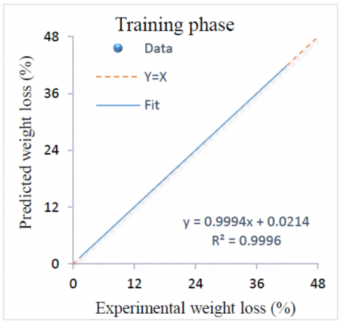
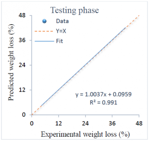
The experimental values of weight loss versus RTE model results for training and testing data are shown in Figure 9 and Figure 10 respectively. As shown in these figures, predicted weight loss for two phases using RTE are in appropriate agreement with experimental results. It is clear that data dispersion mostly lies around the line (Y=X), implying a very excellent closeness between the excremental and predictive data. The fit of data is expressed by R2, which are found to be 0.9996 and 0.9910 for training and testing respectively.
Figure 9. Experimental weight loss versus RTE results for training phase
Figure 10. Experimental weight loss versus RTE results for testing phase
Figure 11. Relative error of RTE for training phase
Figure 12. Relative error of RTE for testing phase
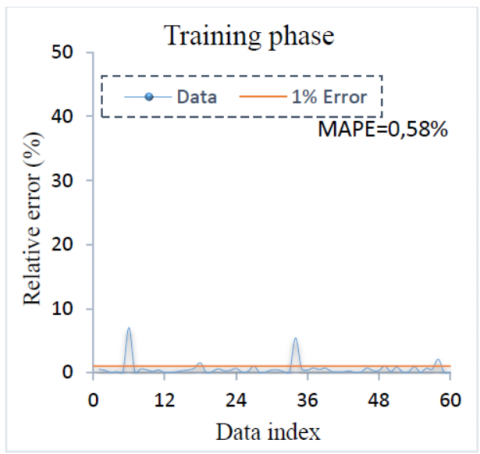
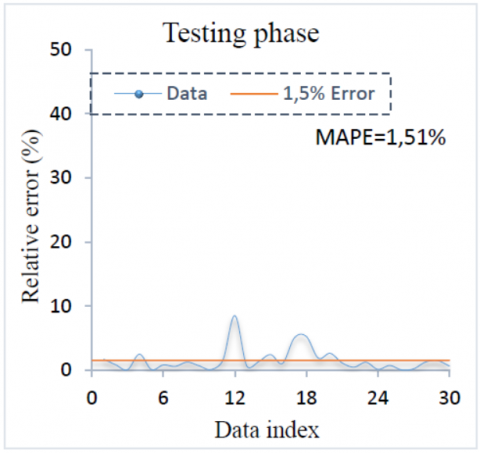
The relative error distributions for training and testing data are shown in Figure 11 and Figure 12. The results predicted by RTE are almost obtained with error less than 1.5% for testing data and less than 1% for training data and even approximating zero, indicating really very small deviations between the predicted and experimental values. These figures exhibit the excellent performance of the RTE prediction. Thus, the high learning and generalisation ability of the RTA can be emphasised. The MAPE value are 0.58% for training and 1.51% for testing data. Besides, practically difference between experimental and predicted values remain at the interval of [0, 1.5%].
The performance criteria for the training and the testing data are presented in Table 9. The adjusted R2 value are 0.9996 for training data and 0.9906 indicate that only 0.04% of training and 0.90% of testing data are not explained by this model. The SI value less than 0.1 for both phases are indicative of the excellent accuracy. The best performance obtained by RTE reflect the powerful of boosting with a large tree size and optimum parameters used. Finally, the results justify that RTE is effectively used for predicting weight loss as a powerful technique.
Table 9. Performance criteria for training and testing phases of RTE
|
|
R² |
R² adj |
MAPE |
RMSE |
SI |
|
Train |
0,9996 |
0,9996 |
0,58% |
0,1722 |
0,0048 |
|
Test |
0,9910 |
0,9906 |
1,51% |
0,6704 |
0,0175 |
4.4 GA-ANN result
Many experiments carried out randomly to choose optimum parameters which are shown in Table 10.
Table 10. Details of GA-ANN model
|
Parameter types of RTE |
Value |
|
Number of hidden layers |
2 |
|
Number of neurons in the hidden layer |
12 |
|
Activation functions in hidden layers |
tansig |
|
Activation functions in output layer |
purelin |
|
Population size |
10 |
|
Number of Generation |
15 |
Figure 13. Experimental weight loss versus GA-ANN results for training phase
The experimental values of weight loss versus GA-ANN results for training and testing dataset are shown in Figure 13 and Figure 14. These figures show the regression analysis of the ANFIS. The coefficient of determination R2 values for training and testing data are 0.9969 and 0.9933 respectively. The values of R2 indicate an excellent agreement between the experimental and model prediction values and confirm the excellent predictive ability of GA-ANN model.
Figure 14. Experimental weight loss versus GA-ANN results for testing phase
Figure 15. Relative error of GA-ANN for training phase
Figure 16. Relative error of GA-ANN for testing phase
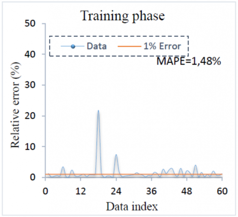
The relative error between experimental and GA-ANN predicted weight loss for training and testing phases are shown in Figure 15 and Figure 16. In general, the relative error distribution of the GA-ANN is very close to the zero line for both phases. It can be noted that the relative error of 60% of training data and 53% of testing data are less than 1%. The obtained MAPE for training and testing data are about 1.48% and 1.42% respectively. It is clear that the very low predictions errors are obtained by GA-ANN.
Performance criteria for training and testing phases of GA-ANN are summarized in Table 11. The value of adjusted R2 means 99.69% of training and 99.33% of testing data are explained by GA-ANN model. It is also observed that the value of adjusted R2 and R2 are very close to 1 while the MAPE, RMSE and SI are close 0. The results show that GA-ANN has an excellent prediction capability. Upper predictive accuracy of hybrid GA-ANN can be attributed to its optimization by GA algorithms and strong learning ability of the ANN.
Table 11. Performance criteria for training and testing phaes of GA-ANN
|
|
R² |
R² adj |
MAPE |
RMSE |
SI |
|
Train |
0,9969 |
0,9969 |
1,48% |
0,4757 |
0,0127 |
|
Test |
0,9933 |
0,9931 |
1,42% |
0,4757 |
0,0127 |
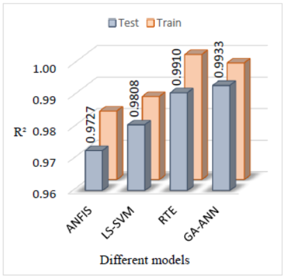
4.5 Comparison between the intelligent models
A comparative study is conducted in terms of MAPE and R2, to compare the generalization capability of models is shown in Figure 17 and Figure 18. These figures provide a comparative summary of the R2 and MAPE for different methods. It is clear that the smallest error and highest R2 are obtained by GA-ANN while the highest error and smallest R2 are obtained by ANFIS. The prediction capability of ANN optimized by GA as powerful optimisation technique is better than that of ANN used reasoning of fuzzy logic. It is evident that GA-ANN model has a little higher accuracy compared to the RTE model, it is better because it uses powerful optimization technique (GA) and powerful of boosting algorithms. Moreover, the results obtained revealed that the LS-SVM and ANFIS are also capable to predict weight loss with high accuracy. Moreover, there is no significant difference between LS-SVMN and ANFIS. Results obtained LS-SVM are expected because it can to reduce the effect of noise in conventional regression model and tackle the nonlinear of weight loss phenomena and maximize the margin.
Figure 17. Comparison between models in term of R2
Figure 18. Comparison between models in term of MAPE
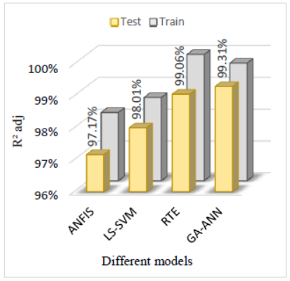
Figure 19. Comparison between models in term of R2 adj
Figure 20. Comparison between models in term of SI
In addition, results predicted by all models are also compared in the terms of adjusted R2 and SI. The adjusted R2 and SI obtained between experimental and predicted by all models are shown in Figure 19 and Figure 20, respectively. Based on the values of adjusted R2, there are only 0.69%, 0.94%, 1.99% and 2.83% of data are not explained by GA-ANN, RT, LS-SVM and ANFIS respectively. All values of SI obtained are less than 0.1 which mean that all models can predict weight loss with excellent performance. Lastly, all models proposed are promising techniques for predicting weight loss with high accuracy and without any sign of overfitting or underfitting. On the other words, all models are considered good alternatives to determine the weight loss.
The relation between the weight loss of raw materials during cement clinker production and its influence factors namely, the composition, size particles, temperature and duration of burning is highly nonlinear and more complicated. In the present paper, GA-ANN, LS-SVM, RTE and ANFIS models are developed for predicting the weight loss.
The results obtained by applying all models under the optimum condition show a high degree of correlation between experimental and predict weigh loss with low errors, indicating that the prediction can be carried out very accurately in this way. The lowest error and highest R2 values are obtained by GA-ANN, whereas the highest error and lowest R2 values are obtained by ANFIS.
The values of adjusted R2 mean that only 0.69%, 0.94%, 1.99% and 2.83% of data are not explained by GA-ANN, RT, LS-SVM and ANFIS respectively. The values of MAPE of GA-ANN, RTE, LS-SVM and ANFIS are about 1.41%, 1.51%, 2.43% and 3.10 % respectively. Moreover, the values of SI (<0.1) obtained are indicative of the excellent accuracy. Finally, all models proposed are mainly attractive and promising techniques for predicting weight loss with high accuracy and without any sign of overfitting or underfitting. On the other words, models are considered good alternatives to determine the weight loss quickly, efficiently and less expensive compared to experiment measurements, whenever the experiment is costly, risks associated and time consuming, uncomfortable. According to the values of R2, adjusted R2, MAPE and RMSE obtained by each model in the testing phase, the prediction efficiency of models increases in the order: GA-ANN>RTE>LS-SVM>ANFIS.
[1] Feiz, R., Ammenberg, J., Baas, L., Eklund, M., Helgstand, A., Marshall, R. (2018). Improving the CO2 performance of cement, part 1: Utilizing life-cycle assessment and key performance indicators to assess development within the cement industry. Journal of Cleaner Production, 98: 282-291. https://doi.org/10.1016/j.jclepro.2014.01.103
[2] Rashad, A.M. (2015). Potential use of phosphor gypsum in alkali-activated fly ash under the effects of elevated temperatures and thermal shock cycles. Journal of Cleaner Production, 87: 717-725. https://doi.org/10.1016/j.jclepro.2014.09.080
[3] Zhang, D., Cai, X., Jaworska, B. (2020). Effect of pre-carbonation hydration on long-term hydration of carbonation-cured cement-based materials. Construction and Building Materials, 231: 117-122. https://doi.org/10.1016/j.conbuildmat.2019.117122
[4] Copertaro, E., Chiariotti, P., Donoso, A.A.E., Peters, N.B., Revel, G.M. (2015). A discrete-continuous approach to describe CaCO3 decarbonation in non-steady thermal conditions. Powder Technology, 275: 131-138. https://doi.org/10.1016/j.powtec.2015.01.072
[5] Young, G., Yang, M. (2019). Preparation and characterization of Portland cement clinker from iron ore tailings. Construction and Building Materials, 197: 152-156. https://doi.org/10.1016/j.conbuildmat.2018.11.236
[6] Lippiatt, N., Ling, T.C., Eggermont, S. (2019). Combining hydration and carbonation of cement using super-saturated aqueous CO2 solution. Construction and Building Materials, 229: 116-825. https://doi.org/10.1016/j.conbuildmat.2019.116825
[7] Boukhari, Y., Boucherit, M.N., Zaabat, M., Amzert, S., Brahimi, K. (2017). Artificial intelligence to predict inhibition performance of pitting corrosion. Journal of Fundamental and Applied Sciences, 9(1): 308-322. http://dx.doi.org/10.4314/jfas.v9i1.19
[8] Boucherit, M.N., Amzert, S.A., Arbaoui, F., Boukhari, Y., Brahimi, A. Younsi, A. (2019). Modelling input data interactions for the optimization of artificial neural networks used in the prediction of pitting corrosion. Anti-Corrosion Methods and Materials, 66(4): 369-378. https://doi.org/10.1108/ACMM-07-2018-1976.
[9] Boukhari, Y., Boucherit, M.N., Zaabat, M., Amzert, S., Brahimi, K. (2018). Optimization of learning algorithms in the prediction of pitting corrosion. Journal of Engineering Science and Technology, 13(5): 1153-1164.
[10] Boucherit, M.N., Amzert, S.A., Arbaoui, F., Hanini, S., Hammache, A. (2008). Pitting corrosion in presence of inhibitors and oxidants. Anti-Corrosion Methods and Materials, 55(3): 115-122. https://doi.org/10.1108/00035590810870419
[11] Zieba, M., Tomczak, S.K., Tomczak, J.M. (2016). Ensemble boosted trees with synthetic features generation in application to bankruptcy prediction. Expert Systems with Applications, 58: 93-101. https://doi.org/10.1016/j.eswa.2016.04.001
[12] Patri, A., Patnaik, K. (2015). Random forest and stochastic gradient tree boosting based approach for the prediction of airfoil self-noise. Procedia Computer Science, 46: 109-121. https://doi.org/10.1016/j.procs.2015.02.001
[13] John, S., Sikdar, S., Swamy, P.K. (2008). Hybrid neural–GA model to predict and minimise flatness value of hot rolled strips. Journal of Materials Processing Technology, 195(1-3): 314-320. https://doi.org/10.1016/j.jmatprotec.2007.05.014
[14] Xue, Y., Cheng, L., Mou, J., Zhao, W. (2014). A new fracture prediction method by combining genetic algorithm with neural network in low-permeability reservoirs. Journal of Petroleum Science and Engineering, 121: 159-166. https://doi.org/10.1016/j.petrol.2014.06.033
[15] Emamgholizadeha, S., Batenib, S.M., Jeng, D.S. (2013). Artificial intelligence-based estimation of flushing half-cone geometry. Engineering Applications of Artificial Intelligence, 26 (10): 2551-2558. https://doi.org/10.1016/j.engappai.2013.05.014
[16] Zhou, Q., Chan, C.W., Tontiwachwuthikul, P. (2010). An application of neuro-fuzzy technology for analysis of the CO2 capture process. Fuzzy Sets and Systems, 161(19): 2597-2611. https://doi.org/10.1016/j.fss.2010.04.016
[17] Polat, K., Güneş, S. (2007). A novel approach to estimation of E. coli promoter gene sequences: Combining feature selection and least square support vector machine (FS_LSSVM). Applied Mathematics and Computation, 190(2): 1574-1582. https://doi.org/10.1016/j.amc.2007.02.033
[18] Kamari, A., Gharagheizi, F., Bahadori, A., Mohammadi, A.H. (2014). Rigorous modelling for prediction of barium sulphate (barite) deposition in oilfield brines. Fluid Phase Equilibria, 366: 117-126. https://doi.org/10.1016/j.fluid.2013.12.023
[19] Jang, J.S.R. (1993). ANFIS: Adaptive-network-based fuzzy inference system. IEEE Transactions on Systems, Man, and Cybernetics, 23(3): 665-685. https://doi.org/10.1109/21.256541
[20] Salahshoor, K., Kordestani, M., Khoshro, M.S. (2010). Fault detection and diagnosis of an industrial steam turbine using fusion of SVM (support vector machine) and ANFIS (adaptive neuro-fuzzy inference system) classifiers. Energy, 35(12): 5472-5482. https://doi.org/10.1016/j.energy.2010.06.001
[21] Guney, K., Sarikaya, N. (2009). Comparison of adaptive-network-based fuzzy inference systems for bandwidth calculation of rectangular microstrip antennas. Expert Systems with Applications Expert, 36(2): 3522-3535. https://doi.org/10.1016/j.eswa.2008.02.008
[22] Madandoust, R., Bungey, J.H., Ghavidel, R. (2012). Prediction of the concrete compressive strength by means of core testing using GMDH-type neural network and ANFIS models. Computational Materials Science, 51(1): 261-272 https://doi.org/10.1016/j.commatsci.2011.07.053
[23] Shahraiyni, H.T., Sodoudi, S., Kerschbaumer, A., Cubasch, U. (2005). A new structure identification scheme for ANFIS and its application for the simulation of virtual air pollution monitoring stations in urban areas. Engineering Applications of Artificial Intelligence, 41: 175-182. https://doi.org/10.1016/j.engappai.2015.02.010
[24] Suykens, J.A.K., Brabanter, J.D., Lukas, L., Vandewalle, J. (2002). Weighted least squares support vector machines: robustness and sparse approximation. Neurocomputing, 48(1-4): 85-105. https://doi.org/10.1016/S0925-2312(01)00644-0
[25] Fang, S.F., Wang, M.P., Song, M. (2009). An approach for the aging process optimization of Al–Zn–Mg–Cu series alloys. Materials & Design, 30(7): 2460-2467. https://doi.org/10.1016/j.matdes.2008.10.008
[26] Keskes, H., Braham, A., Lachiri, Z. (2013). Broken rotor bar diagnosis in induction machines through stationary wavelet packet transform and multiclass wavelet SVM. Electric Power Systems Research, 97: 151-157. https://doi.org/10.1016/j.epsr.2012.12.013
[27] Chamkalani, A., Zendehboudi, S., Bahadori, A., Kharrat, R., Chamkalani, R., James, L., Chatzis, I. (2014). Integration of LSSVM technique with PSO to determine asphaltene deposition. Journal of Petroleum Science and Engineering, 124: 243-253. https://doi.org/10.1016/j.petrol.2014.10.001
[28] Benyelloul, K., Aourag, H. (2013). Bulk modulus prediction of austenitic stainless steel using a hybrid GA–ANN as a data mining tools. Computational Materials Science, 77: 330-334. https://doi.org/10.1016/j.commatsci.2013.04.058
[29] Zhuo, L., Zhang, J., Dong, P., Zhao, Y., Peng, B. (2014). An SA-GA-BP neural network-based color correction algorithm for TCM tongue images. Neurocomputing, 134: 111-116. https://doi.org/10.1016/j.neucom.2012.12.080
[30] Cheng, C.H., Ye, J.X. (2011). GA-based neural network for energy recovery system of the electric motorcycle. Expert Systems with Applications Expert, 38(4): 3034-3039. https://doi.org/10.1016/j.eswa.2010.08.093
[31] Yu, F., Xu, X. (2014). A short-term load forecasting model of natural gas based on optimized genetic algorithm and improved BP neural network. Applied Energy, 134: 102-113. https://doi.org/10.1016/j.apenergy.2014.07.104
[32] Alajmia, A., Wrightb, J. (2014). Selecting the most efficient genetic algorithm sets in solving unconstrained building optimization problem. International Journal of Sustainable Built Environment, 3(1): 18-26. https://doi.org/10.1016/j.ijsbe.2014.07.003
[33] Ghiassi, M., Zimbra, D.K., Saidane, H. (2006). Medium term system load forecasting with a dynamic artificial neural network model. Electric Power Systems Research, 76(5): 302-316. https://doi.org/10.1016/j.epsr.2005.06.010
[34] Khoshroo, A., Emrouznejad, A., Ghaffarizadeh, A., Kasraei, M., Omid, M. (2018). Sensitivity analysis of energy inputs in crop production using artificial neural networks. Journal of Cleaner Production, 197: 992-998.https://doi.org/10.1016/j.jclepro.2018.05.249
[35] Khajeh, M., Kaykhaii, M., Sharafi, A. (2013). Application of PSO-artificial neural network and response surface methodology for removal of methylene blue using silver nanoparticles from water samples. Journal of Industrial and Engineering Chemistry, 19(5): 1624-1630. https://doi.org/10.1016/j.jiec.2013.01.033
[36] Elith, J., Leathwick, J.R., Hastie, T. (2008). A working guide to boosted regression trees. Journal of Animal Ecology, 77(4): 802-813. https://doi.org/10.1111/j.1365-2656.2008.01390.x
[37] Hamza, M., Larocque, D. (2005). An empirical comparison of ensemble methods based on classification trees. Journal of Statistical Computation and Simulation, 75(8): 629-643. https://doi.org/10.1080/00949650410001729472
[38] Roe, B.P., Yang, H.J., Zhu, J., Liu, Y., Stancu, I., McGregor, G. (2005). Boosted decision trees as an alternative to artificial neural networks for particle identification. Nuclear Instruments and Methods in Physics Research Section A: Accelerators, Spectrometers, Detectors and Associated Equipment, 543(2-3): 577-584. https://doi.org/10.1016/j.nima.2004.12.018
[39] Hojjat, M. (2020). Nanofluids as coolant in a shell and tube heat exchanger: ANN modeling and multi-objective optimization. Applied Mathematics and Computation, 365: 124710. https://doi.org/10.1016/j.amc.2019.124710
[40] Ismail, A., Jeng, D.S., Zhang, L.L. (2013). An optimized product-unit neural network with a novel PSO–BP hybrid training algorithm: Applications to load–deformation analysis of axially loaded piles. Engineering Applications of Artificial Intelligence, 26(10): 2305-2314. https://doi.org/10.1016/j.engappai.2013.04.007
[41] Stone, R.J. (1993). Improved statistical procedure for the evaluation of solar radiation estimation models. Solar Energy, 51(4): 289-291. https://doi.org/10.1016/0038-092X(93)90124-7