Yanshuang Du | Yichen Wang | Xuejun Zhang* | Zunli Nie
OPEN ACCESS
In an uncertain dynamic airspace, the future trajectories of noncooperative aircrafts (obstacles) are very uncertain. Multiple unmanned aircraft vehicles (UAVs) must avoid colliding into noncooperative obstacles and keep a safe distance between each other. This poses a huge challenge to the unmanned aircraft system traffic management (UTM). To cope with the challenge, this paper puts forward an automatic separation management method for a formation of multiple UAVs based on trajectory prediction in 3D dynamic airspace. Firstly, the uncertain trajectories of each obstacle in a time horizon were predicted based on the reachable set, producing an ellipsoidal reachable region. Next, a safe and efficient double-layer separation management strategy was proposed based on the improved artificial potential field (APF) method, considering the safe distance between cooperative UAVs and that between cooperative and noncooperative UAVs. The distance-based traditional APF method was adopted to manage the conflicts according to the reachable region of each obstacle, maximizing the safety between the UAV and the obstacle. The APF method based on relative motion state was employed to manage the conflicts, and adaptively adjust the dynamic safe separation between the UAVs. Experimental results prove that our method can effectively prevent the conflicts between a UAV and other UAVs in the formation or noncooperative obstacle. Besides, the collision-free trajectory generated by our method is smooth and stable, and close to the planned trajectory. The proposed method provides a solid guarantee to UAV flight safety, while minimizing the impacts on nearby aircrafts. The research findings shed new light on the UTM of highly uncertain low-altitude airspaces.
unmanned aircraft vehicle (UAV), separation assurance, collision avoidance, conflict resolution, unmanned aircraft system traffic management (UTM)
In recent years, unmanned aircraft vehicles (UAVs) have been widely used in various field of the civilian sector, ranging from cargo transport to road patrol [1]. The joint flight of multiple UAVs becomes increasingly popular, because multi-UAV cooperation can complete operations that are difficult to be done by a single UAV. For safe and efficiency integration of UAVs into low-altitude airspace, many countries, namely, the US, Japan and Singapore, have explored the concept of unmanned aircraft system traffic management (UTM). The core issue of the UTM is to keep a safe separation between a UAV and other cooperative or noncooperative aircrafts, which is critical to the safety of the airspace [2]. However, it is a challenging task to design a robust management system for the separation assurance of the UAV. The challenge mainly arises from the following factors: Unlike traditional traffic management systems, the UTM handles multiple UAVs in a strict and crowded airspace. During conflict resolution, a UAV is very likely to cause a cascade effect, inducing even more conflicts. Moreover, the future trajectories of noncooperative aircrafts (obstacles) are uncertain, under the effects of pilot reaction, aircraft performance, wind and many other factors. In such a dense and uncertain airspace, it is not an easy task for a UAV to avoid conflicts with a noncooperative obstacle, while keeping a safe separation with cooperative UAVs. In other words, it is difficult for the UAV to strike a balance between safety and efficiency.
For a UAV formation, the management of safe separation requires a good collision avoidance method to keep the safe distance and resolve conflicts. There are many recent studies on collision avoidance algorithms. Kuchar and Yang [3] conducted a detailed investigation on collision detection and avoidance algorithms. Jenie et al. [4] summarized and classified the conflict detection and resolution methods for UAVs in integrated airspace. Many reviews have been completed on relevant issues in the past two years [5-8]. Popular collision avoidance algorithms include geometric method [9-11], sampling-based method [12-14], numerical optimization [15-19], and artificial potential field (APF) [20-28]. The geometric method considers the geometric representation of the collision scene in the search for collision avoidance maneuvers. This method is simple and efficient, yet not suitable for multi-UAV situations. The sampling-based method divides the airspace into different nodes for spatial search. Common sampling-based methods are rapid-exploring random trees (RRT), RRT star (RRT*), A-star (A*), etc. However, the sampling-based method requires prior knowledge of the airspace, making it not suitable for dynamic collision avoidance, and faces a high complexity in 3D space search. The numerical optimization converts collision avoidance into the minimization of the objective function, and adopts techniques like intelligent evolutionary algorithm, linear programming and optimal control. The problem of this method lies in the high computing complexity and large computing overhead. To sum up, the above three methods are not desirable tools for real-time collision avoidance of multiple UAVs in a 3D dynamic airspace.
Compared with the above methods, the APF is the most widely used collision avoidance method for 3D dynamic airspace, because it is simple in mathematic meanings, easy to implement, and highly efficient, robust and adaptive to environment changes. For example, Chang et al. [20] combined APF with rotational vectors for collision avoidance in dynamic 3D airspace with multiple UAVs. Targeting a dynamic airspace, Zhu et al. [21] improved the APF for the UAV to realize emergency collision avoidance against suddenly emerging moving obstacles, ensuring that the collision-free trajectory is feasible under the physical constraints of the UAV. Sun et al. [22] proposed an improved APF method that generate collision-free trajectories for multiple cooperative UAVs in a 3D dynamic airspace. Nie et al. [23] controlled the UAV formation with the APF based on speed state in a dynamic airspace. Sun et al. [24] improved the APF to generate collision-free trajectories cooperatively in a 3D dynamic space with multiple UAVs. The APF and its variants mentioned above can quickly avoid obstacles in real time in a dynamic airspace. However, there are two imperfections with these methods. First, the moving obstacles are generally treated as instantaneously static or motionless, while the future trajectories of obstacles are uncertain under the effects of wind, pilot reaction and aircraft performance. Second, these methods often produce excessive collision avoidance maneuvers, which may disrupt the normal operation of the surrounding traffic in the airspace. To promote the safety of the entire airspace, it is necessary to consider the uncertainty of future trajectories of obstacles during the safe separation assurance and collision avoidance of the UAV formation in a dynamic airspace.
This paper aims to develop a method to generate safe, stable and efficient collision-free trajectories for UAVs in an uncertain and dynamic airspace to keep safe separation between each other and from obstacles. Based on our previous research [23], the uncertainty in the future trajectories of obstacles was taken into account. Our research mainly makes two contributions. Firstly, to cope with the uncertainty of the airspace, all the possible future trajectories of a noncooperative obstacle were expressed by the reachable set. Secondly, to deal with the dynamicity of the airspace, the collision-free trajectories were generated by different APF methods, such that the UAVs will not collide into each other or into an obstacle. The safe distance between UAV and obstacle was maintained by the static APF based on trajectory prediction, while that between UAVs was kept by the dynamic APF based on relative motion.
It is assumed that the multiple UAVs in the formation fly along the planned trajectory. The cooperative UAVs in the formation know the real-time positions of obstacles via the automatic dependent surveillance-broadcast (ADS-B) technology. The real-time positions of noncooperative obstacles can be tracked by ground radars. However, the UTM does not know the future trajectories of the obstacles. Targeting an uncertain, crowded airspace, our research has two main purposes: avoid the conflicts between a formation of cooperative UAVs and the noncooperative obstacles in a safe and efficient manner; prevent the cascade of conflicts between the UAVs within the formation.
2.1 Motion equations
Small UAVs have a wide range of uses in the civilian sector. This paper mainly considers the small UAVs (<55lbs) that are widely applied in low-altitude airspace, such as rotary UAVs and unmanned helicopters. Each UAV was considered as a particle in a 3D space described by the north-east-down (NED) system. Let xi(t) be the motion state of UAV i at time t, xi=$\left[p_{i}^{T}, v_{i}^{T}\right]^{T}$ (pi(t)=[pix, piy, piz]T) be the position of UAV i at time t, and vi(t)=[vix, viy, viz]T be the velocities of UAV i along the three axes in the NED system, respectively. Then, the UAV motion can be expressed as:
$\dot{x}_{i}(t)=A x_{i}(t)+B a_{i}(t)+S_{w}$ (1)
$y_{i}(t)=C \dot{x}_{i}(t)+S_{v}$ (2)
where, $A=\left[\begin{array}{cc}{I} & {\Delta T \cdot I} \\ {0} & {I}\end{array}\right]$; $B=\left[\begin{array}{cc}{\frac{\Delta T^{2}}{2}} {I} & {\Delta T \cdot I}\end{array}\right]^{T}$; ai(t)=F/m is the acceleration generated by the APF force at time t; yi(t) is the system state acquired by a UAV via the sensors. Note that ΔT is the sampling interval of the system.
2.1.1 System noise
In the formation, each UAV acquires its current motion state via the onboard sensors, and sends it to the other UAVs in the formation. In fact, the acquired information is always biased due to the performance constraints of the sensors. The bias is also known as measurement noise, denoted as Sv. The noise obeys a zero-mean multidimensional normal distribution.
According to the above motion equations, we have xi(t+1)=Axi(t)+Bai(t). Each UAV computes the acceleration generated by the APF force ai(t) at time t, and performs maneuvers according to this control variable. However, the UAV operation is always interfered by wind and other environmental factors. In addition, the acceleration acquired by flight controller must be biased, owing to the biases of the controller and the measuring devices. This acceleration bias is referred to as the processing noise, denoted as Sw. This noise also obeys a zero-mean multidimensional normal distribution. Each UAV needs to perform Kalman filtering of the acquired information, before estimating the motion states of its own and other UAVs in the formation.
2.1.2 Maximum velocity
During UAV operations, the maximum velocity is one of the most important physical constraints. Throughout the flight, no UAV in the formation should surpass its maximum velocity ‖Vmax‖:
$v_{i}(t) \leq\left\|V_{\max }\right\|$ (3)
At a sampling instant, the traction force F of a UAV is generated by the APF, thus producing the acceleration at that moment a(t)={ax(t), ay(t), az(t)}, where the three terms on the right are the accelerations along the three axes in the NED system, respectively. According to Newton’s laws of motion, ΔT⋅F is the change in momentum within the sampling interval. Under the limit of the maximum velocity, the traction force at time t can be computed as:
$F(t) \leq \frac{m\left(V_{\max }-v(t)\right)}{\Delta T}$ (4)
2.2 Definition of UAV formation
Formation control aims to keep a group of UAVs to fly in a formation along the planned trajectory. There are three main strategies for formation control: leader-following method, virtual leader method and behavior method. In leader-following method, the leader flies along the planned trajectory, while the followers fly in the light of their relative positions to the leader. In the virtual leader method, the formation is viewed as a rigid virtual structure, and each UAV as a point with a relative fixed position in the structure. This paper adopts the behavior method for formation control.
In the leader-following method or the virtual leader method, each UAV flies after a physical or an abstract individual. In the behavior method, however, there is no such an information source for reference. All UAVs in the formation are of equal status and directly obtains information from the other UAVs in the formation. The formation pattern is based on the average of the instantaneous states of the UAVs $x_{o}=\left[p_{o}^{T}, v_{o}^{T}\right]^{T}$.
$x_{o}(t)=\frac{1}{N} \sum_{i}^{N} x_{i}(t)$ (5)
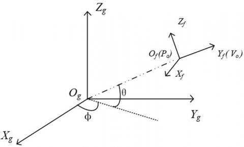
As shown in Figure 1, the formation coordinate system (OfXfYfZf) was defined as a Cartesian coordinate system, in which the origin Of lies at the center po of all UAVs in the formation, the axis OfYf pointing to the mean velocity vo of all UAVs in the formation, the axis OfXf parallel to the horizontal plane XgOgYg in the NED system, and the axis OfZf vertical to the horizontal plane XfOfYf in the formation coordinate system. In addition, φ was defined as the pitch angle of vo in the NED system, and θ as the angle between the projection of vo on the horizontal plane XgOgYg and the axis OgXg. In the formation coordinate system, the pattern of UAV formation can be derived from the ideal positions of the UAVs: $R(t)=\left\{p_{1}^{r}(t), p_{2}^{r}(t), \cdots, p_{N}^{r}(t)\right\}$.
Figure 1. The formation coordinate system
For the flight controller to control the formation, it is necessary to identify the ideal positions of the UAVs in the NED system. To this end, the coordinates of the formation should be transformed from the formation coordinate system to the NED system:
$C=\operatorname{RotaZ} \cdot \operatorname{RotaX}=\left[\begin{array}{ccc}{\cos \theta} & {\sin \theta} & {0} \\ {-\sin \theta} & {\cos \theta} & {0} \\ {0} & {0} & {1}\end{array}\right] \cdot\left[\begin{array}{ccc}{1} & {0} & {0} \\ {0} & {\cos \varphi} & {-\sin \varphi} \\ {0} & {\sin \varphi} & {\cos \varphi}\end{array}\right]$ (6)
Through the above conversion matrix, the NED coordinates of the ideal position of the formation can be obtained as:
$p_{i}^{d}(t)=C \cdot p_{i}^{r}(t)+p_{o}(t)$ (7)
Therefore, the real-time target position of each UAV in the NED system can be described as $D(t)=\left\{p_{1}^{d}(t), p_{2}^{d}(t), \cdots, p_{N}^{d}(t)\right\}$.
3.1 Trajectory prediction under uncertainties based on reachable set
Currently, the future trajectories of obstacles are generally predicted under linear motion assumption. The obstacle is assumed to fly at a constant speed along a straight line. Then, the future position of the obstacle in a time horizon can be deduced based on the current velocity. This approach applies to the forecast of future trajectories, if the obstacle has little change in motion state in the short term. Nevertheless, a moving obstacle cannot fly along a straight line in the long run. The pilot may change the course, and the obstacle may deviate from the planned trajectory under the wind.
Considering the uncertainty in the future trajectories of moving obstacles, this paper decides to predict the possible future motion states of an obstacle with reachable set, rather than linear prediction. The reachable set refers to the scope of region that can be reached by the obstacle in the next time horizon, under its own kinematic constraints (maximum turning radius and maximum turning velocity). Once the future trajectories of the obstacle are predicted based on the reachable set, the conflicts can be detected by judging whether the UAV trajectory intersects with reachable region of the obstacle. For noncooperative obstacles, this detection approach is much more robust than the linear prediction.
3.1.1 Reachable set on 2D plane
Suppose the obstacle flies according to Dubin’s car model. Then, the obstacle flies at a constant velocity and faces a limit on the maximum turning velocity:
$v=$ Const
$\varphi \leq w_{\max }$ (8)
where, v is the horizontal velocity of the obstacle; φ is the heading angle (φmax is the upper limit of the steering angle); wmax is the maximum turning angle of the obstacle corresponding to the minimum turning radius ρ=v⁄wmax. For a given time horizon, the allowable turning velocity of the obstacle falls in [-wmax, wmax]. This produces a set of allowable trajectories, i.e. the reachable set RSxy. The reachable set RSxy is bounded by S1,2,3,4(θ,t) and S5. Among them, S1,2(θ,t) can be respectively expressed as:
$S_{1}(\theta, t)=\left[\begin{array}{c}{-\rho(1-\cos \theta)+(v t+\rho \theta+r) \sin \theta} \\ {-\rho \sin \theta+(v t+\rho \theta+r) \cos \theta}\end{array}\right]$ (9)
$S_{2}(\theta, t)=\left[\begin{array}{c}{\rho(1-\cos \theta)+(v t-\rho \theta+r) \sin \theta} \\ {\rho \sin \theta+(v t-\rho \theta+r) \cos \theta}\end{array}\right]$ (10)
The domains of S1,2(θ,t) can be respectively described as:
$S_{1}: \max \left(-\varphi_{\max },-\pi\right) \leq \theta \leq 0$ (11)
$S_{2}: 0 \leq \theta \leq \min \left(\varphi_{\max }, \pi\right)$ (12)
Similarly, S3,4(θ,t) can be respectively expressed as:
$S_{3}(\theta, t)=S_{1}\left(-\varphi_{\max }, t\right)+\left[\begin{array}{l}{r \sin \theta} \\ {r \cos \theta}\end{array}\right]$ (13)
$S_{4}(\theta, t)=S_{2}\left(\varphi_{\max }, t\right)+\left[\begin{array}{l}{r \sin \theta} \\ {r \cos \theta}\end{array}\right]$ (14)
The domains of S3,4(θ,t) can be respectively described as:
$S_{3}:-\pi \leq \theta \leq-\varphi_{\max }$ (15)
$S_{4}: \cdot \varphi_{\max } \leq \theta \leq \pi$ (16)
where, θ is the normal unit vector of each point. The normal unit vector of point (x,y) is $\vec{n}$=(nx, ny),θ=atan2(nx, ny). Under the given minimum turning radius ρ, maximum turning velocity v, safe radius r and next time horizon t, the derivation process of S1,2,3,4(θ,t) was detailed [29]. S5(t) is the horizontal segment linking up the bottom of S1,2,3,4.
According to formulas (9), (10), (13) and (14), Wmax, V, t, ρ and r were set to 0.013/s, 4 m/s, 10 s, 307.69 m and 3 m, respectively. Then, the boundaries of the reachable set RSxy, i.e. S1,2,3,4(θ,t) and S5, are displayed in Figure 2 below.
Figure 2. The boundaries of the reachable set
If φmax>π, then S3,4 are no longer boundaries of RSxy. In this case, the two boundaries should be replaced by S3(-π,t) and S4(π,t) or by S1(-π,t) and S2(π,t), depending on which pair of curves satisfy θ=±π at time t.
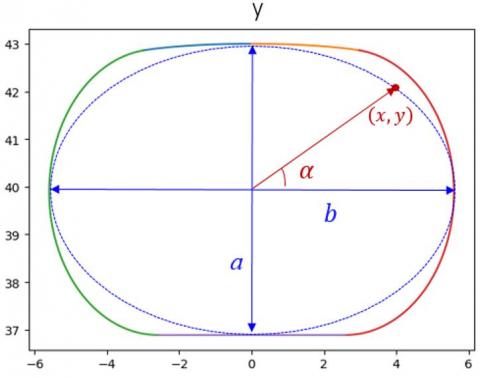
For convenience, the region enclosed by the boundaries of RSxy was approximated as an ellipse (Figure 3), where the length of the major axis a is roughly the maximum lateral distance between S3 and S4 and the length of the minor axis b is roughly the maximum horizontal distance between S1,2 and S5. In this way, the elliptical reachable set $R S_{x y}^{e l l i}$ on the 2D plane xy can be expressed as:
$\left\{\begin{array}{l}{x=a \cos \alpha} \\ {y=b \sin \alpha}\end{array}\right.$ (17)
where, α is the angle between any boundary point (x, y) of the elliptical reachable set $R S_{x y}^{e l l i}$ and the x axis, α∈(0, 2π).
Figure 3. The elliptical reachable set on the 2D plane
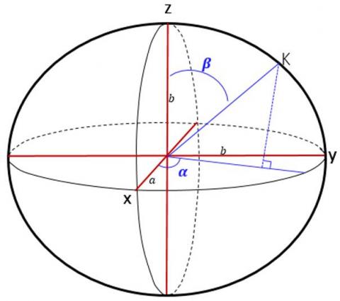
3.1.2 Reachable set in 3D space
When the obstacle is moving in a 3D space, the reachable set can be approximated as an ellipsoid both on plane xy and plane xz. Suppose the ellipsoid on plane xz has the same major and minor axes as that on plane xy, that is, the lengths of major and minor axes are a and b, respectively. As for plane yz, the reachable set can be roughly considered as a circle, whose diameter equals the length of the major axis a. Then, the entire reachable region in the 3D space can be approximated as an ellipsoid (Figure 4). Let k(x,y,z) be a point on the ellipsoid $R S_{x y z}^{e l l i}$. The 3D ellipsoidal reachable set $R S_{x y z}^{e l l i}$ can be defined as:
$x=a \cos \alpha \sin \beta$
$y=b \sin \alpha \sin \beta$
$z=b \cos \beta$ (18)
where, α is the angle between the projection of the normal unit vector of k(x,y,z) on plane xy and the x axis, α∈[0,2π); β is the angle between the normal unit vector of k(x,y,z) and its projection on plane x-z, β∈[0,π].
Figure 4. The 3D ellipsoidal reachable set
3.2 Two-layer safe separation management based on improved APF
The APF method has received extensive attention, because of its fast speed, simple expression and physical significance. In this method, it is assumed that the trajectory of a robot depends on the forces in the virtual potential field: the attractive force from the destination that pulls the robot towards the destination, and the repulsive force on the obstacle that pushes the robot away from the obstacle and threat source. In the virtual potential field, a path can be set up to connect the origin and the destination along the direction of the resultant force of the attractive force and the repulsive force. In this paper, the APF method is improved and adopted for the aircrafts in the UAV formation to realize the safe separation control and obstacle avoidance.
3.2.1 Attractive force
Under the attractive force of the APF, the UAVs move from the original positions to the preset positions of the formation, forming the required formation pattern. The attractive force can be divided into position attractive force Fp and velocity attractive force Fv. The former force is mainly related to the UAV position P. It drags the UAV to the preset position in the formation. The latter force mainly depends on the current velocity of the UAV. This force ensures that all UAVs in the formation fly at the same velocity. The position attractive force and velocity attractive force of UAV i can be respectively expressed as:
$F_{p}^{i}(t)=K_{g}\left(p_{g}-p_{o}(t)\right)+K_{p}\left(p_{i}^{d}(t)-p_{i}(t)\right)$ (19)
$F_{v}^{i}(t)=K_{v}\left(v_{i}^{d}(t)-v_{i}(t)\right)$ (20)
where, K is the weight coefficient; pg is the destination of the entire formation, a key point on the planned trajectory.
When a UAV flies towards the destination, it is continuously subjected to the acceleration generated by the resultant force. As a result, the UAV may still fly at a high velocity even if it comes close to the destination. Chances are that the UAV might fly over the destination. Since the attractive force always points towards the destination, the UAV will eventually oscillate repeatedly about the destination. This phenomenon often occurs when a UAV tries to return to the planned trajectory after successful collision avoidance. To weaken the oscillation, a damping force F pointing to the opposite direction of velocity can be introduced:
$F_{d a m p}^{i}(t)=-K \cdot v_{i}(t)$ (21)
Then, the overall attractive force can be depicted as:
$F_{a t t}^{i}(t)=F_{p}^{i}(t)+F_{v}^{i}(t)+F_{d a m p}^{i}(t)$ (22)
3.2.2 Repulsive force
The repulsive force keeps the UAVs outside the safe distance. In this paper, the repulsive force of UAV i consists of two parts: the repulsive force $F_{r e p_{-} o b s}^{i}$ that keeps the safe distance from a noncooperative obstacle, and the repulsive force $F_{r e p{-i n n e r}}^{i}$ that keeps the safe distance between cooperative UAVs in the formation.
(1) Repulsive force between a UAV and a noncooperative obstacle. The reachable region of an obstacle after the time horizon Ks can be computed by formula (18). Meanwhile, the position of the UAV in Ks can be determined based on its current position and velocity. If the UAV will enter the reachable region of the obstacle in Ks, the UAV should perform collision avoidance maneuvers under the traditional distance-based potential field force. Otherwise, the UAV should fly forward in the original motion state.
Based on the reachable region, the repulsive force between UAV i and a noncooperative obstacle can be calculated by:
$F_{r e p_{-} o b s}^{i}=\left\{\begin{array}{cc}{K_{o b s} \cdot\left(\frac{1}{r_{s a f e}^{o b s}-o b s}-\frac{1}{\|\vec{d}\|}\right) \frac{\vec{d}}{\|\vec{d}\|},} & {\text { for }\|\vec{d}\|<r_{s a f e}^{o b s}} \\ {0,} & {\text { otherwise }}\end{array}\right.$ (23)
where, $\vec{d}$ is the distance from the UAV to the reachable region of the obstacle; $r_{\text {safe }}^{\text {obs }}$ is the safe distance between the UAV and the reachable region of the obstacle. If $\vec{d}$ is smaller than $r_{\text {safe}}^{o b s}$, then the repulsive force will act on the UAV to push it away from the reachable region. As shown in Figure 5, $r_{\text {safe}}^{o b s}$ is dependent on the size of the reachable region and the boundaries of the safe region of the UAV:
$r_{s a f e}^{o b s}=\left\{\begin{array}{c}{r_{s a f e}^{\operatorname{min}}+r_{e l l i}+K \cdot v_{i} \cdot \cos \delta, i f \delta \in\left[0, \frac{\pi}{2}\right]} \\ {r_{s a f e}^{\min }+r_{e l l i}, e l s e}\end{array}\right.$ (24)
where, δ is the angle between the velocity direction of the UAV and the connecting line between the UAV and the obstacle; vi is the UAV velocity; vi⋅cosδ is the component of the UAV velocity along the connecting line between the UAV and the center of the reachable region, i.e. the approaching velocity between the UAV and the obstacle; $r_{\text {safe }}^{\text {outer }}=K \cdot v_{i}(t) \cdot \cos \delta$ is the outer boundaries of the UAV’s safe region; K is the time horizon depending on the UTM’s regulaiton capacity; $r_{\text {safe}}^{\min }$ is the minimum safe distance (any distance smaller than $r_{\text {safe}}^{\min }$ will lead to collision); relli is the distance from the ellipsoid center to ellipsoid surface along the connecting line between the UAV and the center of the reachable region. The center to surface distance of the ellipsoid can be computed by:
$r_{\text {elli }}=\sqrt{(a \sin \beta \cos \alpha)^{2}+(b \sin \beta \sin \alpha)^{2}+(b \cos \beta)^{2}}$ (25)
Figure 5. Safe distance between a UAV and an obstacle
(2) Repulsive force between cooperative UAVs in the formation. Traditionally, the repulsive force is only related to relative position. When the UAV moves at a high velocity, such a repulsive force cannot guarantee successful avoidance of collision. To adapt to the real-time dynamic requirements of the UAV formation, this paper modifies the traditional function of the repulsive force. The UAV velocity was included as an influencing factor of the repulsive force. In the revised function, both the direction and magnitude of velocity can be adjusted by the repulsive force. In other words, the repulsive force between cooperative UAVs in the formation Frep_inner depends both on relative position and the direction of relative velocity. Let $F_{r e p}^{i j}$ be the repulsive force of UAV j to UAV i. Then, the modified function of the repulsive force can be expressed as:
$F_{_{rep\_inner//}}^{{}}=\left\{ \begin{matrix} K\cdot (\frac{1}{r_{_{safe}}^{inner}}-\frac{1}{\left\| {\vec{d}} \right\|})\cdot ({{{\vec{v}}}_{j}}-{{{\vec{v}}}_{i}})\cdot \cos \delta ,\text{ }for\text{ }\left\| {\vec{d}} \right\|<r_{_{safe}}^{inner} \\ 0,otherwise \\\end{matrix} \right.$ (26)
$F_{_{rep\_inner\bot }}^{{}}=\left\{ \begin{matrix} K\cdot (\frac{1}{r_{_{safe}}^{inner}}-\frac{1}{\left\| {\vec{d}} \right\|})\frac{\vec{d}\cdot \left\| {{{\vec{v}}}_{j}}-{{{\vec{v}}}_{i}} \right\|\cos \delta }{\left\| {\vec{d}} \right\|}-{{F}_{rep\_inner//}},\text{ }for\text{ }\left\| {\vec{d}} \right\|<r_{_{safe}}^{inner} \\ 0,otherwise \\\end{matrix} \right.$(27)
$F_{r e p_{-} i n n e r}^{i j}=\alpha F_{r e p_{-} i n n e r \perp}+\beta F_{r e p_{-} i n n e r / /}$ (28)
where, α and β are weight factors; $\left\|\vec{v}_{j}-\vec{v}_{i}\right\| \cos \delta$ is the approaching velocity between UAVs i and j (the greater the approaching velocity, the larger the repulsive force); $\vec{v}_{j}$ is the obstacle velocity during collision avoidance; $r_{\text {safe}}^{\text {inner}}$ is the safe distance between a UAV and its surrounding UAVs. If two UAVs are closer than the $r_{\text {safe }}^{\text {inner }}$, the repulsive force will emerge to keep the two UAVs outside the safe distance. Considering the velocity states of relevant UAVs, the $r_{\text sa f e}^{\text {inner }}$ can be defined as:
$r_{\text {safe}}^{\text {inner}}=\left\{\begin{array}{c}{2 \cdot r_{\text {safe}}^{\min }+K_{\text {safe}} \cdot\left(v_{i}-v_{j}\right) \cdot \cos \delta, \text {if } \delta \in\left[0, \frac{\pi}{2}\right]} \\ {2 \cdot r_{\text {safe}}^{\min }, \text {else}}\end{array}\right.$ (29)
When two UAVs are approaching each other, the increases with the relative velocity.
If UAV i senses N UAVs in the formation to be avoided from at time t, then the total repulsive force needed to complete the collision avoidance can be described as:
$F_{r e p_{-} i n n e r}^{i}=\sum_{j}^{N} F_{r e p_{-} i n n e r}^{i j}$ (30)
The total repulsive force acting on UAV i can be determined as:
$F_{r e p}^{i}=F_{r e p_{-} o b s}^{i}+F_{r e p_{-} i n n e r}^{i}$ (31)
According to the states of each UAV and the information of the airspace, the resultant force of the potential field can be obtained as:
$F_{\text {total}}^{i}=F_{a t t}^{i}+F_{r e p}^{i}$ (32)
This section simulates the encounter between a three-UAV formation and a noncooperative obstacle. First, the 3D reachable region of the moving obstacle was visually presented. After that, the authors verified whether our method can effectively keep a UAV in safe distance from other UAVs and the obstacle, minimize the deviation of the collision-free trajectory from the planned trajectory, and mitigate the violent changes in UAV velocity and acceleration.
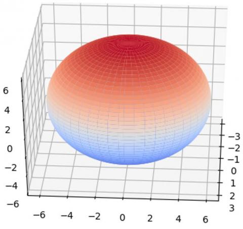
4.1 Reachable region
Figure 6 shows the ellipsoidal reachable region of the moving obstacle in the time horizon of 10s. As shown in the figure, planes xz and xy are ellipses, while plane zy is a circle. The moving obstacle may appear in any point in the region after 10 s.
Figure 6. The ellipsoidal reachable region of the noncooperative obstacle
4.2 Encounter scenes
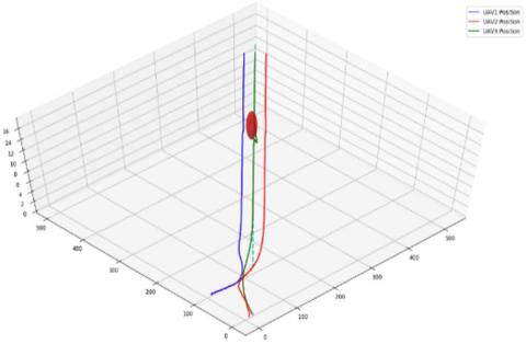
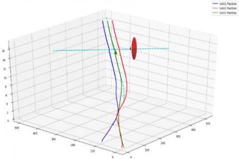
In the 3D airspace (Figure 6), three UAVs set out from different positions, each with a unique acceleration and velocity. As shown in Figure 7(a), the three UAVs soon reached basically the same direction and magnitude of velocity, and flied at relatively fixed positions, indicating that the formation had been established. The formation pattern is $x_{1}^{r}$=[-20,0,0,0,0,0]T, $x_{2}^{r}$ =[20,0,0,0,0,0]T, and $x_{3}^{r}$=[0,0,0,0,0,0]T. Meanwhile, an obstacle (the red dot) flied across the trajectories of the three UAVs. The reachable region and trajectory of the obstacle are respectively displayed as a red ellipsoid and a blue dotted line. When the three UAVs encountered the obstacle, the UAV3 at the middle detected the entry into the reachable region of the obstacle, and performed collision avoidance maneuvers, without violating the safe distance with the other two UAVs.
(a) Before conflict
(b) Conflict resolution
(c) After resolution
Figure 7. Collision avoidance process between the UAV formation and the noncooperative obstacle
4.3 Safety analysis
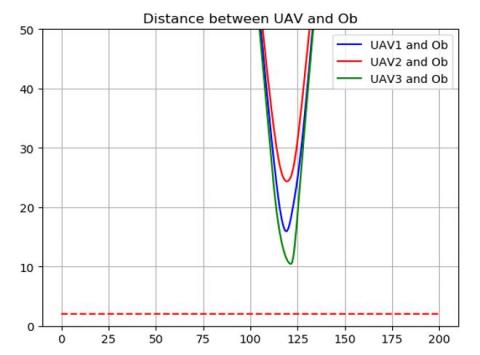
Figure 8 shows the safe distance between each UAV and the obstacle in the conflict resolution process. The red dotted line stands for the collision distance. Obviously, the safe distances between all three UAVs and the obstacle were greater than the collision distance throughout the process. This means all UAVs in the formation successfully avoided colliding into the obstacle. It can also be seen that the UAV formation maintained a large safe distance from the obstacle.
The real-time distances between the three UAVs are plotted in Figure 9. It can be seen that, at around 120s, UAV3 moved closer to UAV2 and away from UAV1, when the UAV took collision avoidance measures. This is because UAV3 moved towards UAV2 during conflict resolution. In addition, the distances between the three UAVs were greater than the collision distance, indicating that no conflict occurred between them.
Figure 8. Variation in safe distance between each UAV and the obstacle
Figure 9. Variation in safe distances between UAVs in the formation
4.4 Performance comparison
To verify its stability and safety, the proposed method, i.e. the safe distance management based on trajectory prediction, was compared with the safe distance management based on motion state [23] and the traditional APF method, in terms of the deviation of conflict resolution trajectory from the planned trajectory, and the fluctuation of velocity and acceleration. The safe distance management based on motion state was referred to as the previous method, because it was proposed previously by the authors.
4.4.1 Comparison of trajectory deviation
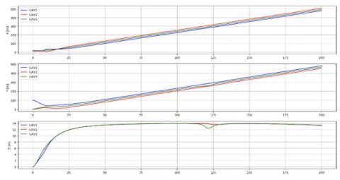
As shown in Figures 10 and 11, the UAV formation encountered the obstacle after flying for 120s. In the formation, UAV3 and UAV2 moved away from the planned trajectories after the encounter. The trajectory deviation was mainly observed in the vertical direction (z axis). The trajectory deviation of UAV3 was greater than that of UAV2. The trajectory deviation of our method (Figure 10) was obviously smaller than the previous method (Figure 11). Therefore, our method could generate relatively stable conflict resolution trajectories, making the collision avoidance maneuvers gentle and elegant, with limited impact on nearby traffic in the airspace.
In Figure 10, UAV3 started to move away from the planned trajectory at 103 s, successfully resolved the conflict at 122 s, and returned to the planned trajectory at 130 s. The entire conflict resolution took 27s. In Figure 11, the corresponding time points were 110 s, 121s and 148s, and the conflict was resolved fully in 38 s. Compared with that of the previous method, the conflict resolution by our method takes effect early, restores the planned path rapidly, and ensures the safety of the UAVs.
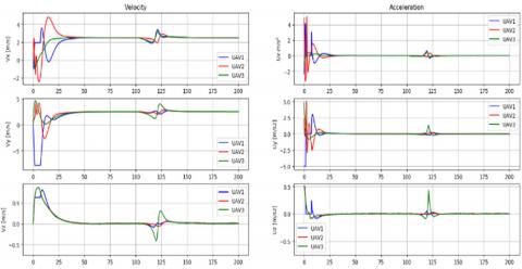
4.4.2 Comparison of velocity and acceleration fluctuations
In 102 s, the three UAVs encountered the obstacle and started to make conflict resolution maneuvers. The velocity and acceleration fluctuations of our method, the previous method and the traditional APF method are displayed in Figures 12-14, respectively. Judging by the acceleration fluctuations, UAV3 mainly maneuvered along the vertical direction (z axis), with limited fluctuations in horizontal velocity and acceleration. By the traditional APF method, sudden fluctuations appeared on the velocity and acceleration in the vertical direction, which may surpass the physical constraints of the UAV, making the maneuvers inexecutable. By contrast, the velocity and acceleration by our method and the previous method fluctuated rather gently in conflict resolution, and our method boasts the gentlest changes of velocity and acceleration in the vertical direction.
Figure 10. Trajectory deviations of our method
Figure 11. Trajectory deviations of the previous method
Figure 12. Velocity and acceleration fluctuations of our method
Figure 13. Velocity and acceleration fluctuations of the previous method
Figure 14. Velocity and acceleration fluctuations of the traditional APF method
Focusing on uncertain, crowded airspaces, this paper puts forward a separation management method based on trajectory prediction, aiming to maintain the safe distance between each UAV and the other UAVs in the formation, and between each UAV and a noncooperative obstacle. Firstly, the region that a noncooperative obstacle may fly to within a time horizon was predicted based on the reachable set, for the future trajectory of the obstacle is uncertain under the effects of pilot reaction, wind and other external factors. Next, the possibility of conflict was judged according to the reachable region of the noncooperative obstacle, and the affected UAVs in the formation need to perform collision avoidance maneuvers by the distance-based APF method. In this way, the conflict resolution measure is taken early, maximizing the safety of the UAVs, and the UAVs could avoid the risk of collision by moving slightly away from the planned trajectory. Since a UAV in conflict resolution inevitably affects the surrounding UAVs, this paper designs the APF method based on relative motion state to generate the collision avoidance trajectory. In our method, the approaching velocity between the UAVs is positively correlated with the safe distance and the deviation from the planned trajectory; the UAVs in the formation could adjust their safe distances in real time, and adapt to the flexibly changing patterns of the formation. The simulation results show that our method can effectively maintain the safe distance and prevent the collisions between UAVs and between UAVs and a noncooperative obstacle, and outperform the existing methods in safety, stability and robustness.
This work is supported by the State Key Program of National Natural Science of China (Grant No. 71731001).
[1] Jiang, T., Geller, J., Ni, D., Collura, J. (2016). Unmanned aircraft system traffic management: Concept of operation and system architecture. International Journal of Transportation Science and Technology, 5(3): 123-135. https://doi.org/10.1016/j.ijtst.2017.01.004
[2] Kopardekar, P., Rios, J., Prevot, T., Johnson, M., Jung, J. Robinson III, J.E., (2016). UAS traffic management (UTM) concept of operations to safely enable low altitude flight operations. 16th AIAA Aviation Technology, Integration, and Operations Conference, Washington, D.C. https://doi.org/10.2514/6.2016-3292
[3] Kuchar, J.K., Yang, L.C. (2000). A review of conflict detection and resolution modeling methods. IEEE Transactions on Intelligent Transportation Systems, 1(4): 179-189. https://doi.org/10.1109/6979.898217
[4] Jenie, Y.I., Van Kampen, E.J., Ellerbroek, J., Hoekstra, J.M. (2017). Taxonomy of conflict detection and resolution approaches for unmanned aerial vehicle in an integrated airspace. IEEE Transactions on Intelligent Transportation Systems, 18(3): 558-567. https://doi.org/10.1109/TITS.2016.2580219
[5] Zhang, X., Du, Y., Gu, B., Xu, G., Xia, Y. (2018). Survey of safety management approaches to unmanned aerial vehicles and enabling technologies. Journal of Communications and Information Networks, 3(4): 1-14. https://doi.org/10.1007/s41650-018-0038-x
[6] Aggarwal, S., Kumar, N. (2020). Path planning techniques for unmanned aerial vehicles: A review, solutions, and challenges. Computer Communications, 149: 270-299. https://doi.org/10.1016/j.comcom.2019. 10.014
[7] Song, B., Qi, G., Xu, L. (2019). A survey of three-dimensional flight path planning for unmanned aerial vehicle. 2019 Chinese Control And Decision Conference (CCDC), Nanchang, China, China. https://doi.org/10.1109/ccdc.2019.8832890
[8] Liu, Y., Bucknall, R. (2018). A survey of formation control and motion planning of multiple unmanned vehicles. Robotica, 36(7): 1019-1047. https://doi.org/10.1017/S0263574718000218
[9] Phuong, P.D., Recchiuto, C.T., Sgorbissa, A. (2018). Real-time path generation and obstacle avoidance for multirotors: A novel approach. Journal of Intelligent and Robotic Systems: Theory and Applications, 89(1-2): 27-49. https://doi.org/10.1007/s10846-017-0478-9
[10] Seo, J., Kim, Y., Kim, S., Tsourdos, A. (2017). Collision avoidance strategies for unmanned aerial vehicles in formation flight. IEEE Transactions on Aerospace and Electronic Systems, 53(6): 2718-2734. https://doi.org/10.1109/TAES.2017.2714898
[11] Yang, J., Yin, D., Shen, L. (2017). Reciprocal geometric conflict resolution on unmanned aerial vehicles by heading control. Journal of Guidance, Control, and Dynamics, 40(10): 1-13. https://doi.org/10.2514/1.G002607
[12] Lin, Y., Saripalli, S. (2017). Sampling-based path planning for UAV collision avoidance. IEEE Transactions on Intelligent Transportation Systems, 18(11): 3179-3192. https://doi.org/10.1109/TITS.2017.2673778
[13] Liang, X., Meng, G., Xu, Y., Luo, H. (2018). A geometrical path planning method for unmanned aerial vehicle in 2D/3D complex environment. Intelligent Service Robotics, 11(3): 301-312. https://doi.org/10.1007/s11370-018-0254-0
[14] Li, J., Deng, G., Luo, C., Lin, Q., Yan, Q., Ming, Z. (2016). A hybrid path planning method in unmanned air/ground vehicle (UAV/UGV) cooperative systems. IEEE Transactions on Vehicular Technology, 65(12): 9585-9596. https://doi.org/10.1109/TVT.2016.2623666
[15] Wang, G.G., Chu, H.E., Mirjalili, S. (2016). Three-dimensional path planning for UCAV using an improved bat algorithm. Aerospace Science and Technology, 49: 231-238. https://doi.org/10.1016/j.ast.2015.11.040
[16] Song, B., Wang, Z., Sheng, L. (2016). A new genetic algorithm approach to smooth path planning for mobile robots. Assembly Automation, 36(2): 138-145. https://doi.org/10.1108/aa-11-2015-094
[17] Shao, Z., Yan, F., Zhou, Z., Zhu, X. (2019). Path planning for multi-UAV formation rendezvous based on distributed cooperative particle swarm optimization. Applied Sciences (Switzerland), 9(13): 2621. https://doi.org/10.3390/app9132621
[18] Yang, J., Yin, D., Niu, Y., Zhu, L. (2016). Cooperative conflict detection and resolution of civil unmanned aerial vehicles in metropolis. Advances in Mechanical Engineering, 8(6): 1-16. https://doi.org/10.1177/1687814016651195
[19] Radmanesh, M., Kumar, M. (2016). Flight formation of UAVs in presence of moving obstacles using fast-dynamic mixed integer linear programming. Aerospace Science and Technology, 50: 149-160. https://doi.org/10.1016/j.ast.2015.12.021
[20] Chang, K., Xia, Y., Huang, K. (2016). UAV formation control design with obstacle avoidance in dynamic three-dimensional environment. Springer Plus, 5: 1124. https://doi.org/10.1186/s40064-016-2476-y
[21] Zhu, L., Cheng, X., Yuan, F.G. (2016). A 3D collision avoidance strategy for UAV with physical constraints. Measurement: Journal of the International Measurement Confederation, 77: 40-49. https://doi.org/10.1016/j.measurement.2015.09.006
[22] Sun, J., Tang, J., Lao, S. (2017). Collision avoidance for cooperative UASs with optimized artificial potential field algorithm. IEEE Access, 5: 18382-18390. https://doi.org/10.1109/ACCESS.2017.2746752
[23] Nie, Z.L., Zhang, X.J., Guan, X.M. (2017). UAV formation flight based on artificial potential force in 3D environment. 2017 29th Chinese Control and Decision Conference (CCDC), Chongqing, China. https://doi.org/10.1109/CCDC.2017.7979468
[24] Sun, J., Tang, J., Lao, S. (2017). Collision avoidance for cooperative UAVs with optimized artificial potential field algorithm. IEEE Access, 5: 18382-18390. https://doi.org/10.1109/ACCESS.2017.2746752
[25] Bayat, F., Najafinia, S., Aliyari, M. (2018). Mobile robots path planning: Electrostatic potential field approach. Expert Systems with Applications, 100: 68-78. https://doi.org/10.1016/j.eswa.2018.01.050
[26] Zhou, Z., Wang, J., Zhu, Z., Yang, D., Wu, J. (2018). Tangent navigated robot path planning strategy using particle swarm optimized artificial potential field. Optik, 158: 639-651. https://doi.org/10.1016/j.ijleo.2017.12.169
[27] Zhang, J., Yan, J., Zhang, P. (2018). Fixed-wing UAV formation control design with collision avoidance based on an improved artificial potential field. IEEE Access, 6: 78342-78351. https://doi.org/10.1109/ACCESS.2018.2885003
[28] Zhu, X., Liang, Y., Yan, M. (2019). A flexible collision avoidance strategy for the formation of multiple unmanned aerial vehicles. IEEE Access, 7: 140743-140754. https://doi.org/10.1109/access.2019.2944160
[29] Lin, Y., Saripalli, S. (2015). Collision avoidance for UAVs using reachable sets. 2015 International Conference on Unmanned Aircraft Systems (ICUAS), Denver, CO, USA. https://doi.org/10.1109/ICUAS.2015.7152295