Maheshwar Pathak![]() | Pratibha Joshi*
| Pratibha Joshi*![]() | Kottakkaran Sooppy Nisar
| Kottakkaran Sooppy Nisar![]()
© 2024 The authors. This article is published by IIETA and is licensed under the CC BY 4.0 license (http://creativecommons.org/licenses/by/4.0/).
OPEN ACCESS
Ceramic coatings work as a tool to protect the material from excessive heat or any other rough exposure. Composites with coatings of functionally graded materials are becoming very popular with their very useful thermo-mechanical properties. In this study, a steady state thermal analysis is performed on a composite having two layers, one with the homogeneous substrate and the second is FGM coating under high-temperature exposure of the top of the surface. The numerical examples taken are having cracks along interfaces that produce discontinuities in temperature as well as flux. A decomposed immersed interface method is applied for obtaining the solution of the considered numerical examples which incorporates various types of discontinuity along the crack.
composite structure, immersed interface method, steady state heat conduction
In many scientific and industrial applications, heat transfer in a composite multilayered system is studied. Thermal barrier coating has been always used on important structures such as aircraft engines and stationary gas turbines [1-3] to protect them from high heat. The coating is chosen depending upon the environment and the structure which needs the protection. For developing a well-protected structure, a detailed study of reliability, efficiency, and toughness of coating under a harsh outer environment is required. Functionally graded materials (FGMs) are multifunctional materials [4], which are specifically designed compositions for the purpose of maintaining variations in thermal, structural, or functional properties. FGM coatings on a homogeneous substrate can protect all the crucial properties of the base if designed properly.
In this study, a thermal analysis is performed on a multilayered composite composed of two layers. One layer is of a homogeneous substrate and the second layer is the FGM coating. The top of the surface is exposed to high temperatures. The contact between the FGM layer and substrate is also not perfect and leads to a crack where discontinuities occur in temperature and flux. The standard methods fail on a multilayered composite with discontinuities in solution and its derivatives as the jumps along the interface need to be addressed.
Many numerical methods [5-9] are designed for heat transfer problems [10-15] in a composite medium with one or more interfaces. Finite difference method-based approach is used to solve the heat transfer model in multilayered composite cylinders in the study of Alaa et al. [16] and for the analysis of transient heat transfer in a phase change composite thermal energy storage (PCC-TES) system arising in air conditioning applications [17]. In the study of Skerget et al. [18], a combination of boundary element method and finite difference method is used study heat transfer in a multilayered composite pipeline. In [19], hybrid flux finite element metho d(HF-FEM) and hybrid thermal stress finite element method (HTSFEM) based on 3D polyhedron-octree is applied to simulate the steady-state heat conduction and thermal stress of particle-reinforced composites. Ibouroi et al. [20] introduce and evaluate a numerical method based on separation of variable method and Green’s function for calculating the thermal behavior of composite beams exposed to heat sources positioned at any location and exhibiting varying temporal patterns. In the study of Zhai et al. [21], an innovative numerical framework that merges the multiscale asymptotic approach with Laplace transformation is presented for the solution of the three-dimensional dual-phase-lagging equation arising in heat conduction in composite materials. The common disadvantages in most of the existing methods for the study of heat transfer in composite systems is that they ignore any kind of discontinuities along the interface. For such applications, a numerical method is necessary that can handle discontinuities while preserving accuracy and simplicity.
Berthelsen [15] proposes a decomposed immersed interface method (DIIIM) in which the difference stencil is corrected on the right-hand side only in order to ensure the resulting linear system can be solved by traditional solvers. This correction term is evaluated direction-wise and can be improved by iterative schemes. In this study, DIIIM is applied in finding the temperature distribution in a FGM coated two-layered composite whose top is exposed to very high temperature. In general, it is seen that in modelling any phenomena in a composite layered system, the contact is shown perfect due to the unavailability of efficient methods to deal with discontinuities along the interface. DIIIM can deal with various kinds of discontinuities by incorporating jumps along the interface into the standard finite difference scheme. Thus, it is best suited for heat conduction problems in multilayer composites with imperfect contact.
The rest of the paper is divided into four more sections. The second section explains the mathematical model of the considered problem. The third section describes the decomposed immersed interface method (DIIM) in detail which is used for determining the thermal profile in the current study. In the fourth section few numerical examples are taken for evaluation of their temperature distribution. In the last section the conclusion of the current study is mentioned.
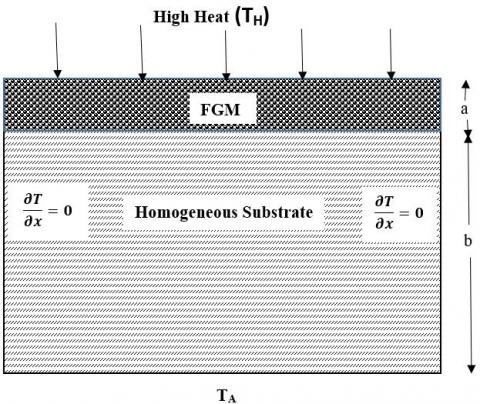
In the present study steady-state heat conduction in a two layered composite (see Figure 1) of $1 \mathrm{~m} \times 1 \mathrm{~m}$ dimension is considered where top layer is a FGM coating and bottom layer is of a homogeneous substrate. The coating is relatively thin in comparison to the bottom layer.
Figure 1. FGM-coated composite
Let $K_1$ be the thermal conductivity of the substrate and $K_2$ be the thermal conductivity of FGM coating. Let $T(x, y)$ be the temperature and $f(x, y)$ be the source term of the considered composite at an arbitrary point $(x, y)$. The governing equation of steady state heat conduction in the composite is as follows:
$K \frac{\partial^2 T}{\partial x^2}+K \frac{\partial^2 T}{\partial y^2}=f(x, y)$
where,
$K=\left\{\begin{array}{ll}K_1 & y<b \\ K_2 & y>b\end{array}\right.$ and $f(x, y)= \begin{cases}f_1(x, y) & y<b \\ f_2(x, y) & y>b\end{cases}$
The bottom of the composite is at room temperature $T_A$. The left and right sides of the composite are considered perfectly insulated and the top of the composite is at high-temperature $T_H$. Hence the boundary condition can be formulated as:
$\begin{array}{ll}T=T_A, & y=0, x \in[0,1] \\ T=T_H, & y=1, x \in[0,1] \\ \frac{\partial T}{\partial x}=0, & x=0, y \in[0,1] \\ \frac{\partial T}{\partial x}=0, & x=1, y \in[0,1]\end{array}$
The two layers have an interface $\Gamma$ at $y=b$ along the contact is not perfect which leads to various kinds of discontinuities. The jump along the interface $\Gamma$ in any function $g(x, y)$ is defined as
$[g(x, y)]=\lim _{(x, y) \rightarrow \Gamma^{+}} g(x, y)-\lim _{(x, y) \rightarrow \Gamma^{-}} g(x, y)$
Let the jumps in the current cases be
$\begin{gathered}{[T]=A_1} \\ {\left[k \frac{\partial T}{\partial y}\right]=A_2} \\ {\left[k \frac{\partial^2 T}{\partial y^2}\right]=A_3}\end{gathered}$
where, $A_1, A_2$ and $A_3$ can be constants or a function of $x$.
In the current study DIIM [15] is applied to obtain the required temperature distribution as it deals with the discontinuities along the interface without disturbing the standard five-point stencil. Hence the resulting linear system is symmetric and diagonally dominant which can be solved by any standard solver. In this section DIIM is explained in detail.
Suppose we have a domain $\mathrm{R}$ divided into subdomains $R^{+}$and $R^{-}$by an interface $\Gamma$. Let us consider an elliptic boundary value problem
$\frac{\partial}{\partial x}\left(\beta \frac{\partial \theta}{\partial x}\right)+\frac{\partial}{\partial y}\left(\beta \frac{\partial \theta}{\partial y}\right)=w(x, y)$ (1)
Suppose $\beta$ and source term $w$ have jumps across the interface $\Gamma$ which cause jumps in the solution and its derivatives too.
The interface is represented through a smooth auxiliary function $\psi(x, y)$ as
$\psi(x, y)= \pm d$
where, $d$ is the nearest distance to the interface. Using the zero-level set function as an interface.
$\Gamma=\{(x, y) \in R \mid \psi(x, y)=0\}$
Positive sign of $\psi(x, y)$ directs that the point $(x, y)$ is in the $R^{+}$region and negative sign of $\psi(x, y)$ directs that the point $(x, y)$ is in the $R^{-}$region i.e.
$R= \begin{cases}R^{-}, & \psi<0 \\ R^{+}, & \psi>0\end{cases}$
Numerical Discretization: Let a domain be $\mathrm{D}=\left[a_1, b_1\right] \times$ $\left[a_2, b_2\right]$. The uniform grid is structured in the following as
$x_i=a_1+i h, y_j=a_2+j h$
where,
$h=\frac{b_1-a_1}{M}=\frac{b_2-a_2}{N}$ and $0 \leq i \leq M, 0 \leq j \leq N$.
The grid points between which the interface intersects are called irregular points. Regular points are those between which the interface does not intersect. The central finite difference discretization of (1) at regular points is
$\begin{aligned} & \frac{\beta_{i+1 / 2, j}\left(\theta_{i+1, j}-\theta_{i, j}\right)-\beta_{i-1 / 2, j}\left(\theta_{i, j}-\theta_{i-1, j}\right)}{h^2} +\frac{\beta_{i, j+1 / 2}\left(\theta_{i, j+1}-\theta_{i, j}\right)-\beta_{i, j-1 / 2}\left(\theta_{i, j}-\theta_{i, j-1}\right)}{h^2} =w_{i, j}\end{aligned}$ (2)
where, $\quad \theta_{i, j}=\theta\left(x_i, y_j\right), w_{i, j}=w\left(x_i, y_j\right)$ and $\beta_{i+1 / 2, j}=$ $\beta\left(x_i+h / 2, y_j\right)$. At irregular grid points, the right-hand side of Eq. (2) contains a correction term cor$_{i, j}$ designed to make numerical discretization well defined at irregular nodes and disappear at regular nodes. Due to the fact that jump conditions can be decomposed in both directions, this correction term is decomposable dimension-by-dimension. Hence, we define the correction term as
$\operatorname{cor}_{i, j}=\operatorname{cor}_{i, j}^x+\operatorname{cor}_{i, j}^y$
A similar procedure in the y-direction can be followed as we evaluate the correction term in the x-direction. Hence, we have discussed the procedure of evaluating correction term in only $x$-direction.
Let us suppose that interface is situated at $x_{\Gamma}=x_i+\vartheta h$, $\leq \vartheta \leq 1, \vartheta=\frac{\psi_i}{\psi_i-\psi_{i+1}}$ where $x_i$ is an irregular node and $\psi_i=\psi\left(x_i\right)$. First, the numerical discretization of $\theta_x$ is corrected and then the approximation of $\left(\beta \theta_x\right)_x$ is corrected. The first derivative is estimated at the center between $x_i$ and $x_{i+1}$. The correction term of (2) is decided on the basis of the side of $x_{i+1 / 2}$, the interface is located.
Expression of $\theta\left(x_{i+1}\right)$ at $x_{\Gamma}=x_i+\vartheta h$ for the case $\psi_i<$ 0 and $1 / 2<\vartheta \leq 1$ using Taylor's series expansion
$\begin{aligned} & \theta\left(x_{i+1}\right)=\theta\left(x_{\Gamma}+(1-\vartheta) h\right) \\ & =\theta^{+}+\theta_x^{+}(1-\vartheta) h+\frac{1}{2} \theta_{x x}^{+}(1-\vartheta)^2 h^2+O\left(h^3\right) \\ & =\theta^{-}+\theta_x^{-}(1-\vartheta) h+\frac{1}{2} \theta_{x x}^{-}(1-\vartheta)^2 h^2+\operatorname{cor}_1(x, \vartheta)+O\left(h^3\right) \\ & =\theta\left(x_{i+\frac{1}{2}}\right)+\theta_x\left(x_{i+\frac{1}{2}}\right)\left(\vartheta-\frac{1}{2}\right) h+\frac{1}{2} \theta_{x x}\left(x_{i+\frac{1}{2}}\right)\left(\vartheta-\frac{1}{2}\right)^2 h^2 \\ & +\theta_x\left(x_{i+1 / 2}\right)(1-\vartheta) h+\frac{1}{2} \theta_{x x}\left(x_{i+1 / 2}\right)(2 \vartheta-1)(1-\vartheta) h^2 \\ & +\frac{1}{2} \theta_{x x}\left(x_{i+1 / 2}\right)(1-\vartheta)^2 h^2+\operatorname{cor}_1(x, \sigma)+O\left(h^3\right) \\ & =\theta\left(x_{i+\frac{1}{2}}\right)+\theta_x\left(x_{i+\frac{1}{2}}\right) \frac{h}{2}+\frac{1}{2} \theta_{x x}\left(x_{i+\frac{1}{2}}\right)\left(\frac{h}{2}\right)^2+\operatorname{cor}_1(x, \vartheta) +O\left(h^3\right)\end{aligned}$ (3)
Similarly, the expression of $\theta\left(x_i\right)$ at $x_{i+1 / 2}$
$\begin{aligned} \theta\left(x_i\right)=\theta\left(x_{i+1 / 2}\right) & -\theta_x\left(x_{i+1 / 2}\right) \frac{h}{2} +\frac{1}{2} \theta_{x x}\left(x_{i+1 / 2}\right)\left(\frac{h}{2}\right)^2+O\left(h^3\right)\end{aligned}$ (4)
The correction term is evaluated from [3] as
$\operatorname{cor}_1(x, \sigma)=[\theta]+\left[\theta_x\right](1-\vartheta) h+\frac{1}{2}\left[\theta_{x x}\right](1-\vartheta)^2 h^2$
On subtracting (4) from (3)
$\theta\left(x_{i+1 / 2}\right)=\frac{\theta\left(x_{i+1}\right)-\theta\left(x_i\right)}{h}-\frac{\operatorname{cor}_1(x, \vartheta)}{h}+O\left(h^2\right)$
In case of $0<\vartheta \leq \frac{1}{2}$ expanding $\theta\left(x_i\right)$ at $x_{\Gamma}=x_i+\vartheta h$
$\begin{aligned} & \theta\left(x_i\right)=\theta\left(x_{\Gamma}-\vartheta h\right)=\theta^{-}-\theta_x^{-} \sigma h+\frac{1}{2} \theta_{x x}^{-} v^2 h^2+O\left(h^3\right) \\ & =\theta^{+}-\theta_x^{+} \vartheta h+\frac{1}{2} \theta_{x x}^{+} v^2 h^2-\operatorname{cor}_1(x, v)+O\left(h^3\right) \\ & =\theta\left(x_{i+\frac{1}{2}}\right)-\theta_x\left(x_{i+\frac{1}{2}}\right)\left(\frac{1}{2}-\vartheta\right) h+\frac{1}{2} \theta_{x x}\left(x_{i+\frac{1}{2}}\right)\left(\frac{1}{2}-\vartheta\right)^2 h^2 \\ & \quad-\theta_x\left(x_{i+\frac{1}{2}}\right) \vartheta+\frac{1}{2} \theta_{x x}\left(x_{i+\frac{1}{2}}\right)(1-2 \vartheta) \vartheta h^2 \\ & \quad+\frac{1}{2} \theta_{x x}\left(x_{i+\frac{1}{2}}\right) \vartheta^2 h^2-\operatorname{cor}_1(x, \vartheta)+O\left(h^3\right) \\ & =\theta\left(x_{i+1 / 2}\right)-\theta_x\left(x_{i+1 / 2}\right) \frac{h}{2}+\frac{1}{2} \theta_{x x}\left(x_{i+1 / 2}\right)\left(\frac{h}{2}\right)^2-\operatorname{cor}_1(x, \vartheta) +O\left(h^3\right)\end{aligned}$ (5)
Writing expression of $\theta\left(x_{i+1}\right)$ at $x_{i+1 / 2}$
$\begin{gathered}\theta\left(x_{i+1}\right)=\theta\left(x_{i+1 / 2}\right)+\theta_x\left(x_{i+1 / 2}\right) \frac{h}{2}+\frac{1}{2} \theta_{x x}\left(x_{i+1 / 2}\right)\left(\frac{h}{2}\right)^2+O\left(h^3\right)\end{gathered}$ (6)
Hence the correction term can be written as
$\operatorname{cor}_1(x, \vartheta)=[\theta]-\left[\theta_x\right] \vartheta h+\frac{1}{2}\left[\theta_{x x}\right] \vartheta^2 h^2$ (7)
Subtracting (6) from (5)
$\begin{gathered}\theta_x\left(x_{i+1 / 2}\right)=\frac{\theta\left(x_{i+1}\right)-\theta\left(x_i\right)}{h}-\frac{\operatorname{cor}_1(x, \vartheta)}{h} +O\left(h^2\right)\end{gathered}$ (8)
Now $\beta \theta_x$ needs to be corrected in the case if it is discontinuous and $0<\sigma \leq \frac{1}{2}$. Hence expanding $\beta \theta_x$ at $x_{i+1 / 2}$
$\begin{aligned} & \beta \theta_x\left(x_{i+\frac{1}{2}}\right)=\beta \theta_x\left(x_{\Gamma}+\left(\frac{1}{2}-\vartheta\right) h\right) \\ & =\left(\beta \theta_x\right)^{+}+\left(\beta \theta_x\right)_x+\left(\frac{1}{2}-\vartheta\right) h+O\left(h^2\right) \\ & =\left(\beta \theta_x\right)^{-}+\left(\beta \theta_x\right)_x-\left(\frac{1}{2}-\vartheta\right) h+\operatorname{cor}_2(x, \vartheta)+O\left(h^2\right) \\ & =\beta \theta_x\left(x_i\right)+\left(\beta \theta_x\right)_x\left(x_i\right) \vartheta h+(\beta \theta)_x\left(x_i\right)\left(\frac{1}{2}-\vartheta\right) h+\operatorname{cor}_2(x, \vartheta)+O\left(h^2\right) \\ & =\beta \theta_x\left(x_i\right)+\left(\beta \theta_x\right)_x\left(x_i\right) \frac{h}{2}+\operatorname{cor}_2(x, \vartheta)+O\left(h^2\right)\end{aligned}$ (9)
In the similar way expanding $\beta \theta_x$ at $x_{i-1 / 2}$
$\beta \theta_x\left(x_{i-1 / 2}\right)==\beta \theta\left(x_i\right)-\left(\beta \theta_x\right)_x\left(x_i\right) \frac{h}{2}+O\left(h^2\right)$ (10)
Hence the correction term $\operatorname{cor}_2$ can be written from (9) as
$\operatorname{cor}_2(x, \vartheta)=\left[\beta \theta_x\right]+\frac{1}{2}\left[\left(\beta \theta_x\right)_x\right](1-2 \vartheta) h$ (11)
Subtracting (10) from (9)
$\begin{array}{r}\left(\beta \theta_x\right)_x\left(x_i\right)=\frac{\beta \theta_x\left(x_{i+1 / 2}\right)-\beta \theta\left(x_{i+1 / 2}\right)}{h} -\frac{\operatorname{cor}_2(x, \vartheta)}{h}+O(h)\end{array}$ (12)
Hence for $x_{i-1} \leq x_{\Gamma} \leq x_{i+1} \quad\left(\beta \theta_x\right)_x\left(x_i\right) \quad$ can be approximated as
$\left(\beta \theta_x\right)_x\left(x_{\mathrm{i}}\right)=\frac{\beta_{i+1 / 2, j}\left(\theta_{i+1, j}-\theta_{i, j}\right)-\beta_{i-1 / 2, j}\left(\theta_{i, j}-\theta_{i-1, j}\right)}{h^2}+\operatorname{cor}_i+O(h)$ (13)
with correction term
$\operatorname{cor}_i=P_\psi \bar{\beta} \frac{\operatorname{cor}_1(x, \vartheta)}{h^2}+P_\psi \frac{\operatorname{cor}_2(x, \vartheta)}{h}$
where,
$P_\psi=\left\{\begin{array}{cc}-1 & \psi_i<0 \\ 1 & \psi_i \geq 0\end{array}\right.$
And
$\begin{aligned} & \operatorname{cor}_1(x, \vartheta) =\left\{\begin{array}{cc}{[\theta]-\lambda\left[\theta_x\right] \vartheta h+1 / 2 \vartheta^2 h^2\left[\theta_{x x}\right]} & \text { if }\left(\psi_i \geq 0 \text { and } 0 \leq \vartheta<1 / 2\right) \\ {[\theta]+\lambda\left[\theta_x\right](1-\vartheta) h+1 / 2(1-\vartheta)^2 h^2\left[\theta_{x x}\right]} & \text { or }\left(\psi_i<0 \text { and } 0<\vartheta \leq 1 / 2\right) \\ & \left(\text { or } \psi_i<0 \text { and } 1 / 2 \leq \vartheta<1\right)\end{array}\right.\end{aligned}$
$\operatorname{cor}_2(x, \vartheta)=\left\{\begin{array}{cc}\kappa\left[\beta \theta_x\right]+1 / 2\left[\left(\beta \theta_x\right)_x\right](1-2 \vartheta) h & \text { if }\left(\psi_i \geq 0 \text { and } 0 \leq \vartheta<1 / 2\right) \\ 0 & \text { or }\left(\psi_i<0 \text { and } 0<\vartheta \leq 1 / 2\right.\end{array}\right)$
where, the parameters $\kappa, \vartheta$ and $\bar{\beta}$ are defined as
If $x_i \leq x_{\Gamma} \leq x_{i+1}$
$\kappa=1, \vartheta=\frac{\psi_i}{\psi_i-\psi_{i+1}}$ and $\bar{\beta}=\beta_{i+1 / 2}$
If $x_{i-1} \leq x_{\Gamma} \leq x_i$
$\kappa=-1, \quad \vartheta=\frac{\psi_i}{\psi_i-\psi_{i-1}} \quad$ and $\bar{\beta}=\beta_{i-1 / 2}$
If the jumps along the interface are zero i.e. the solution and its various derivatives are smooth and continuous, correction term gets vanished. In that case (13) reduces to standard central finite difference approximation. It is possible that in many cases all jumps across the interface may not be available. There are equivalent forms mentioned that can be incorporated for the unknown jumps [15]. One specialty of the method is that it uses standard discretization for regular nodes and corrections are done only at irregular nodes which are fewer in number in comparison to regular nodes. The best advantage of using this approach is that the correction term can be taken to right hand side which keeps the coefficient matrix symmetric and diagonally dominant which can be solved by any solver.
In the next section, we have done the thermal analysis of some FGM coated composite systems with imperfect contact using decomposed immersed interface method and performed their computer simulation in MATLAB.
In this section, we have determined thermal distribution of few FGM coated composites [14,15] using decomposed immersed interface method with boundary conditions mentioned in section 2.
Example 1: In this example, thermal analysis of a composite [14] is performed where Rene 41, a nickel based alloy is considered as the substrate with thermal conductivity 25oW Km-1 and Zirconia is taken as the coating with thermal conductivity 2oW Km-1. Thickness of Rene 41 is 0.7om whereas the Zirconia coating is 0.3om thick. Their contact is not perfect which gives rise to the following jumps in temperature and heat flux:
$\begin{aligned} & {[T]=1355-x^2(x-1)^2} \\ & {\left[\beta T_y\right]=32.2 x^2(x-1)^2}\end{aligned}$
The top of the composite is at temperature is at 1650oK and the bottom is at 295oK. The sides are insulated as discussed in section 2.
Under these conditions the temperature distribution subjected to steady state heat conduction is determined using decomposed immersed interface method. To show the efficiency of the approach in the current case, errors are evaluated at arbitrary grids in Table 1 with respect to the following exact solution:
$T_e=\left\{\begin{array}{c}295+x^2(x-1)^2 y^2, y<0.7 \\ 1650+x^2(x-1)^2\left(y^2-1\right), y>0.7\end{array}\right.$
The maximum error occurs near the interface due to the discontinuity of various variables.
In Table 2, temperature at arbitrary points in the region is evaluated at 15 and 45 number of subintervals and compared with the exact solution. The results show good agreement with the exact solution even with smaller number of subintervals.
Table 1. Maximum absolute error at arbitrary grids for Example 1
|
$\boldsymbol{n}$ |
$\left\|\boldsymbol{E}_{\boldsymbol{n}}\right\|_{\infty}$ |
|
11 |
$1.58 \times 10^{-2}$ |
|
22 |
$6.38 \times 10^{-3}$ |
|
33 |
$4.53 \times 10^{-3}$ |
Table 2. Comparison of exact temperature and obtaine
|
Point |
Exact Temperature |
Obtained by DIIM ( $n=15$ ) |
Obtained by DIIM ( $n=45$ ) |
|
$\left(\frac{1}{15}, \frac{1}{15}\right)$ |
295.0000172071331 |
295.0017032605055 |
295.000348371709 |
|
$\left(\frac{9}{15}, \frac{6}{15}\right)$ |
295.020736000000 |
295.032932959175 |
295.010606309738 |
|
$\left(\frac{2}{15}, \frac{11}{15}\right)$ |
1649.993827906721 |
1650.009437709752 |
1649.995827661996 |
|
$\left(\frac{1}{15}, \frac{12}{15}\right)$ |
1649.982222222222 |
1649.999568174221 |
1649.999857015176 |
|
$\left(\frac{14}{15}, \frac{14}{15}\right)$ |
1649.999500993141 |
1650.002984856805 |
1649.999809929573 |
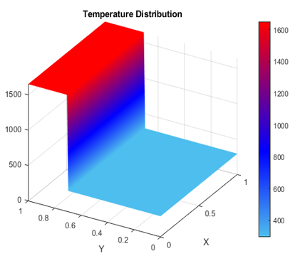
In Figure 2, temperature profile of the current composite is displayed evaluated by DIIM at 99 number of subintervals.
Figure 2. The thermal profile of composite of Problem 4.1 by DIIM at $n=99$
Example 2: In this example a composite with anisotropic materials is considered. In this example the coating is very thin and is of $0.1 \mathrm{~m}$ thickness. The top of the composite is at $1800^{\circ} \mathrm{K}$ and the bottom is at environmental temperature $295^{\circ} \mathrm{K}$. The thermal conductivity of the composite is uniform in $x$-direction by varies in both layers in y-directions causing discontinuity. Thermal conductivity of the composite is $1 \mathrm{~W}$ $\mathrm{Km}^{-1}$ in $x$-direction. In y-direction, it is $30^{\circ} \mathrm{W} \mathrm{Km}^{-1}$ of the substrate and $5^{\circ} \mathrm{W} \mathrm{Km}^{-1}$ of the coating. The main jumps along the interface are given as
$\begin{gathered}{[T]=1504} \\ {\left[\beta T_y\right]=-25}\end{gathered}$
For determining the temperature distribution in the current composite, DIIM is applied on steady state heat conduction equation incorporating the above jumps. The error in the solution is obtained using the exact solution
$T_e=\left\{\begin{array}{cc}y+295, & 0<y<0.9 \\ y+1799, & y>0.9\end{array}\right.$
The maximum absolute error at some grids is displayed in Table 3. It can be seen that the numerical solution achieved is highly accurate even at small number of subintervals.
The temperature variation along a cross section $x=0.5$ is demonstrated in Table 4 and compared with exact solution. It can be easily observed that the coating is not letting the temperature of the substrate increase even with the exposure of high heat. The last row in Table 4 belongs to the coating layer of the composite and rest of the points are in substrate layer. It can be clearly seen that at every point in both layers, the current approach provides great agreement with the exact solution.
Table 3. Maximum absolute error at arbitrary grids for Example 2
|
$\boldsymbol{n}$ |
$\left\|E_n\right\|_{\infty}$ |
|
11 |
$1.59 \times 10^{-12}$ |
|
12 |
$1.36 \times 10^{-12}$ |
|
21 |
$3.58 \times 10^{-12}$ |
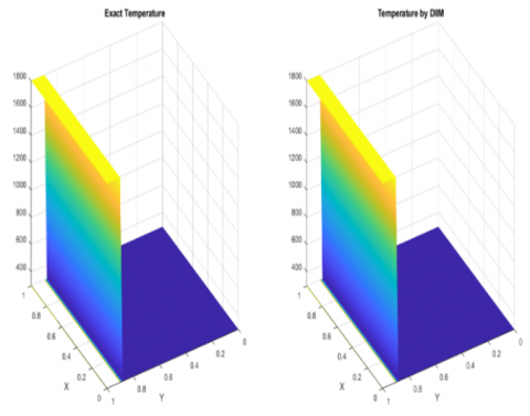
Figure 3 displays the comparative thermal profile of the composite under current boundary conditions by considering 50 subintervals. The left image in Figure 3 shows the exact thermal profile and the right one is obtained by current approach. It can be clearly observed that both profiles agree perfectly.
Figure 3. The comparison between exact and numerically obtained thermal profile of the composite in problem-2 at $n=50$
Problem 3: In this case the substrate is coated with 0.2 m thick layer of some FGM coating. The thermal conductivities of substrate and the coating is 20 W°Km-1 and 1oW Km-1 respectively. The jumps across the interface are given as
$\begin{gathered}{[T]=1701.28} \\ {\left[\beta \frac{\partial T}{\partial y}\right]=-42.28}\end{gathered}$
Table 4. Comparison of exact and numerically obtained temperature distribution at cross section $x=0.5$ at $n=24$ in problem 2
|
y |
Exact Temperature(oK) |
Temperature (oK)Obtained by DIIM |
|
0.15 |
295.15 |
295.1500000000000 |
|
0.25 |
295.25 |
295.2500000000002 |
|
0.35 |
295.35 |
295.3500000000004 |
|
0.45 |
295.45 |
295.4500000000004 |
|
0.55 |
295.55 |
295.5500000000004 |
|
0.65 |
295.65 |
295.6500000000003 |
|
0.75 |
295.75 |
295.7500000000001 |
|
0.85 |
295.85 |
295.8499999999992 |
|
0.95 |
1799.95 |
1799.949999999999 |
The error of the solution of steady state heat conduction equation of the current problem by decomposed immersed interface method is analyzed in Table 5 at different grid levels using the analytical solution of the problem.
$T_e=\left\{\begin{array}{c}e^y+294, \text { in } \Omega_1 \\ e^y-e+2000, \text { in } \Omega_2\end{array}\right.$
where, $\Omega_1$ denotes the region of the substrate and $\Omega_2$ denotes the region of the coating. The Table 5 indicates that the method is well suited, highly accurate for current problem.
Table 5. Maximum absolute error at arbitrary grids for Problem-3
|
$\boldsymbol{n}$ |
$\left\|E_n\right\|_{\infty}$ |
|
12 |
$6.46223315122825 \times 10^{-1}$ |
|
24 |
$1.422554756800309 \times 10^{-4}$ |
|
48 |
$1.130003477101127 \times 10^{-5}$ |
In Table 6 the exact temperature evaluated by analytical solution and the temperature obtained by the DIIM are compared at random 10 points at an arbitrary data $n=53$ at cross section $x=0.4716 \mathrm{~m}$ to demonstrate the efficiency of the current approach in evaluating the thermal profile of such composite.
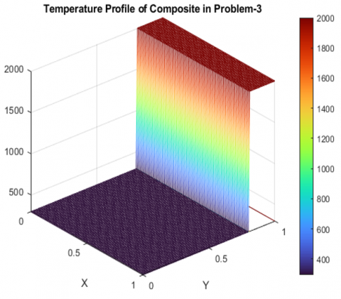
In Table 6 , the important of FGM coating can be observed. Even when the top is exposed to high heat $2000^{\circ} \mathrm{K}$, temperature of the substrate is maintained near $295^{\circ} \mathrm{K}$. The interface between two layers is at 0.8 and in the Table 6 , eighth and ninth entry is near the interface but the accuracy of the current approach is not disturbed. In Figure 4 the temperature distribution of the current composite is displayed at $n=99$.
Table 6. Comparison of exact and numerically obtained temperature distribution at cross section $x=0.5$ at $n=53$ in problem 3
|
y |
Exact Temperature (oK) |
Temperature (oK) Obtained by DIIM |
|
0.1132075 |
295.119864 |
295.119865 |
|
0.226415 |
295.254096 |
295.254096 |
|
0.339623 |
295.404418 |
295.404417 |
|
0.452830 |
295.572757 |
295.572755 |
|
0.528302 |
295.696050 |
295.696047 |
|
0.679245 |
295.972389 |
295.972383 |
|
0.754717 |
296.127009 |
296.127001 |
|
0.849057 |
1999.619159 |
1999.619152 |
|
0.924528 |
1999.802397 |
1999.802394 |
|
0.981132 |
1999.949192 |
1999.949192 |
Figure 4. Temperature profile of the composite in Problem-3 at 99 number of subintervals
In this work, thermal analysis is done of a FGM coated composite in which the bottom layer is of some homogeneous substrate and the top layer is a coating of some functionally graded material (FGM). The composite is exposed to high heat at the top and the purpose of the study is whether the FGM coating is helpful in maintaining the temperature of the substrate even with high heat exposure at one end. The challenge is that the contact between the two layers in the composite is not perfect so many standard methods are not successful in this case. Decomposed immersed interface method (DIIM) is applied to solve the steady state heat conduction equation for finding the temperature distribution in the current study as it incorporates various types of jumps in the standard finite difference scheme and is highly accurate and efficient. The current study demonstrates that the FGM coating effectively maintains the substrate temperature and shields it from physical damage caused by high heat. This approach has high scope in thermal analysis of many other composite systems for example composite fin, mixed material multilayered composites, composite beams, reinforced materials, composite pipes etc.
[1] Brindley, W.J. (1995). Properties of plasma sprayed bond coats, Proceedings of Thermal Barrier Coating Workshop.NASA-Lewis. https://ntrs.nasa.gov/api/citations/19950019699/downloads/19950019699.pdf.
[2] DeMasi-Marcin, J.T., Gupta, D.K. (1994). Protective coatings in the gas turbine engine. Surface and Coatings Technology, 68-69. https://www.sciencedirect.com/science/article/abs/pii/0257897294901295.
[3] Sheffter, K.D., Gupta, D.K. (1988). Current Status and Future Trends in Turbine Application of Thermal Barrier Coatings. Journal of Engineering for Gas Turbine and Power. Transactions of ASME, 110: 605-609. https://doi.org/10.1115/1.3240178
[4] Low, I.M. (2006). Ceramic-Matrix Composites. Woodhead Publishing, 1-6. https://doi.org/10.1115/1.3240178
[5] Joshi, P., Kumar, M. (2012). Mathematical model and computer simulation of three-dimensional thin film elliptic interface problems. Computers & Mathematics with Applications, 63(1): 25-35. https://doi.org/10.1016/j.camwa.2011.10.054
[6] Kumar, M., Joshi, P. (2012). A mathematical model and numerical solution of a one-dimensional steady state heat conduction problem by using high order immersed interface method on non-uniform mesh. International Journal of Nonlinear Science (IJNS), 14(1): 11-22.
[7] Kumar, M., Joshi, P. (2013). Mathematical modelling and computer simulation of steady state heat conduction in anisotropic multi-layered bodies. International Journal of Computing Science and Mathematics, 4(2): 85-119. https://doi.org/10.1504/IJCSM.2013.055195
[8] Joshi, P., Kumar, M. (2014). Mathematical modelling and numerical simulation of temperature distribution in inhomogeneous composite systems with imperfect interface. Engineering Structures and Technologies, 6(2): 77-85. https://doi.org/10.3846/2029882X.2014.972643
[9] Kumar, M., Joshi, P. (2012). Some numerical techniques to solve elliptic interface problems. Numerical Methods for Partial Differential Equations, 28(1): 94-114. https://doi.org/10.1002/num.20609
[10] Pathak, M., Joshi, P. (2021). Thermal analysis of some fin problems using improved iteration method. International Journal of Applied and Computational Mathematics, 7: 49. https://doi.org/10.1007/s40819-021-00964-0
[11] Maheshwar, P., Joshi, P., Nisar, K.S. (2022). Numerical investigation of fluid flow and heat transfer in micropolar fluids over a stretching domain. Journal of Thermal Analysis and Calorimetry, 147: 10637-10646. https://doi.org/10.1007/s10973-022-11268-w
[12] Pathak, M., Joshi, P. (2015). A high order solution of three-dimensional time dependent nonlinear convective - diffusive problem using modified variational iteration method. International Journal of Science and Engineering, 8(1):1-5. https://doi.org/10.12777/ijse.8.1.1-5
[13] Lee, Y.D., Erdogan, F. (1998). Interface cracking of FGM coatings under steady-state heat flow. Engineering Fracture Mechanics, 59(3): 361-380. https://doi.org/10.1016/S0013-7944(97)00137-9
[14] Perkowski, D.M. (2014). On axisymmetric heat conduction problem for FGM layeron homogeneous substrate. International Communications in Heat and Mass Transfer, 57: 157-162. https://doi.org/10.1016/j.icheatmasstransfer.2014.07.021
[15] Berthelsen, P.A. (2004). A decomposed immersed interface method for variable coefficient elliptic equations with non-smooth and discontinuous solutions. Journal of Computational Physics, 197(1): 364-386. https://doi.org/10.1016/j.jcp.2003.12.003
[16] Alaa, S., Irwansyah, Kurniawidi, D.W., Rahayu, S. (2020). The analytical and numerical solutions of two dimensional heat transfer equation in a multilayered composite cylinder. IOP Conference Series: Materials Science and Engineering, 858(1): 012038. https://doi.org/10.1088/1757-899X/858/1/012038
[17] Aljehania, A., Nitsche, L., Al-Hallaj, S. (2020). Numerical modeling of transient heat transfer in a phase change composite thermal energy storage (PCC-TES) system for air conditioning applications. Applied Thermal Engineering, 164: 114522. https://doi.org/10.1016/j.applthermaleng.2019.114522
[18] Skerget, L., Tadeu, A., Antonio, J. (2020). Numerical simulation of heat transport in multilayered composite pipe. Engineering Analysis with Boundary Elements, 120: 28-37. https://doi.org/10.1016/j.enganabound.2020.07.027
[19] Wang, L.H., Zhang, R., Guo, R. Liu, G.Y. (2024). Finite element method with 3D polyhedron-octree for the analysis of heat conduction and thermal stresses in composite materials. Composite Structures, 327: 117649. https://doi.org/10.1016/j.compstruct.2023.117649
[20] Ibouroi, L.A., Vidal, P., Gallimard, L., Ranc, I. (2022). Thermal analysis of composite beam structure based on a variable separation method for any volume heat source locations and temporal variations. Composite Structures, 300: 116154. https://doi.org/10.1016/j.compstruct.2022.116154
[21] Zhai, F.M., Cao, L.Q. (2021). A multiscale parallel algorithm for dual-phase-lagging heat conduction equation in composite materials. Journal of Computational and Applied Mathematics, 381: 113024. https://doi.org/10.1016/j.cam.2020.11302