Amara Fethallah | Samir Deghboudj*
© 2022 IIETA. This article is published by IIETA and is licensed under the CC BY 4.0 license (http://creativecommons.org/licenses/by/4.0/).
OPEN ACCESS
In many engineering fields such as aerospace, marine, automotive and mechanical, the design of planar structures consisting of rectangular plates commonly requires the use of holes as a technological solution in fastening assemblies. The major goal of this research is to examine the impact of stress concentration factors (SCF) in the specific case of planar structures, highlight their relevance as a potential source of structural failure, and compare the various techniques employed to gauge their magnitude. Particular emphasis will be placed on rectangular plates with holes since these plates' shape discontinuities alter the stress field, leading to a local increase in the stress field that, if not accurately predicted and analyzed at the design stage, could endanger the entire structure. For the studied case (rectangular plate with central hole subjected to uniform tensile field), a new finite element formulation based on 3-noded triangular element has been suggested to estimate the field variables (stress). MATLAB programming has been developed by considering this element. Analysis has been carried out for the same structure (rectangular plate) with analysis software Abaqus. Finding was compared to several analytical solutions published in the literature, based on Heywood, Howland, and Flynn formulations. Obtained results were in good agreement.
stress concentration factor, plate with hole finite element method, MATLAB programming
The phenomena of stress concentration around geometric singularities that arise in structures and devices is extremely important. It is the main cause of crack propagation and failure [1]. The stress concentration area is often the site of initiation of fatigue cracks but can also be the origin of a sudden break in the case of a brittle material. The stress concentration near a geometric discontinuity, such as a hole, is predicted by a characteristic that is commonly referred to as the stress concentration factor (SCF) [1]. In the case of a perforated plate, this parameter called Kt is defined as the ratio of the maximal real stress σmax acting around the hole to the nominal stress σnom imposed at the plate border [2]. In 1898, Kirsh was the first to emphasize the phenomenon of stress concentration [3]. It was for a problem of measuring the stresses around a hole. Afterward, analytical solutions were progressively found and proposed, by different authors for structures with increasingly complex geometries. Several analytical and numerical types of researches have been carried out on the stress concentration phenomena. Among the early works, we can quote the famous contributions of Heywood [4], Howland [5], Pilkey [6], and Peterson [7]. Heywood, Peterson, and Pilkey have studied a variety of isotropic structures with several different kinds of holes. Howland found the answer to the problem posed by a rectangular plate with a hole in the center that is being loaded tensile. Timoshenko and Goodier (1951), have carried out a survey on stress concentration phenomena surrounding holes in the case of infinite width plates based on a classical approach employing a two-dimensional solution [8]. In an interesting work [9], Jain and Mittal studied the influence of hole diameter concerning plate width upon stress concentration factor and strain in isotropic, orthotropic, and laminated composite plates, under various transverse static loading conditions. Giare and Shabahang [10] developed a novel procedure to mitigate the stress concentration around the hole in an isotropic plate using composite patches. Zappalorto and Carraro proposed an engineering formula to estimate the stress concentration factor for orthotropic composite plates [11]. The study conducted by Jafari and Ardalani [12] involves the stress distribution surrounding regular holes infinite metal plates, under the assumption of a plane stress state and a uniaxial loading condition. The authors proposed an analytical solution based on Muskhelishvili complex variables. Nowadays, computational techniques and especially the finite element method are widely used to analyze the stress concentration phenomena for different configurations of structures with cutouts. The use of adapted software based on this method and featuring new techniques such as automatic generation of meshes and their refinement has considerably improved the accuracy of calculations. Khechai et al. [13] investigated the stress concentration phenomena in isotropic and laminated plates with inclined elliptical holes using a numerical model. They introduced a finite element analysis using two finite elements in conjunction. A linear isoparametric membrane element was the first finite element, and a high precision Hermitian element was the second. In Ref [14] the authors curried out an interesting experimental, analytical, and finite element study of stress concentration factors for both isotropic and composite materials.
In spite of the enormous technological progress in the field of structural assembly, the joining by screwing and riveting requiring the use of holes, remains unavoidable especially in the fields of aeronautics, space, naval and automotive industry. Although a great deal of research has been dedicated to the phenomenon of stress concentration in planar structures with holes, under different solicitations, it presents many complexities and gaps.
This study is intended as a contribution to this work. Its main objective is to investigate the stress field at the edge of the hole of a rectangular plate loaded in tension and to analyze the stress concentration phenomena in case of steel rectangular isotropic plates with central circular hole. The application of the finite element approach is necessary and becomes essential in order to appropriately identify the resulting stress field and subsequently the stress concentration parameters. A finite element of the three-node triangular constant strain element has been presented in this paper. MATLAB programming has been developed by considering this element. The stress field could be precisely determined in the edge of the hole. The obtained results were confirmed with other results provided by the ABAQUS software. The agreement of the findings was outstanding. The second part of this work evaluates the global and the net stress concentration factor (SCF) by suggested element and Abaqus software, comparing them with some commonly used analytical methods. As well, the results are in good agreement.
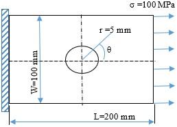
The fundamental purpose of studying thin plates under mechanical loadings, such as pressures and uniformly distributed forces, is to identify the effect on the structural response to the loads [15]. The objective of this research is to investigate the distribution of stress field and stress concentration factor, in isotropic plates subjected to tension load around a circular central hole. Consider a rectangular isotropic thin plate with a circular central hole of diameter (d) and thickness (t), subjected to pure tensile stress in the direction of the plate's axis x (Figure 1); the plate's dimensions are assumed to be sufficiently large in comparison to the radius r, and volume forces are ignored in-plane stress. According to literature the analytical solution of the plane elasticity distribution of the stress field in polar coordinates (r, θ) [16-19]:
$\sigma_{ rr }=\frac{\sigma}{2}\left[1-\frac{ a ^2}{ r ^2}+\left(1+3 \frac{ a ^4}{ r ^4}-4 \frac{ a ^2}{ r ^2}\right) \cdot \cos 2 \theta\right]$
$\sigma_{\theta \theta}=\frac{\sigma}{2}\left[1+\frac{ a ^2}{ r ^2}-\left(1+3 \frac{ a ^4}{ r ^4}\right) \cdot \cos 2 \theta\right]$
$\sigma_{ r \theta}=-\frac{\sigma}{2}\left(1-3 \frac{ a ^4}{ r ^4}+2 \frac{ a ^2}{ r ^2}\right). \sin 2 \theta$ (1)
The following transformation is used to find the relationship between stresses stated in polar coordinates (r,θ) and those expressed in the Cartesian coordinate system (x,y):
$[\sigma]_{( x , y )}=[ T ]^{ t }[\sigma]_{( r , \theta )}[ T ]$ (2)
Figure 1. Plate with central hole under uniaxial tension field
In Eq. (2) [T] represents the passage matrix:
$T =\left[\begin{array}{ccc}\cos \theta & \sin \theta & 0 \\ -\sin \theta & \cos \theta & 0 \\ 0 & 0 & 1\end{array}\right]$ (3)
This leads to the expression of the stress tensor expressed in the Cartesian coordinate system:
$\sigma_{ xx }=\sigma_{ rr } \cos ^2 \theta+\sigma_{\theta \theta} \sin ^2 \theta-\sigma_{ r \theta} \sin 2 \theta$
$\sigma_{ yy }=\sigma_{ rr } \sin ^2 \theta+\sigma_{\theta \theta} \cos ^2 \theta+\sigma_{ r \theta} \sin 2 \theta$
$\sigma_{ xy }=\frac{\sigma_{ rr }-\sigma_{\theta \theta}}{2} \sin 2 \theta+\sigma_{ r \theta} \cos 2 \theta$ (4)
The SCF is defined, as the ratio of the maximum stress, σmax, recorded on the plate by the nominal stress, σnom, calculated in the hole section, according to Eq. (5).
$K _{ t }=\frac{\sigma_{\max }}{\sigma_{ nom }}$ (5)
where, σmax is evaluated by numerical methods or by analytical approaches in the case of simple geometries. It is also estimated by experimental methods such as photoelasticity and digital image correlation. On the other hand, σnom can be evaluated using strength material formulas. Several formulas based on experimental data fitting are used to calculate the SCF. The author in reference [20] proposed Eq. (6) as potential expression for determining SCF in case of isotropic plate with central hole.
$K _{ t }=3-3.13\left(\frac{ d }{ W }\right)+3.66\left(\frac{ d }{ W }\right)^2-1.53\left(\frac{ d }{ W }\right)^3$ (6)
According to Heywood investigation [4], in case of finite rectangular isotropic plate with a central hole subjected to a unidirectional axial force, the SCF is given by the following equation:
$\frac{3}{ K _{ t }}=\frac{3\left(1-\frac{ d }{ W }\right)}{2+3\left(1-\frac{ d }{ W }\right)^3}$ (7)
Howland [5] provided the following formula for the global stress concentration factor Kt for an isotropic rectangular plate with a central circular hole under tensile stress:
$K _{ t }=0.284+\frac{2}{\left(1-\frac{ d }{ W }\right)}-0.6\left(1-\frac{ d }{ W }\right)+1.32\left(1-\frac{ d }{ W }\right)^2$ (8)
Another manner of calculating the stress concentration factor is to use the average stress over the net section taking into account the hole. The stress concentration factor in this setting is referred to as the net stress concentration factor Kn, and it can be related to the global stress concentration factor Kt by using the subsequent formula [1, 5, 21]:
$K _{ n }= K _{ t }\left(1-\frac{ d }{ W }\right)$ (9)
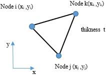
In this work, an isotropic three-node triangular constant strain element (CSE) was used. As shown in Figure 2, the proposed element is defined by one node at each corner. In the global Cartesian coordinate system, the nodes have coordinates (xi, yi), (xj, yj), and (xk, yk). Each node provides two degrees of freedom, u and v, which represent translation in both the global x and y directions. In the case of plane stress, the stress-strain relationship is given as follow:
$\{\sigma\}=[ D ]\{\varepsilon\}$ (10)
where, [D] is the matrix form of the Hooke’s law in a two-dimensional space, {σ} and {ε} are stress and strain tensors, respectively. Explicitly:
$\left(\begin{array}{c}\sigma_{ xx } \\ \sigma_{ yy } \\ \tau_{ xy }\end{array}\right)=\left(\frac{ E }{1-v^2}\right)\left[\begin{array}{ccc}1 & v & 0 \\ v & 1 & 0 \\ 0 & 0 & \frac{(1-v)}{2}\end{array}\right]\left(\begin{array}{c}\varepsilon_{ xx } \\ \varepsilon_{ yy } \\ \gamma_{ xy }\end{array}\right)$ (11)
$\sigma_{ xx }, \sigma_{ yy }$, are the components of normal stresses and $\tau_{ xy }$ the component of shear stress over x-y plane. For this three-node element, the shape functions are given as:
$N _{ i }( x , y )=\frac{\alpha_{ i }+\beta_{ i }+\lambda_{ i }}{ A }$
$N _{ j }( x , y )=\frac{\alpha_{ j }+\beta_{ j }+\lambda_{ j }}{ A }$
$N _{ k }( x , y )=\frac{\alpha_{ k }+\beta_{ k }+\lambda_{ k }}{ A }$ (12)
where,
$\begin{array}{cccc} & A =\left|\begin{array}{ccc}1 & x _{ i } & y _{ i } \\ 1 & x _{ j } & y _{ j } \\ 1 & x _{ k } & y _{ k }\end{array}\right| & \\ \alpha_{ i }= x _{ j } y _{ k }- x _{ k } y _{ j } & \alpha_{ j }= x _{ k } y _{ i }- x _{ i } y _{ k } & \alpha_{ k }= x _{ i } y _{ j }- x _{ j } y _{ i } \\ \beta_{ i }= y _{ j }- y _{ k } & \beta_{ j }= y _{ k }- y _{ i } & \beta_{ k }= y _{ i }- y _{ j } \\ \lambda_{ i }= x _{ k }- x _{ j } & \lambda_{ j }= x _{ i }- x _{ k } & \lambda_{ k }= x _{ j }- x _{ i }\end{array}$ (13)
The displacement field over the element is approximated in a matrix form as:
$\left\{\begin{array}{l}u \\ v\end{array}\right\}=\left[\begin{array}{cccccc}N_i & 0 & N_j & 0 & N_k & 0 \\ 0 & N_i & 0 & N_j & 0 & N_k\end{array}\right]\left\{\begin{array}{c}u_i \\ v_i \\ u_j \\ v_j \\ u_k \\ v_k\end{array}\right\}$ (14)
Knowing that:
$\left(\begin{array}{c}\varepsilon_{ x } \\ \varepsilon_{ y } \\ \gamma_{ xy }\end{array}\right)=\left(\begin{array}{c}\frac{\partial u }{\partial x } \\ \frac{\partial v }{\partial y } \\ \frac{\partial u }{\partial x }+\frac{\partial v }{\partial y }\end{array}\right)$ (15)
The plane-strain can be derived from Eq. (5) as:
$\left(\begin{array}{c}\varepsilon_{ x } \\ \varepsilon_{ y } \\ \gamma_{ xy }\end{array}\right)=\left[\begin{array}{cccccc}\frac{\partial N _{ i }}{\partial x } & 0 & \frac{\partial N _{ j }}{\partial x } & 0 & \frac{\partial N _{ k }}{\partial x } & 0 \\ 0 & \frac{\partial N _{ j }}{\partial y } & 0 & \frac{\partial N _{ j }}{\partial y } & 0 & \frac{\partial N _{ k }}{\partial y } \\ \frac{\partial N _{ i }}{\partial y } & \frac{\partial N _{ i }}{\partial x } & \frac{\partial N_j }{\partial y } & \frac{\partial N _{ j }}{\partial x } & \frac{\partial N_k }{\partial x } & \frac{\partial N _{ k }}{\partial y }\end{array}\right]\left(\begin{array}{c} u _{ i } \\ v _{ i } \\ u _{ j } \\ v _{ j } \\ u _{ k } \\ v _{ k }\end{array}\right)$ (16)
These relations can be written in a matrix form as:
$\{\varepsilon\}=[ L ]\{ U \}$ (17)
where, [L] is a linear differential operator. Substituting Eq. (14) and using (12) into Eq. (16) yields
$\{\varepsilon\}=[ B ]\{ U \}$ (18)
Knowing that total strain energy of the element is defined as:
$A=\int_V \frac{1}{2}[\varepsilon]^{ T }[ D ][\varepsilon] dV$ (19)
Eq. (20) is obtained by replacing Eq. (18) into Eq. (19):
$\Lambda=\frac{1}{2} \int_V(U)^{ T }[ B ]^{ T }[ D ][ B ]( U ) dV$ (20)
$[ B ]=\frac{1}{2 A }\left[\begin{array}{cccccc}\beta_{ i } & 0 & \beta_{ j } & 0 & \beta_{ k } & 0 \\ 0 & \lambda_{ i } & 0 & \lambda_{ j } & 0 & \lambda_{ k } \\ \lambda_{ i } & \beta_{ i } & \lambda_{ j } & \beta_{ j } & \lambda_{ k } & \beta_{ k }\end{array}\right]$ (21)
In Eq. (21), [B] stands for the strain-displacement matrix, $(\beta i , \beta j , \beta k , \lambda i , \lambda j , \lambda k )$ represents the coefficients stated in Eq. (12), and A indicates the triangle element's area. Based on the principle of minimum potential energy, the first variation provides the expression of the elementary stiffness matrix and the vector loads as:
$\frac{\partial A}{\partial U}=(A \cdot t)[B]^T[D][B]( U )=\{F\}$ (22)
With:
$[ K ]^{ e }=[ B ]^{ T }[ D ][ B ] t . A$ (23)
Figure 2. Three-node triangular constant strain element
The stiffness matrix of the assembly is constructed after the element stiffness matrices and element vectors have been calculated in the global coordinate system. The nodal variables are generalized displacements, which can be translations, rotations, or other spatial derivatives of them. Let's denote the total number of elements and the nodal degree of freedom 'nelem' and 'sdof,' respectively. sdof x sdof is the order of the constructed stiffness matrix [K], and P is the typical load vector of dimension sdof x1. Thus, the global stiffness matrix and the global load vector can be obtained by the following algebraic sum:
$[K]=\sum_{e=1}^{n e l e m}[K]^e$ (24)
And:
$[ F ]=\sum_{ e =1}^{\text {nelem }}\{ f \}^{\text {e }}$ (25)
This analysis was performed for a steel isotropic rectangular plate of length L=200 mm, width W=100 and thickness of 1 mm, with a central hole of radius r=5 mm. The plate has elastic modulus E = 210 000 MPa, Poisson’s ratio υ = 0.33 and mass density $\rho$= 7800 kg/m3. One of the plate's ends is fixed, while the other is subjected to a unidirectional tensile load of 100 MPa, as indicated in Figure 1. Only one quarter of the plate was considered to compute the stress concentration factor due to geometric and material symmetry. The x-axis points are constrained in the y direction, whereas the y-axis points are constrained in the x direction. When an axial force is applied to the plate, it creates a complex stress distribution not only in the localized region of the hole edge, but also in the surrounding zones. To accurately determine the resulting stress field and subsequently the stress concentration factors, the use of the finite element method is required and becomes indispensable. In this work we will provide a finite element of type three-node triangular constant strain element. The plate is descritized in several elements as presented and detailed in Section 5. A convergence study of the meshing has been conducted. The validation of the proposed element has been made through the confrontation of the results obtained with others provided by the computational code ABAQUS after the achievement of the simulation of the same problem with the identical conditions of geometry and mechanical characteristics of the plate object of this research. Global and net stress concentration factors, Kt and Kn, respectively, were computed for varying ratios (d/W) in range of 0.1 to 0.6, using several analytical approaches including Heywood, Howland, and Flynn formulations (Eqns. (6), (7), and (8)), and then they were being compared with the solutions obtained by suggested triangular element and ABAQUS software. The resulting values of Kt and Kn are summarized in Table 2.
5.1 Validation of the proposed finite element
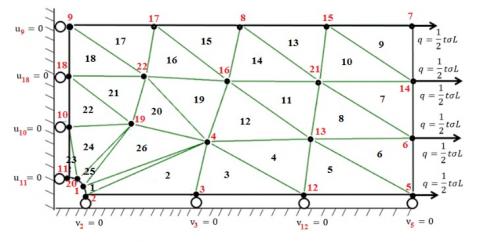
To carry out the finite element analysis of the plate, we firstly used 26 elements to discretize the domain as shown in Figure 3. Notice that the nodes coordinates were generated using Abaqus Mesh module. The coordinates x and y of the nodes are given in the form of a matrix of dimension (nnd, 2). The element connectivity is given in the matrix connec(nel, 3). A load of 100 MPa is applied at nodes numbered 7, 6, 14 and 5. The force was assembled into the global force vector in the main program. To read the data, we used a M-file. The input data for this case consist of:
nnd=22; number of nodes
nel=26; number of elements
nne=3; number of nodes per element
nodof=2; number of degrees of freedom per node
Figure 3. Finite element discretization with 26 linear triangular elements
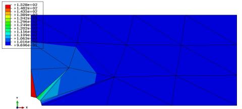
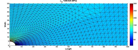
ABAQUS finite element analysis software is renowned for its reliability and efficiency. It is indeed a capable way of analyzing a wide range of problems. Elasticity, fluid motion, heat transport and ectromagnetism are among the challenges that this software can address. In addition, it can also offer the best solutions to linear, nonlinear, explicit and dynamic problems. In this study numerical simulation analysis was carried out using ABAQUS software code to approve the suggested finite element results. A static general step was used to determine the stresses. One quarter of the plate is discretized into a finite number of rectangular elements. The CPS3 3-node linear plane stress element was employed as depicted in Figure 4b and Figure 5b. The stress field surrounding the hole is provided by the computational program. It also gives the maximum stresses values, allowing the stress concentration factor (SCF) to be calculated using Eq. (5). The results are first displayed as they were provided by the calculation program performed with a coarse mesh. Figure 4(a) and Figure 5(a) show the iso-values of the stress field given by the calculation program. To validate the proposed finite element, a simulation under Abaqus software was performed with the same meshing density. Figure 4(b) and Figure 5(b) present the same profile given by Abaqus. Furthermore, because the stress field near the hole changes rapidly, a higher mesh density with smaller elements is used towards the hole boundary. Nevertheless, it is very useful to carry out a convergence study of the mesh. We have chosen several mesh densities. Convergence was achieved with a mesh size of 1442 elements. The relative errors were calculated using the following equation:
$e(\%)=\left|\frac{ { FEM }- { Theoritical } \quad}{\text { FEM }}\right| \times 100 \%$ (26)
(a)
(b)
Figure 4. Iso-stress values, in case of one quarter of thea plate modeled using 26 elements: a) the calculation program; b) Abaqus simulation
Table 1. Numerical results obtained from the convergence study
|
Stress Concentration Factor (SCF) |
||||
|
Elements |
Theoretical |
Present |
Abaqus |
Error (%) |
|
10 |
3.000 |
1.333 |
1.333 |
125.056 |
|
14 |
3.000 |
1.341 |
1.341 |
123.7147 |
|
26 |
3.000 |
1.528 |
1.528 |
96.335 |
|
48 |
3.000 |
1.73 |
1.73 |
73.410 |
|
68 |
3.000 |
1.843 |
1.843 |
62.778 |
|
104 |
3.000 |
1.979 |
1.979 |
51.593 |
|
130 |
3.000 |
2.091 |
2.091 |
43.472 |
|
272 |
3.000 |
2.37 |
2.37 |
26.582 |
|
384 |
3.000 |
2.52 |
2.52 |
19.047 |
|
436 |
3.000 |
2.561 |
2.561 |
17.141 |
|
578 |
3.000 |
2.662 |
2.662 |
12.697 |
|
672 |
3.000 |
2.706 |
2.706 |
10.865 |
|
740 |
3.000 |
2.747 |
2.747 |
9.210 |
|
846 |
3.000 |
2.783 |
2.783 |
7.797 |
|
922 |
3.000 |
2.817 |
2.817 |
6.496 |
|
1040 |
3.000 |
2.847 |
2.847 |
5.374 |
|
1442 |
3.000 |
2.996 |
2.996 |
0.133 |
The numerical results obtained from the convergence study are depicted in Figure 6 and Table 1. From Figure 6, one can see clearly the convergence obtained for the proposed finite element.
(a)
(b)
Figure 5. Iso-stress values, in case of one quarter of the plate modeled using 1442 elements: a) the calculation program; b) Abaqus simulation
Figure 6. Convergence study
5.2 Stress concentration analysis
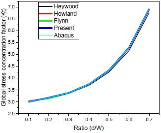
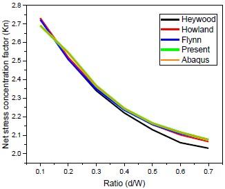
Numerical analysis was conducted using the FEM ABAQUS package [22] and the proposed finite element to validate the analytical findings. Figure 4 and Figure 5 illustrate the FEM models that were used. The finite element mesh is refined around the holes in both numerical cases. A linear elastic approach is employed to model the material behavior. For various (d/W) ratios in range of 0.1 to 0.6, global and net stress concentration factors for the isotropic plates with central hole were calculated, using Heywood, Howland and Flynn formulations (Eqns. (6), (7), and (8)), in order to be compared with FE results. For numerical methods, in each computation step, global and net stress concentration factors are obtained by dividing maximum stress concentration extracted from MATLAB programming and Abaqus software, by the nominal and average stress according to Eq. (5) and Eq. (9). Figure 7, Figure 8 and Tables 2 present the main numerical results. Three analytical techniques, as well as FEM procedures, were used to compare the stresses. Maximum and stress distribution around the hole with d/W = 0.1 are shown in Figure 4. As the (d/W) ratio rises, the global stress concentration factor Kt values rise. For a growth in diameter, this suggests a rise in the stress concentration factor. The net stress concentration factor Kn, on the other hand, decreases when the (d/W) ratio increases, indicating a decrease in SCF for an increase in diameter. We can also notice that for the case of the global stress concentration factor Kt, the findings obtained by the suggested finite element are quite similar with the results of the theoretical approaches used, as shown in Figure 7 and Table 2. As depicted in Figure 8, when comparing the results provides by the proposed element to those generated by the analytical approaches, a substantial difference is noticed for the net stress concentration factor Kn when the ratio (d/W) is greater than 0.4. This can be explained by the fact that plastic deformation occurs along the hole edge of a steel plate with bigger hole diameters (a/w greater than 0.4). However, the present FE analysis was performed in the context of the elastic analysis. Tables 1 and 2 show that the values of the stress concentration factor, global Kt, and net Kn generated by the MATLAB program based on the present element and those provided by Abaqus are in perfect accord.
Table 2. Variation of the global and net SCF with respect to (d/W) ratio, using the proposed finite element and commonly used analytical approaches
|
|
Heywood (Eq.) |
Howland (Eq.) |
Flynn (Eq.) |
FEM present |
FEM Abaqus |
|||||
|
d/W |
Kt |
Kn |
Kt |
Kn |
Kt |
Kn |
Kt |
Kn |
Kt |
Kn |
|
0.1 |
3.03 |
2.73 |
3.035 |
2.731 |
3.024 |
2.722 |
2.99 |
2.691 |
2.99 |
2.691 |
|
0.2 |
3.14 |
2.51 |
3.148 |
2.519 |
3.135 |
2.508 |
3.18 |
2.544 |
3.18 |
2.544 |
|
0.3 |
3.35 |
2.34 |
3.367 |
2.357 |
3.355 |
2.349 |
3.38 |
2.366 |
3.38 |
2.366 |
|
0.4 |
3.69 |
2.22 |
3.732 |
2.239 |
3.726 |
2.235 |
3.74 |
2.244 |
3.74 |
2.244 |
|
0.5 |
4.25 |
2.13 |
4.314 |
2.157 |
4.317 |
2.158 |
4.33 |
2.165 |
4.33 |
2.165 |
|
0.6 |
5.16 |
2.06 |
5.255 |
2.102 |
5.272 |
2.109 |
5.29 |
2.116 |
5.29 |
2.116 |
|
0.7 |
6.76 |
2.03 |
6.889 |
2.066 |
6.925 |
2.077 |
6.92 |
2.076 |
6.92 |
2.076 |
Figure 8. Evolution of the net stress concentration factor Kn, with respect to (W/d) ratio
In this research, a triangular three-node constant strain element was suggested to compute the stress concentration factor (SCF) for a thin rectangular steel plate subjected to a tensile field. A comparison between the values of the global stress concentration coefficients (Kt) and net (Kn) generated by a MATLAB computational program based on the proposed finite element, by a simulation under Abaqus software and by commonly used analytical solutions has been carried out. The following findings can be inferred:
The authors like to thank the Algerian general direction of research (DGRSDT) for their support.
[1] Deghboudj, S., Satha, H., Boukhedena, W. (2016). Effect of shape factor upon stress concentration factor in isotropic/orthotropic plates with central hole subjected to tension load. U.P.B. Scientific Bulletin Series D, 78(4): 689-699.
[2] Deghboudj, S., Boukhedena, W, Satha, H. (2016). Numerical analysis of the stress concentration in a composite plate with two holes in a tensile field. Revue des Composites et des Matériaux Avancés, 26(2): 147-163. https://doi.org/10.3166/RCMA.26.147-163
[3] Rice, J. (1993). Mechanics of Solids. Encyclopedia Britannica.
[4] Heywood, R.B. (1952). Designing by Photoelasticity. Chapman & Hall.
[5] Howland, R.C.J. (1930). On the stresses in the neighborhood of a circular hole in a strip under tension. Philosophical Transactions of the Royal Society of London. Series A, 229(670-680): 49-86. https://doi.org/10.1098/RSTA.1930.0002
[6] Pilkey, W., Pilkey, D. (2008). Peterson's Stress Concentration Factors. John Wiley and Sons.
[7] Peterson, R. (2008). Stress Concentration Factors/RE Peterson. New York: Wiley.
[8] Timoshenko, S., Goodier, J. (1951). Theory of Elasticity. McGraw-Hill Book Company, Inc. New York.
[9] Jain, N., Mittal, N. (2008). Finite element analysis for stress concentration and deflection in isotropic, orthotropic and laminated composite plates with central circular hole under transverse static loading. Materials Science and Engineering: A, 498(1-2): 115-124. https://doi.org/10.1016/j.msea.2008.04.078
[10] Giare, G.S., Shabahang, R. (1989). The reduction of stress concentration around the hole in an isotropic plate using composite materials. Engineering fracture mechanics, 32(5): 757-766. https://doi.org/10.1016/0013-7944(89)90172-0
[11] Zappalorto, M., Carraro, P.A. (2015). An engineering formula for the stress concentration factor of orthotropic composite plates. Composites Part B: Engineering, 68: 51-58. https://doi.org/10.1016/j.compositesb.2014.08.020
[12] Jafari, M., Ardalani, E. (2016). Stress concentration in finite metallic plates with regular holes. International Journal of Mechanical Sciences, 106: 220-230. https://doi.org/10.1016/j.ijmecsci.2015.12.022
[13] Khechai, A., Tati, A., Belarbi, M.O., Guettala, A. (2019). Numerical analysis of stress concentration in isotropic and laminated plates with inclined elliptical holes. Journal of the Institution of Engineers (India): Series C, 100(3): 511-522. https://doi.org/10.1007/s40032-018-0448-4
[14] Mohamed Makki, M., Chokri, B. (2017). Experimental, analytical, and finite element study. Journal of Composite Materials, 51(11): 1583-1594. https://doi.org/10.1177/0021998316659915
[15] Diany, M. (2013). Effects of the position and the stress concentration factor. International Journal of Engineering Research & Technology, 2(12): 2278-0181. https://doi.org/10.17577/IJERTV2IS120103
[16] Jiang, Z., Zhang, R., Gong, S., Hou, J., Jin, X. (2021). An analytical method for plane elasticity problems involving circular boundaries. Journal of Physics: Conference Series, Volume 2002, 7th International Conference on Machinery, Material Science and Engineering Application (MMSE) 2021 24-25 July 2021, Hangzhou Radisson Hotel Platinum, Hangzhou, China.
[17] Kozera, I., Konopińska-Zmysłowska, V., Kujawa, M. (2019). Stress analysis of a strip under tension with a circular hole. In AIP Conference Proceedings, 2077(1): 020028. https://doi.org/10.1063/1.5091889
[18] Kasayapanand, N. (2008). Exact solution of double filled hole of an infinite plate. Journal of Mechanics of Materials and Structures, 3(2): 365-373.
[19] Boubeker, R., Hecini, M. (2017). Study of the mechanical behavior of orthotropic plates with a centered elliptic hole. Revue des Composites et des Materiaux Avances, 27(4): 381-398. https://doi.org/10.3166/rcma.2017.00020
[20] Flynn, P. (1969). Photoelastic comparison of stress concentrations due to semicircular grooves and a circular hole in a Tension Bar. Journal of Applied Mechanics, 36(4): 892-893. https://doi.org/10.1115/1.3564796
[21] Bakhshandeh, K., Rajabi, I., Rahimi, F. (2008). Investigation of stress concentration factor for finite-width orthotropic rectangular plates with a circular opening using three-dimensional finite element model. Strojniski Vestnik - Journal of Mechanical Engineering, 54(2): 140-147.
[22] ABAQUS/Standard User's Manual, Version 6.14. http://130.149.89.49:2080/v6.14/pdf_books/CAE.pdf.