Mohammad Hossein Ahmadi* | Mahyar Ghazvini | Alireza Baghban | Masoud Hadipoor | Parinaz Seifaddini | Mohammad Ramezannezhad | Roghayeh Ghasempour | Ravinder Kumar | Mikhail A. Sheremet | Giulio Lorenzini
OPEN ACCESS
One of the auspicious nanomaterials which has exceptionally enticed researchers is carbon nanotubes (CNTs) as the result of their excellent thermal properties. In this investigation, an experiment was carried out on three kinds of CNTs-nanofluids with various CNTs added to de-ionized water to compared and analyze their thermal conductivity properties. The main purpose of this study was to introduce a combination of experimental and modelling approaches to forecast the amount of thermal conductivity using four different neural networks. Between MLP-ANN, ANFIS, LSSVM, and RBF-ANN Methods, it was found that the LSSVM produced better results with the lowest deviation factor and reflected the most accurate responses between the proposed models. the regression diagram of experimental and estimated values shows an R2 coefficient of 0.9806 and 0.9579 for training and testing sections of the ANFIS method in part a, and in the b, c and d parts of the diagram, coefficients of determination were 0.9893& 0.9967 and 0.9974 & 0.9992 and 0.9996& 0.9989 for training and testing part of MLP-ANN, RBF-ANN and LSSVM models. Also, the effect of different parameters was investigated using a sensitivity analysis method which demonstrates that the temperature is the most affecting parameter on the thermal conductivity with a relevancy factor of 0.66866.
thermal conductivity, neural networks, LSSVM, ANFIS, CNT/water
There are continuous efforts all over the world to enhance heat transfer rates with minimal utilization of energy and different strategies have been found in their way [1-3]. All these strategies may be broadly classified either as Passive technique or Active technique. Passive technique includes improving properties of the fluids and materials, design modifications etc., which doesn’t need any secondary power for increasing heat transfer rate whereas active technique requires auxiliary power for enhancing heat transfer [4-6]. Since saving energy is call for the better environment, passive techniques always gain attention first [7, 8]. An eminent passive technique for improving thermal properties of liquids is adding high thermal conductive solid particles to liquid [9-11]. The resulting mixture of solid-liquid exhibits increased thermal conductivity than the pure liquid [12-15].
One of the auspicious nanomaterials which has exceptionally enticed researchers is carbon nanotubes (CNTs) as the result of their excellent thermal properties. Different energy systems and industrial processes involve with heat transfer by using working fluids [16, 17]. Under this condition, the fluids’ thermal properties perform a crucial part in providing equipments with energy-effective heat transfer. Nonetheless, oil, ethylene glycol and water as conventional heat transfer fluids are not favorable due to approximately low thermal conductivities. Therefore, a lot of endeavors have been carried out with the aim of improving the thermal properties of these fluids by applying different enhancement methods. In this way, applying nanofluids can be mentioned as the most appealing approaches [18-20]. Generally, the efficient heat transfer can be obtained by using nanofluids with higher thermal properties, which leads to low-cost and energy-efficient heat transfer appliances. As an example, the comparison of applying nanofluids in a heat exchanger and its base fluid expresses an augmentation in heat transfer coefficient with the help of using nanofluids [21-23].
Recently, the utilizations of various types of nanomaterials like SiO2, Al2O3, carbon nanotubes, Cu, and CuO are considerably prevailing in order to develop nanofluids for the thermal property enhancements. In this way among these nanomaterials, carbon nanotubes with exceptional and particular properties can be enumerated as the most auspicious nanomaterials for their excellent thermal properties [8, 9]. Favorable and remarkable thermal properties belong to CNTs with high aspect ratio due to their exceptional performance along the length direction. In addition, CNTs have ultra-high thermal conductivity (2000–6000W/mK) which is tens times higher than their oxide and hundreds times higher than metallic nanomaterial utilized in nanofluids [24–26].
In the past few years, a great number of efforts have been carried out with the aim of applying nanofluids in different thermal engineering issues [27–35]. Adding nanoparticles with higher thermal conductivity to the base fluid increases the thermal properties and higher thermal conductivity can be achieved. Different metallic and non-metallic nanoparticles with the average sizes of 100 nm are added to the base fluid. Additionally, more compact designs and energy-efficient systems can be achieved in heat exchangers and refrigeration systems, respectively, with the help of using nanofluids. Other thermal applications in which nanofluids are utilized can be enumerated as photovoltaic thermal and thermal storage systems. The thermal conductivity of the nanofluids is affected by many factors like particle type, shape, and size, the thermal conductivity of nanoparticles and the base fluid. Among various particles, the higher thermal conductivity belongs to carbon nanotubes (CNT) [36-37].
A research was conducted by Ding et al in which they researched on CNT nanofluids and the increase of convection heat transfer. They did the experiment under constant heat flow and laminar regime circumstances and they found that using this nanofluid with the concentration of 0.5 % wt CNT brought about 350 % enhancement in heat transfer rate at Re=800 [38]. Wang et al by utilizing 0.05 % and 0.24 % volume concentration of CNT/water nanofluid saw that 70 % and 190 % heat exchange improvement was acquired in a flat cylinder when Re number was equal to 120. A few investigations on finless heat exchangers were carried out in order to find Nusselt number of shell side [39]. A few relationships were derived by Alimoradi et al. [40], to estimate the Nusselt number of these sort of heat exchanger. According to the literature review, by using size and volume fraction of solid phase in addition to temperature accurate predictive models are achievable for a single nanofluid [41-45]. In this article, the data were gathered from different studies [46-50] to achieve a comprehensive model applicable in various operating conditions. The present study estimates the amount of the thermal conductivity of a CNT/Water system by utilizing three methods of soft computing techniques like MLP-ANN, ANFIS, LSSVM, and RBF-ANN.
2.1 Multilayer perceptron artificial neural network (MLP-ANN)
A type of feedforward artificial neural network constructed from nodes, layers and neurons in each layer is named multilayer perceptron (MLP). Every single node and its connection are called an artificial neuron. The signals sent through connections among nodes can be processed with the help of these neurons. In overall, the determination of the output contributed to each artificial neuron is obtained with the help of the neuron by using a non-linear summation of inputs of neuron [51]. Additionally, MLP can be differentiated from a linear perceptron with the help of its multiple layers and non-linear activation.
Equations (1) to (3) show some of the most used functions in ANNs:
f(x)=x (1)
$f(x)=\frac{1}{1+e^{-x}}$ (2)
$f(x)=\frac{e^{x}-e^{-x}}{e^{x}+e^{-x}}$ (3)
Presented equations are representing a linear function, a sigmoid function and a hyperbolic tangent function, respectively.
A supervised learning method named backpropagation is used by MLP in order to train. The errors’ backward propagation is the succinct format of backpropagation due to the backward distribution of a computed error at the output throughout the network’s layers [52]. It is widely utilized for training deep neural networks.
ANN method uses a back propagation algorithm to develop a learning ability. This method takes the benefit of nonlinear functions as its activation function. MLP-ANN can be categorized as a feed-forward neural network [53-57].
2.2 Adaptive neuro-fuzzy inference system (ANFIS)
Even though the fuzzy logic introduced by Zadeh [58] has been used for describing complex systems and been favorably applied in different problems, lack of systematic proceeding to design a fuzzy controller can be mentioned as its major problem. On the other hand, learning from the environment (input–output pairs) and self-organizing its structure can be stated as a capability of a neural network [59].
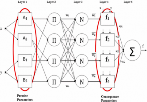
ANFIS strategy utilizes the Takagi-Sugeno structure in order to explain the nonlinear reliance of inputted data and the results [60]. A schematic of the ANFIS structure is presented in Figure 1. Suppose a system with two inputs of X1 and X2, in an ordinary ANFIS structure, if-then principles will be defined as:
f1=m1X1+n1X2+r1 (4)
f2=m2X1+n2X2+r2 (5)
f3=m3X1+n3X2+r3 (6)
f4=m4X1+n4X2+r4 (7)
where f demonstrate outputs and for i=1 and i=2, Ai and Bi represent logic sets for inputted X1 and X2 parameters and is supposed that in for each output (f) logic sets be equal to the inputted data. The whole nodes in the first layer are considered to be adaptive. The layer 1’s outputs are the inputs’ fuzzy membership grade, which are provided with:
$\boldsymbol{O}_{i}^{1}=\boldsymbol{\mu}_{A_{i}}(\boldsymbol{x}) \quad \boldsymbol{i}=\mathbf{1}, \mathbf{2}$ (8)
$O_{i}^{1}=\mu_{B_{i-2}}(y) \quad i=3,4$(9)
where O is representing the output. In present work the Gaussian membership was used. An optimization procedure is necessary to optimize the parameters of membership functions. The nodes in the second layer are considered to be fixed. Their label M indicates which they operate as a simple multiplier. The following equation (10) expresses the outputs of this layer:
$\boldsymbol{o}_{i}^{2}=\boldsymbol{w}_{i}=\boldsymbol{\beta}_{A i}(\boldsymbol{x}) \boldsymbol{\beta}_{B i}(\boldsymbol{y}) \quad \mathbf{i}=\mathbf{1}, 2$ (10)
$O_{i}^{2}$ is the so-called firing strengths of the rules. The nodes in the third layer are also considered to be fixed. Their label N indicates which they perform a normalization role to the firing strengths from the previous layer:
$O_{i}^{3}=\overline{w}_{i}=\frac{w_{i}}{\sum_{i} w_{i}} \quad_{i=1,2}$ (11)
The nodes in the fourth layer are considered to be adaptive. The normalized firing strength and a first order polynomial’s product (for a first order Sugeno model) is the output of each node in this layer. Therefore, this layer’s outputs can be provided by:
$O_{i}^{4}=\overline{w}_{i} f_{i}=\overline{w}_{i}\left(a_{i} X_{1}+b_{i} X_{2}+c_{i}\right)$ (12)
The only one single fixed node exists in the fifth layer labeled with S. All incoming signals’ summation is performed with the help of this node. Thus, the following equation describes the model’s overall output:
$O_{i}^{\mathrm{S}}=\sum_{i} \overline{w}_{i} f_{i}=\frac{\Sigma_{i} w_{i} f_{i}}{\Sigma_{i} w_{i}}$ (13)
Figure 1. Typical structure of the ANFIS
2.3 Least squares support vector machine (LSSVM)
In function estimation and pattern recognition problems, support vector machines are so favorable. It is a supervised learning system which is used to classify and analyze data. The SVM method uses a function which is given by:
$f(x)=w^{T}(x) \varphi(x)+b$ (14)
b and ω and are a constant coefficient and weight vector which are obtained from the data of training step. Below equations are used to determine their optimal value [61].
$M i n=\frac{1}{2} w^{T}+c \sum_{n=1}^{N}\left(\xi_{n}-\xi_{n}^{*}\right)$ (15)
where “Min” is the cost function. With the end goal of calculating the most precise results, minimization of the cost function is needed. Equation 16 represents the constraints which are applied to the cost function:
$\left\{\begin{array}{l}{y_{n}-w^{\tau} \varphi\left(x_{n}\right)-b \leq \varepsilon+\xi_{n}, n=1,2, \ldots, N} \\ {w^{T} \varphi\left(x_{n}\right)+b-y_{n} \leq \varepsilon+\xi_{n}^{*}, n=1,2, \ldots, N} \\ {\xi_{n}, \xi_{n}^{*} \geq 0}\end{array}\right.$ (16)
where nth input is denoted by xn and its output is expressed by yn. ε is the maximum acceptable error for the function, and $\xi_{n}$ and $\xi_{n}^{*}$ show the margin of acceptable error.
Suykenes and Vandewalle did a modification on the SVM method in order to reach the result more easily than by an SVM method. They developed the least squares SVM model [62]. In their method the cost function was changed as follows:
$C=\frac{1}{2} w^{T} w+\frac{1}{2} \gamma \sum_{n=1}^{N} e_{n}^{2}$ (17)
And applied constraint was defined as:
$y_{n}=w^{T} \varphi\left(x_{n}\right)+b+e_{n}$ (18)
where enis the error variable and γ is the tuning function. Additionally, The Lagrangian function for this method can be defined as:
$L(w, b, e . a)=\frac{1}{2} w^{T} w+\frac{1}{2} \gamma \sum_{n=1}^{N} e_{n}^{2}-\sum_{n=1}^{N} a_{n}\left(w^{T} \varphi\left(x_{n}\right)+b+e_{n}-y_{n}\right)$ (19)
where An is Lagrangian coefficients. Eventually, the results of the optimization procedures are determined by:
$\left\{\begin{array}{l}{\frac{\partial L}{\partial w}=0 \Rightarrow w=\sum_{n=1}^{N} a_{n} \varphi\left(x_{n}\right)} \\ {\frac{\partial L}{\partial b}=0 \Rightarrow \sum_{n=1}^{N} a_{n}=0} \\ {\frac{\partial L}{\partial \epsilon_{n}}=0 \Rightarrow a_{k n}=\gamma e_{n}, n=1,2, \ldots, N} \\ {\frac{\partial L}{\partial a_{n}}=0 \Rightarrow w^{T} \varphi\left(x_{n}\right)+b+e_{n}-y_{n}=0, n=1,2, \ldots, N}\end{array}\right.$ (20)
The radial basis function (RBF) must be determined to complete the tuning procedure. The current study utilizes the following equation as RB function:
$k\left(x, x_{k}\right)=\exp \left(-\frac{\left\|x_{k}-x\right\|^{2}}{\sigma^{2}}\right)$ (21)
In this equation tuning of σ2 and in addition to that, optimization of γ are needed. In this point with the aim of optimization, the differences between real and estimated values must be minimized:
$M S E=\frac{1}{N} \sum_{i=1}^{N}\left(H_{i}^{e x p .}-H_{i}^{c a l .}\right)^{2}$ (22)
where in this formulation N represents the number of values? Figure 2 depicts a schematic structure of the PSO-LSSVM approach.
Figure 2. A schematic illustration of PSO-LSSVM
2.4 RBF-ANN
The configuration of an RBF-ANN system is similar to the structure of MLP-ANN, but a complex RBF function is applied to the hidden layers. The result of RBF-ANN is:
$y_{i}(x)=\sum_{k=1}^{h} w_{k i} \emptyset\left(\left\|x-c_{k}\right\|\right)$ (23)
where x is an input pattern, yi(x) is i th output, wkiis the weight of connection from the kth interior element to the ith element of outcome layer. ‖ ‖ represents the Euclidean norm and ck is the archetype of the middle of the kth interior element. Conventionally, the RBF (φ) is picked out as the Gaussian operator which is presented below.
$h(x)=\operatorname{expa}\left(-\frac{(x-c)^{2}}{r^{2}}\right)$ (24)
The radius (r) and center (c) are parameters of Gaussian RBF. Away from the center, it decreases uniformly. Vice versa, a multi quadric RBF increases uniformly with distance from the center (see Eq. 25).
$h(x)=\frac{\sqrt{r^{2}+(x-c)^{2}}}{r}$ (25)
3.1 Pre-analysis phase
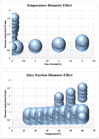
In the current paper, three analysis and model building procedures were applied for estimating the nanofluid’s thermal conductivity. Figure 3 shows the bubble curve of thermal conductivity versus the mass fraction and temperature in which the size of each bubble is dependent on the size of particles. Resulted data form experimental section of the study at the first step are used to train the models. Just about 25 % of data are used to test the models. A normalization process according to the equation 26 was done to normalize data:
$D_{k}=2 \frac{x-x_{\min }}{x_{\max }-x_{\min }}-1$ (26)
where x is the value of the nth parameter. The absolute value of Dk will be less than unity. The other values are fed to the neural network systems and the models are built to predict the thermal conductivity as the main output.
Figure 3. Bubble curves of suggested experimental data set
3.2 Outlier detection
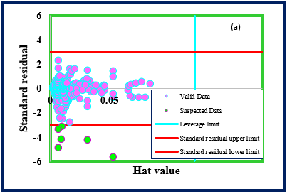
On the condition of implementing statistical approaches or training machine learning algorithms, outliers or anomalies could be mentioned as a severe concern. They are generally made due to the measurements’ errors or excellent systems conditions, as the result cannot illustrate the prevailing functioning of the underlying system. Certainly, applying an outlier removal phase before proceeding with additional investigation can be stated as the exceptional practice. The leverage value procedure applied as an outlier detection method in this study. The Hat and the residual values of any input were calculated. The following formulation applied to calculate the Hat matrix:
$H=X\left(X^{T} X\right)^{-1} X^{T}$ (27)
X is a matrix of size N×P, where N represents the total number of data points and P denotes the number of input parameters. T and -l are transposed and inverse operators, respectively. The standardized residual value of each data point calculated and employed to plot standardized values versus hat values, called Williams plot. A warning leverage value is also defined using the following expression:
$H^{*}=\frac{3(P+1)}{N}$ (28)
A rectangular area restricted to R=±3 and 0≤H≤H* is considered as the feasible region.
3.3 Model development and verification methodology
In order develop corresponding models pre-mentioned methods (MLP-ANN, LSSVM and ANFIS) were used and the models accuracy were examined Using statistical approaches. Three main evaluating parameters were used to calculate the error and estimate the accuracy of the results. Equations 29 to 33 are some of these methods that are used in the present study. All of them are used to evaluate the proposed models by measuring the differences between real and modelled data.
$M S E=\frac{1}{N} \sum_{j=1}^{N}\left(X_{j}^{r e a l}-X_{j}^{m o d}\right)^{2}$ (29)
$A R D(\%)=\frac{100}{N} \sum_{j=1}^{N} \frac{\left|X_{j}^{r e a l}-X_{j}^{m o d d}\right|}{X_{j}^{m o d}}$ (30)
$S T D=\left(\frac{1}{N-1} \sum_{j=1}^{N}\left(X_{j}^{r e a l}-X_{j}^{m o d}\right)^{2}\right)^{0.5}$ (31)
$R M S E=\left(\frac{1}{N} \sum_{f=1}^{N}\left(X_{j}^{r e a l}-X_{j}^{m o d .}\right)^{2}\right)^{0.5}$ (32)
$R^{2}=1-\frac{\sum_{j=1}^{N}\left(x_{j}^{r e a t}-x_{j}^{m o d}\right)^{2}}{\sum_{j=2}^{N}\left(x_{j}^{r e a l}-x^{r e a l}\right)^{2}}$ (33)
where X is a property, N shows the total data points, real. is a notation for experimental values and mod. is showing the modelled values. $\overline{X}^{r e a l}$ is the mean value of experimentally calculate thermal conductivity.
The proposed MLP-ANN, RBF-ANN, ANFIS, and LSSVM strategies were associated with common optimization algorithms like Levenberg Marquardt and particle swarm optimization (PSO). The detailed information of MLP-ANN including the number of neurons in hidden and output layers are listed in Table 1.
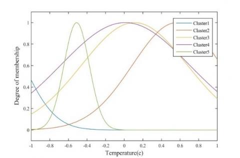
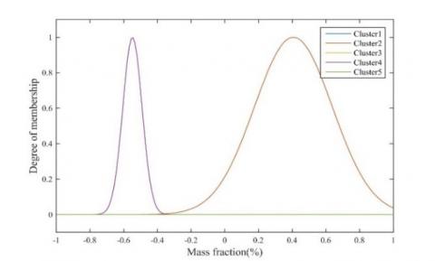
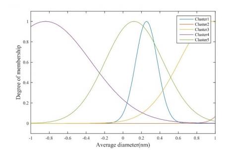
In this table the amount of weight parameter for different inputs (temperature, mass fraction and diameter of CNTs) and also the bias numbers for the interior and the output layers is presented. In association with ANFIS strategy, the particle swarm optimization (PSO) method is utilized to determine optimum parameters. Training results of membership functions for different parameters and various clusters are demonstrated in Figure 4, where the plot of degree of membership versus average diameter of particles, mass fraction and temperature are illustrated. Detailed information about the proposed models such as used membership and activation functions, number of clusters, interior and exterior layers and the optimization methods are reported in Table 2. Two kind of tuning parameters (γ and σ2) were used in the LSSVM machine. The optimized values for γ and σ2 are 57857.45 and 0.25784, respectively.
Figure 4. The trained membership functions for different input parameters
Table 1. Optimal weight and bias values for the MLP-ANN method
|
|
Hidden layer |
Output layer |
||||
|
|
Weight |
Bias |
Weight |
Bias |
||
|
Neuron |
Temperature |
Mass fraction |
Diameter |
b1 |
K |
b2 |
|
1 |
0.394618 |
4.957805 |
4.940364 |
-6.02809 |
-1.80586 |
48.5559 |
|
2 |
-7.68724 |
-7.61198 |
-2.54537 |
9.047065 |
0.152903 |
|
|
3 |
-0.86057 |
80.07941 |
-52.7706 |
28.08972 |
1.193638 |
|
|
4 |
0.008949 |
0.055302 |
3.624039 |
-5.54485 |
51.70556 |
|
|
5 |
-1.54882 |
-18.373 |
11.9616 |
-5.14446 |
-0.72265 |
|
|
6 |
120.1593 |
-119.734 |
106.5318 |
26.70881 |
0.205017 |
|
Table 2. Evaluating the performance of proposed models using statistical analysis
|
Model |
Data set |
R2 |
MRE (%) |
MSE |
RMSE |
STD |
|
ANFIS |
Train |
0.981 |
3.841 |
0.004 |
0.063 |
0.051 |
|
Test |
0.979 |
3.493 |
0.003 |
0.053 |
0.044 |
|
|
Total |
0.979 |
3.756 |
0.004 |
0.053 |
0.049 |
|
|
MLP-ANN |
Train |
0.989 |
2.289 |
0.002 |
0.043 |
0.036 |
|
Test |
0.997 |
2.613 |
0.001 |
0.035 |
0.027 |
|
|
Total |
0.990 |
2.369 |
0.002 |
0.035 |
0.034 |
|
|
RBF-ANN |
Train |
0.9974 |
1.0160 |
0.0003 |
0.0182 |
0.0154 |
|
Test |
0.9992 |
0.9355 |
0.0003 |
0.0162 |
0.0135 |
|
|
Total |
0.9982 |
0.9962 |
0.0003 |
0.0162 |
0.0149 |
|
|
LSSVM |
Train |
1.000 |
0.367 |
0.000 |
0.009 |
0.008 |
|
Test |
0.999 |
0.320 |
0.000 |
0.012 |
0.012 |
|
|
Total |
0.999 |
0.356 |
0.000 |
0.012 |
0.009 |
4.1 Model validation results
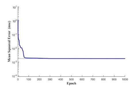
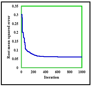
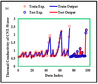
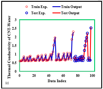
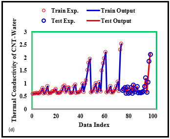
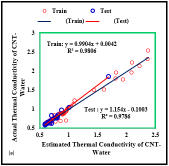
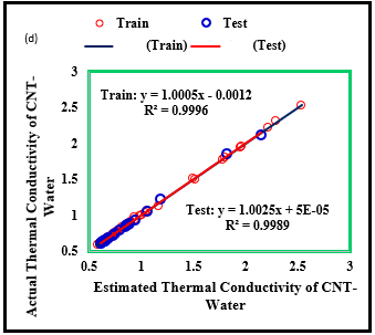
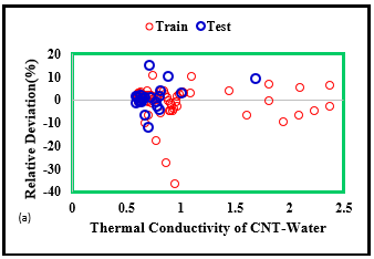
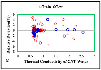
We applied both graphical and statistical approaches to evaluate the models’ performances regarding the estimation of the thermal conductivity. Figure 5 illustrates the MSE error for the MLP-ANN method. By increasing the number of iterations, MSE error was decreased to a final value of 2×10⁻³. Figure 6 demonstrate the performance of the LM algorithm to MSE for RBF-ANN approach. RBF-approach shows a more rapid decreasing in MSE than the MLP-ANN and finally gave a zero error after iteration number 30. Figure 7 shows information about the performance of ANFIS method evaluated by PSO approach. Figure 8 plots the resulted thermal conductivities obtained from proposed models. In this figure the results of prediction are plotted verses data index and shows the training and testing procedure results. From this figure in can be seen that the LSSVM and RBF-ANN had a better prediction capability and led to more precise results. The coefficient of determination (R2) indicates how close predicted values are to experimental values. This parameter usually lies between 0 and 1.0. Closer values to unity indicate more accurate predictions. Near unity coefficients of determination for proposed models, represent their capability in predicting the thermal conductivity. As is demonstrate in different parts of Figure 9, the regression diagram of experimental and estimated values shows an R2 coefficient of 0.9806 and 0.9786 for training and testing sections of the ANFIS method in part a, and in the b, c and d parts of the diagram, coefficients of determination were 0.9893& 0.9967 and 0.9974 & 0.9992 and 0.9996& 0.9989 for training and testing part of MLP-ANN, RBF-ANN and LSSVM models. The majority of data points for both training and testing datasets are concentrated around the Y=X line which implies the accurate predictions of the proposed models. In addition to the conclusion derived from figure 8, figure 9 also verifies the accurateness and the prediction capability of LSSVM and the RBF-ANN approaches. Different parts of Figure 10 illustrate the percentage of the relative deviation for developed models. It was observed that the LSSVM model had the best accuracy than the others and its relative deviation does not exceed from 5 percent band. Relative deviation of RBF-ANN also lies between +6 and -8 percent.
Figure 5. The performance of the LM algorithm according to MSE in different iterations for the MLP-ANN
Figure 6. The performance of the LM algorithm according to MSE in different iterations for the RBF-ANN
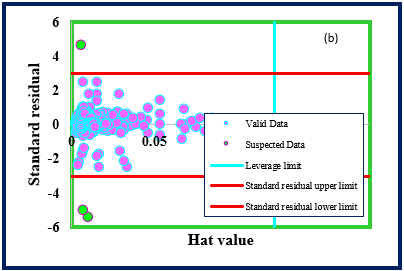
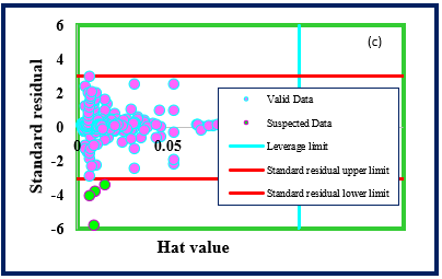
Detection of suspicious dataset for different models were done based on pre-mentioned strategy of outlier detection and results are illustrated in Figure 11. According to these analyses, based on various plots of standard residual versus Hat values, in ANFIS, MLP-ANN, RBF-ANN and LSSVM approaches 6, 3, 4 and 9 data were considered as outliers.
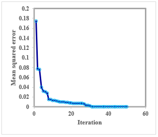
Figure 7. ANFIS performance during training stage using PSO approach
Figure 8. Estimated thermal conductivity values compared to experimental data using different models; (a) ANFIS, (b) MLP-ANN, (c) RBF-ANN, (d) LSSVM
Figure 9. Regression diagram to predict thermal conductivity using different models in the training and testing steps; (a) ANFIS, (b) MLP-ANN, (c) RBF-ANN, (d) LSSVM
Figure 10. Relative deviation (%) of testing and training data using different models; (a) ANFIS, (b) MLP-ANN, (c) RBF-ANN, (d) LSSVM
Figure 11. Detection of suspicious dataset for different models; (a) ANFIS, (b) MLP-ANN, (c) RBF-ANN, (d) LSSVM
4.2. Sensitivity analysis
A bunch of Sensitivity analyses were carried out to find out how each input parameter affects the target variable, namely the thermal conductivity. Quantitative effect of each parameter calculated using a relevancy factor defined by the following expression:
$r=\frac{\sum_{i=1}^{N}\left(x_{k, i}-z_{k}\right)\left(y_{i}-\overline{y}\right)}{\sqrt{\sum_{i=1}^{N}\left(x_{k, i}-\varepsilon_{k}\right)^{2} \sum_{i=1}^{N}\left(y_{i}-\vec{y}\right)^{2}}}$ (34)
where N, Xk,i, Yi, X̅k, Y̅ are the total number of data points, ith input value of the kth parameter, ith output value, average value of the kth input parameter, and mean value of the output parameter, respectively. The relevancy factor lays between -1 and +1 which higher absolute values represent the higher effect of the corresponding parameter. Positive effect reflects the target variable’s increment as a specific input parameter increases, while the negative effect reflects the target variable’s decrement as a specific input parameter increases. From three main input parameters, temperature and the mass fraction showed direct impact on the results; meanwhile, the average diameter showed reverse reflect on the thermal conductivity which means any increase in average diameter of CNT nanoparticles leads to reduction of thermal conductivity. Figure 12 illustrates the sensitivity analysis results, which temperature had the highest positive effects with relevancy factor of 0.67.
Figure 12. Sensitivity analysis to determine the effect of inputs on thermal conductivity
Enhancement of heat transfer rates with the lowest utilization of energy attracted a lot of attention during recent decades. Carbon nanotubes (CNTs) are considered as promising nanomaterials and have been in the center of attention. In the present study, four soft computing based approaches including MLP-ANN, ANFIS and LSSVM and RBF-ANN were used in order to model the amount of thermal conductivity of CNT-Water nanofluid system. Among MLP-ANN, ANFIS and LSSVM and RBF-ANN methods, it was found that the LSSVM produced better results with the lowest deviation factor and reflected the most accurate responses. The regression diagram of experimental and estimated values shows the R2 coefficient of 0.9806 and 0.9789 for training and testing sections of the ANFIS method in part a, and also in the b, c and d parts of the diagram, coefficients of determination were 0.9893& 0.9967 and 0.9974 & 0.9992 and 0.9996& 0.9989 for training and testing part of MLP-ANN, RBF-ANN and LSSVM models. Furthermore, LSSVM model had the best accuracy than the others and its relative deviation does not exceed from 5 percent band. Relative deviation of RBF-ANN also lies between +6 and -8 percent. Results from sensitivity analysis revealed that temperature and the mass fraction had direct impact on the results; meanwhile, the average diameter showed reverse reflect on the thermal conductivity which means any increase in average diameter of CNT nanoparticles leads to reduction of thermal conductivity. The Presented study can be worthy to reach a better understanding of nanofluids and their applications in heat transfer phenomenon especially when a high level of performance is needed.
|
B |
dimensionless heat source length |
|
CP |
specific heat, J. kg-1. K-1 |
|
g k |
gravitational acceleration, m.s-2 thermal conductivity, W.m-1. K-1 |
|
Nu |
local Nusselt number along the heat source |
|
Greek symbols
|
|
|
a |
thermal diffusivity, m2. s-1 |
|
b |
thermal expansion coefficient, K-1 |
|
f |
solid volume fraction |
|
Ɵ |
dimensionless temperature |
|
µ |
dynamic viscosity, kg. m-1.s-1 |
|
Subscripts
|
|
|
p |
nanoparticle |
|
f |
fluid (pure water) |
|
nf |
nanofluid |
[1] Ahmadi, M.H., Tatar, A., Seifaddini, P., Ghazvini, M., Ghasempour, R., Sheremet, M.A. (2018). Thermal conductivity and dynamic viscosity modeling of Fe2O3 /water nanofluid by applying various connectionist approaches. Numer Heat Transf Part A, 4: 1301-22. https://doi.org/10.1080/10407782.2018.1505092
[2] Esfe, M.H., Rostamian, H., Esfandeh, S., Afrand, M. (2018). Modeling and prediction of rheological behavior of Al2O3-MWCNT/5W50 hybrid nano-lubricant by artificial neural network using experimental data. Physica A: Statistical Mechanics and its Applications, 510: 625-634. https://doi.org/10.1016/J.PHYSA.2018.06.041
[3] Esfe, M.H., Kamyab, M.H., Afrand, M., Amiri, M.K. (2018). Using artificial neural network for investigating of concurrent effects of multi-walled carbon nanotubes and alumina nanoparticles on the viscosity of 10W-40 engine oil. Physica A: Statistical Mechanics and its Applications, 510: 610-624. https://doi.org/10.1016/J.PHYSA.2018.06.029
[4] Motevasel, M., Nazar, A.R.S., Jamialahmadi, M. (2017). Experimental investigation of turbulent flow convection heat transfer of MgO/water nanofluid at low concentrations–Prediction of aggregation effect of nanoparticles. International Journal of Heat and Technology, 35(4): 755-764. https://doi.org/10.18280/ijht.350409
[5] Nasrin, R., Alim, M. (2015). Thermal performance of nanofluid filled solar flat plate collector. Int J Heat Technol, 33: 17-24. https://doi.org/10.18280/ijht.330203
[6] Rahman, M.M., Aziz, A. (2012). Heat transfer in water based nanofluids (TiO2-H2O, Al2O3-H2O and Cu-H2O) over a stretching cylinder. International Journal of Heat and Technology, 30: 43-49. https://doi.org/10.18280/ijht.300205
[7] Mukherjee, S., Mishra, P.C. (2018). Theoretical modeling and optimization of microchannel heat sink cooling with TiO2-water and ZnO-water nanofluids. International Journal of Heat and Technology, 36: 165-172.
[8] Ajeel, R.K., Salim, W.S.W. (2018). Numerical investigations of flow and heat transfer enhancement in a semicircle zigzag corrugated channel using nanofluids. International Journal of Heat and Technology, 36: 1292-1303.
[9] Esfe, M.H., Nadooshan, A.A., Arshi, A., Alirezaie, A. (2018). Convective heat transfer and pressure drop of aqua based TiO2 nanofluids at different diameters of nanoparticles: Data analysis and modeling with artificial neural network. Phys E Low-Dimensional Syst Nanostructures, 97: 155-161. https://doi.org/10.1016/J.PHYSE.2017.10.002
[10] Esfe, M.H., Tatar, A., Ahangar, M.R.H., Rostamian, H. (2018). A comparison of performance of several artificial intelligence methods for predicting the dynamic viscosity of TiO2/SAE 50 nano-lubricant. Phys E Low-Dimensional Syst Nanostructures, 96: 85-93. https://doi.org/10.1016/J.PHYSE.2017.08.019
[11] Esfe, M.H., Rostamian, H., Sarlak, M.R., Rejvani, M., Alirezaie, A. (2017). Rheological behavior characteristics of TiO2-MWCNT/10w40 hybrid nano-oil affected by temperature, concentration and shear rate: An experimental study and a neural network simulating. Phys E Low-Dimensional Syst Nanostructures, 94: 231-40. https://doi.org/10.1016/J.PHYSE.2017.07.012
[12] Afrand, M., Esfe, M.H., Abedini, E., Teimouri, H. (2017). Predicting the effects of magnesium oxide nanoparticles and temperature on the thermal conductivity of water using artificial neural network and experimental data. Phys E Low-Dimensional Syst Nanostructures, 87: 242-247. https://doi.org/10.1016/J.PHYSE.2016.10.020
[13] Karimipour, A., Esfe, M.H., Safaei, M.R., Semiromi, D.T., Jafari, S., Kazi, S.N. (2014). Mixed convection of copper–water nanofluid in a shallow inclined lid driven cavity using the lattice Boltzmann method. Phys A Stat Mech Its Appl, 402: 150-168. https://doi.org/10.1016/J.PHYSA.2014.01.057
[14] Bahrami, M., Akbari, M., Bagherzadeh, S.A., Karimipour, A., Afrand, M., Goodarzi, M. (2019). Develop 24 dissimilar ANNs by suitable architectures & training algorithms via sensitivity analysis to better statistical presentation: Measure MSEs between targets & ANN for Fe–CuO/Eg–Water nanofluid. Phys A Stat Mech Its Appl, 519: 159-168. https://doi.org/10.1016/J.PHYSA.2018.12.031
[15] Akhilesh, M., Santarao, K., Babu, M.V.S. (2018). Thermal conductivity of CNT-wated nanofluids: a review. Mechanics and Mechanical Engineering, 22(1): 207-220.
[16] Vafaei, M., Afrand, M., Sina, N., Kalbasi, R., Sourani, F., Teimouri, H. (2017). Evaluation of thermal conductivity of MgO-MWCNTs/EG hybrid nanofluids based on experimental data by selecting optimal artificial neural networks. Phys E Low-Dimensional Syst Nanostructures, 85: 90-96. https://doi.org/10.1016/J.PHYSE.2016.08.020
[17] Nafchi, P.M., Karimipour, A., Afrand, M. (2019). The evaluation on a new non-Newtonian hybrid mixture composed of TiO2/ZnO/EG to present a statistical approach of power law for its rheological and thermal properties. Phys A Stat Mech Its Appl, 516: 1-18. https://doi.org/10.1016/J.PHYSA.2018.10.015
[18] Godson, L., Raja, B., Lal, D.M., Wongwises, S. (2010). Enhancement of heat transfer using nanofluids—An overview. Renew Sustain Energy Rev, 14: 629-641. https://doi.org/10.1016/J.RSER.2009.10.004
[19] Hussein, A.M., Sharma, K.V., Bakar, R.A., Kadirgama, K. (2014). A review of forced convection heat transfer enhancement and hydrodynamic characteristics of a nanofluid. Renew Sustain Energy Rev, 29: 734-743. https://doi.org/10.1016/J.RSER.2013.08.014
[20] Ghanbarpour, M., Haghigi, E.B., Khodabandeh, R. (2014). Thermal properties and rheological behavior of water based Al2O3 nanofluid as a heat transfer fluid. Exp Therm Fluid Sci, 53: 227-235. https://doi.org/10.1016/J.EXPTHERMFLUSCI.2013.12.013
[21] Huminic, G., Huminic, A. (2012). Application of nanofluids in heat exchangers: A review. Renew Sustain Energy Rev, 16: 5625-5638. https://doi.org/10.1016/J.RSER.2012.05.023
[22] Elias, M.M., Shahrul, I.M., Mahbubul, I.M., Saidur, R., Rahim, N.A. (2014). Effect of different nanoparticle shapes on shell and tube heat exchanger using different baffle angles and operated with nanofluid. Int J Heat Mass Transf, 70: 289-297. https://doi.org/10.1016/J.IJHEATMASSTRANSFER.2013.11.018
[23] Anoop, K., Cox, J., Sadr, R. (2013). Thermal evaluation of nanofluids in heat exchangers. Int Commun Heat Mass Transf, 49: 5-9. https://doi.org/10.1016/J.ICHEATMASSTRANSFER.2013.10.002
[24] Murshed, S.M.S., De Castro, C.A.N. (2014). Superior thermal features of carbon nanotubes-based nanofluids–A review. Renew Sustain Energy Rev, 37: 155-167. https://doi.org/10.1016/j.rser.2014.05.017
[25] Salaway, R.N., Zhigilei, L.V. (2014). Molecular dynamics simulations of thermal conductivity of carbon nanotubes: Resolving the effects of computational parameters. International Journal of Heat and Mass Transfer, 70: 954-964. https://doi.org/10.1016/J.IJHEATMASSTRANSFER.2013.11.065
[26] Chen, L., Xie, H. (2010). Surfactant-free nanofluids containing double- and single-walled carbon nanotubes functionalized by a wet-mechanochemical reaction. Thermochim Acta, 497: 67-71. https://doi.org/10.1016/J.TCA.2009.08.009
[27] Sarkar, S., Ganguly, S. (2015). Fully developed thermal transport in combined pressure and electroosmotically driven flow of nanofluid in a microchannel under the effect of a magnetic field. Microfluid Nanofluidics, 18: 623-636. https://doi.org/10.1007/s10404-014-1461-4.
[28] Oztop, H.F., Abu-Nada, E. (2008). Numerical study of natural convection in partially heated rectangular enclosures filled with nanofluids. Int J Heat Fluid Flow, 29: 1326-1336. https://doi.org/10.1016/J.IJHEATFLUIDFLOW.2008.04.009
[29] Selimefendigil, F., Öztop, H.F. (2015). Numerical investigation and reduced order model of mixed convection at a backward facing step with a rotating cylinder subjected to nanofluid. Comput Fluids, 109: 27-37. https://doi.org/10.1016/J.COMPFLUID.2014.12.007
[30] Sheikholeslami, M., Gorji-Bandpy, M., Ganji, D.D. (2013). Numerical investigation of MHD effects on Al2O3–water nanofluid flow and heat transfer in a semi-annulus enclosure using LBM. Energy, 60: 501-510. https://doi.org/10.1016/J.ENERGY.2013.07.070
[31] Hamad, M.A.A., Pop, I., Md Ismail, A.I. (2011). Magnetic field effects on free convection flow of a nanofluid past a vertical semi-infinite flat plate. Nonlinear Anal Real World Appl, 12: 1338-1346. https://doi.org/10.1016/J.NONRWA.2010.09.014
[32] Selimefendigil, F., Öztop, H.F. (2014). Numerical study of MHD mixed convection in a nanofluid filled lid driven square enclosure with a rotating cylinder. Int J Heat Mass Transf, 78: 741-754. https://doi.org/10.1016/J.IJHEATMASSTRANSFER.2014.07.031
[33] Sarkar, S., Ganguly, S., Biswas, G. (2014). Buoyancy driven convection of nanofluids in an infinitely long channel under the effect of a magnetic field. Int J Heat Mass Transf, 2014: 71: 328-340. https://doi.org/10.1016/J.IJHEATMASSTRANSFER.2013.12.033
[34] Selimefendigil, F., Öztop, H.F. (2014). Pulsating nanofluids jet impingement cooling of a heated horizontal surface. Int J Heat Mass Transf, 69: 54-65. https://doi.org/10.1016/J.IJHEATMASSTRANSFER.2013.10.010
[35] Piratheepan, M., Anderson, T.N. (2014). An experimental investigation of turbulent forced convection heat transfer by a multi-walled carbon-nanotube nanofluid. Int Commun Heat Mass Transf, 57: 286-290. https://doi.org/10.1016/J.ICHEATMASSTRANSFER.2014.08.010
[36] Kamali, R., Binesh, A.R. (2010). Numerical investigation of heat transfer enhancement using carbon nanotube-based non-Newtonian nanofluids. Int Commun Heat Mass Transf, 37: 1153-1157. https://doi.org/10.1016/J.ICHEATMASSTRANSFER.2010.06.001
[37] Rahman, M.M., Mojumder, S., Saha, S., Mekhilef, S., Saidur, R. (2014). Effect of solid volume fraction and tilt angle in a quarter circular solar thermal collectors filled with CNT–water nanofluid. Int Commun Heat Mass Transf, 57: 79-90. https://doi.org/10.1016/J.ICHEATMASSTRANSFER.2014.07.005
[38] Ding, Y., Alias, H., Wen, D., Williams, R.A. (2006). Heat transfer of aqueous suspensions of carbon nanotubes (CNT nanofluids). Int J Heat Mass Transf, 49: 240-250. https://doi.org/10.1016/j.ijheatmasstransfer.2005.07.009.
[39] Wang, J., Zhu, J., Zhang, X., Chen, Y. (2013). Heat transfer and pressure drop of nanofluids containing carbon nanotubes in laminar flows. Exp Therm Fluid Sci, 44: 716-721. https://doi.org/10.1016/J.EXPTHERMFLUSCI.2012.09.013
[40] Alimoradi, A., Veysi, F. (2016). Prediction of heat transfer coefficients of shell and coiled tube heat exchangers using numerical method and experimental validation. Int J Therm Sci, 107: 196-208. https://doi.org/10.1016/J.IJTHERMALSCI.2016.04.010.
[41] Ahmadi, M.H., Hajizadeh, F., Rahimzadeh, M.J., Shafii, M.B., Chamkha, A.J. (2018). Application GMDH artificial neural network for modeling of Al2O3 / water and Al2O3 / Ethylene glycol thermal conductivity 2018.
[42] Ahmadi, M.H., Nazari, M.A., Ghasempour, R., Madah, H., Shafii, M.B., Ahmadi, M.A. (2018). Thermal conductivity ratio prediction of Al2O3/water nanofluid by applying connectionist methods. Colloids Surfaces a Physicochem. Eng. Asp, 541: 154-164. https://doi.org/10.1016/J.COLSURFA.2018.01.030
[43] Ahmadi, M.H., Ahmadi, M.A., Nazari, M.A., Mahian, O., Ghasempour, R. (2019). A proposed model to predict thermal conductivity ratio of Al2O3/EG nanofluid by applying least squares support vector machine (LSSVM) and genetic algorithm as a connectionist approach. J Therm Anal Calorim, 135: 271-281. https://doi.org/10.1007/s10973-018-7035-z
[44] Baghban, A., Jalali, A., Shafiee, M., Ahmadi, M.H., Chau, K. (2019). Developing an ANFIS-based swarm concept model for estimating the relative viscosity of nanofluids. Eng. Appl. Comput. Fluid Mech, 13: 26-39. https://doi.org/10.1080/19942060.2018.1542345
[45] Ahmadi, M.A., Ahmadi, M.H., Alavi, M.F., Nazemzadegan, M.R., Ghasempour, R., Shamshirband, S. (2018). Determination of thermal conductivity ratio of CuO/ethylene glycol nanofluid by connectionist approach. J Taiwan Inst Chem Eng., 91: 383-395. https://doi.org/10.1016/J.JTICE.2018.06.003
[46] Xing, M., Yu, J., Wang, R. (2015). Experimental study on the thermal conductivity enhancement of water based nanofluids using different types of carbon nanotubes. Int J Heat Mass Transf., 88: 609-616. https://doi.org/10.1016/J.IJHEATMASSTRANSFER.2015.05.005
[47] Farbod, M., Ahangarpour, A., Etemad, S.G. (2015). Stability and thermal conductivity of water-based carbon nanotube nanofluids. Particuology, 22: 59-65. https://doi.org/10.1016/J.PARTIC.2014.07.005
[48] Sabiha, M.A., Mostafizur, R.M., Saidur, R., Mekhilef, S. (2016). Experimental investigation on thermo physical properties of single walled carbon nanotube nanofluids. Int J Heat Mass Transf., 93: 862-871. https://doi.org/10.1016/J.IJHEATMASSTRANSFER.2015.10.071
[49] Glory, J., Bonetti, M., Helezen, M., Mayne-L’Hermite, M., Reynaud, C. (2008). Thermal and electrical conductivities of water-based nanofluids prepared with long multiwalled carbon nanotubes. J Appl Phys, 103: 94309. https://doi.org/10.1063/1.2908229
[50] Walvekar, R., Faris, I.A., Khalid, M. (2012). Thermal conductivity of carbon nanotube nanofluid-Experimental and theoretical study. Heat Transf. Res, 41: 145-163. https://doi.org/10.1002/htj.20405
[51] Baghban, A., Kahani, M., Nazari, M.A., Ahmadi, M.H., Yan, W.M. (2019). Sensitivity analysis and application of machine learning methods to predict the heat transfer performance of CNT/water nanofluid flows through coils. Int J Heat Mass Transf., 128: 825-835. https://doi.org/10.1016/J.IJHEATMASSTRANSFER.2018.09.041
[52] Nielsen, M.A. (2015). Neural Networks and Deep Learning 2015.
[53] Baghban, A., Kardani, M.N., Habibzadeh, S. (2017). Prediction viscosity of ionic liquids using a hybrid LSSVM and group contribution method. J Mol Liq., 236: 452-464. https://doi.org/10.1016/J.MOLLIQ.2017.04.019
[54] Baghban, A., Sasanipour, J., Haratipour, P., Alizad, M., Vafaee Ayouri, M. (2017). ANFIS modeling of rhamnolipid breakthrough curves on activated carbon. Chem Eng. Res Des, 126: 67-75. https://doi.org/10.1016/J.CHERD.2017.08.007
[55] Mohanraj, M., Jayaraj, S., Muraleedharan, C. (2015). Applications of artificial neural networks for thermal analysis of heat exchangers – A review. Int J Therm. Sci, 90: 150-172. https://doi.org/10.1016/J.IJTHERMALSCI.2014.11.030
[56] Saeedan, M., Solaimany Nazar, A.R., Abbasi, Y., Karimi, R. (2016). CFD Investigation and neutral network modeling of heat transfer and pressure drop of nanofluids in double pipe helically baffled heat exchanger with a 3-D fined tube. Appl Therm. Eng., 100: 721-729. https://doi.org/10.1016/J.APPLTHERMALENG.2016.01.125
[57] Maddah, H., Ghazvini, M., Ahmadi, M.H. (2019). Predicting the efficiency of CuO/water nanofluid in heat pipe heat exchanger using neural network. Int Commun. Heat Mass Transf., 104: 33-40. https://doi.org/10.1016/J.ICHEATMASSTRANSFER.2019.02.002
[58] Zadeh, L.A. (1965). Fuzzy sets. Inf Control, 8: 338-353. https://doi.org/10.1016/S0019-9958(65)90241-X
[59] Chang, F.J., Chang, Y.T. (2006). Adaptive neuro-fuzzy inference system for prediction of water level in reservoir. Adv Water Resour, 29: 1-10. https://doi.org/10.1016/J.ADVWATRES.2005.04.015
[60] Sugeno, M., Kang, G. (1988). Structure identification of fuzzy model. Fuzzy Sets Syst, 28: 15-33. https://doi.org/10.1016/0165-0114(88)90113-3
[61] Baghban, A., Ahmadi, M.A., Pouladi, B., Amanna, B. (2015). Phase equilibrium modeling of semi-clathrate hydrates of seven commonly gases in the presence of TBAB ionic liquid promoter based on a low parameter connectionist technique. J Supercrit Fluids, 101: 184-192. https://doi.org/10.1016/J.SUPFLU.2015.03.004
[62] Suykens, J.A.K., Vandewalle, J. (1999). Least squares support vector machine classifiers. Neural Process Lett, 9: 293-300. https://doi.org/10.1023/A:1018628609742