OPEN ACCESS
In this paper, the effect of evacuated glass cover on convective heat loss and exergetic efficiency is studied. First, the evacuated receiver tube of LS-2 parabolic trough collectoris simulated and analyzed with computational fluid dynamics (CFD). The results have good agreements with tested results. Secondly, this mentioned collector and its absorber tube are simulated without evacuated glass cover for various wind speeds and collector orientations. Finally, exergetic analysis of each case-studies are calculated and effect of wind blast and collector orientation on the exergy destruction and exergy loss are investigated. It is found that when wind blows on the convex side of the parabolic mirror, the impressibility of outlet temperature from wind speed is least than other orientations. Also, if the wind blows on the convex side of the parabolic mirror, the impressibility of outlet temperature from the variation of orientation is most than other orientations. Therefore exergy efficiency of collector will be decreases. With increasing of wind blast, the exergy loss and the destruction of collector increase. Therefore exergy efficiency of collector will be decreases. Also, using evacuated tube leads to increasing of exergy from 10 to 60 percent.
evacuated absorber tube,parabolic trough collector, exergetic efficiency, exergy destruction, exergy loss
The study of heat loss from the receiver and heat transfer from the receiver to the working fluid are very important in determining the efficiency of solar parabolic trough collector. Several researchers tried to improve the efficiency of the parabolic solar collectors. Clark [1] determined the design factors such as mirror reflectance, tube intercept factor, incident angle, absorption talent of tube, end loss factor, sun tracking errors the influence to efficiency of a parabolic trough collector. Almanza et al. [2] analyzed the receiver behavior of parabolic trough collectors in direct steam generation (DSG) under different experimental conditions. Odeh et al. [3] investigated the performance of solar parabolic trough collector with synthetic oil and water as working fluids. The formulations for efficiency of concentrating collectors have been expanded based on absorber tube temperature to calculate the efficiency of the collector with any working fluid. Also, the numerical studies on the free convection (thermosiphon phenomenon) in a vertical annulus were studied by Wei and Tao in 1996. Then, Yoo and Cheng carried out numerical study about free convection around absorber tube in 1998 and 1999.
In 1998, Hamed and Khan and in 2000 Mota et al. investigated the natural convection in vertical porous annulus. In 2002 Shahraki [4] analyzed the fluid dynamic and heat transfer of two-dimensional buoyancy-driven flows in annular vertically pipesvia finite element method. Recently, a lot of researchers have been performed for all kinds of solar receivers. Then, in 2006 Yaghoubi et al. [5] investigated the wind flow around a parabolic collector and heat transfer from receiver tube numerically. In 2007 Kassem [6] surveyed the free convection heat transfer in the annular space between the circular collector tube and the glass cover in the parabolic trough collector. Moreover, in 2008, the Mont Carlo Ray Tracing method was usedto calculate radiation distribution around absorber tube of parabolic concentrators. This method was applied to study the effect of sun-shape and surface slope error by Shuai et al. [7]. The results of these studies were not sufficiently functional and general to apply as design guide to gain maximum available exergy. Bejan [8, 9] carried out the second law analysis and exergy extraction from solar collector under time-depended conditions. Kurtbas and Durmus [10] presented the exergy analysis of a new solar air heater and concluded that the efficiency of the heater increases with the air flow rate while decreases with the increasing heat transfer area. Bakos et al. [11] have concluded the variation of parabolic trough collector efficiency as a function of heat transfer, pipe diameter, solar radiation stringency and diameter of the parabolic collector.
Therefore, in the present paper, the numerical solving method will be applied to study the effect of wind speed and orientation of collector on exergy loss, destruction and efficiency of collector. Also, the effect of evacuated glass cover on exergy efficiency will be investigated.
2.1. Physical model
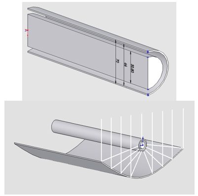
In order to study the exergetic efficiency and the destruction of exergy, LS-2 Parabolic Trough Collector is selected as a physical model. For validation of the CFD numerical method, the results will be compared with Dudley et al. [12] experimental data at Sandia National Research Laboratory (SNRL). The schematics of the absorber tube and collector are shown in Fig. 1:
Figure 1. Parabolic trough collector and the cross section of LS-2 absorber tube
The properties ofLS-2 collector and their assumptions are listed in table 1 as follow:
Table 1. The list of LS-2 PTC properties
|
LS-2 PTC (as a tested model at SANDIA research laboratory) |
|
|
Company: |
Luz industrial |
|
Operating temperature: |
100-400 ℃ |
|
Module size: |
7.8 m × 5m |
|
Rim angle: |
70 degrees |
|
Reflector: |
12 thermally sagged glass panel |
|
Aperture area: |
39.2 m2 |
|
Focal length: |
1.84 m |
|
Concentration ratio: |
22.74 |
|
Receiver: |
Evacuated tube, metal bellows at each end |
|
Diameter of Glass cover: |
115 mm |
|
Transmittance of Glass cover: |
0.95 |
|
Absorber surface: |
Cermet selective surface |
|
Absorptance: |
0.96 |
|
Absorber tube inner diameter: |
66 mm |
|
Absorber tube outer diameter: |
70 mm |
|
Flow restriction device (plug)diameter: |
50.8 mm |
Also, the used working fluid of collector is Syltherm-800 which is one of the oil derivatives. The physical and thermal properties of this working fluid are functions of temperature as shown in equations 1 to 4 as below:
$c_{\mathrm{p}}=0.00178 T+1.107798\left[\mathrm{kJ} \mathrm{kg}^{-1} \mathrm{K}^{-1}\right]$ (1)
$\rho=-0.4153495 T+1105.702\left[\mathrm{kg} \cdot \mathrm{m}^{-3}\right]$ (2)
$\mathrm{K}=-5.753496 \times 10^{-10} \mathrm{T}^{2}-1.875266 \times 10^{-4} \mathrm{T}+0.1900210$$\left[\mathrm{W} \cdot \mathrm{m}^{-1} \mathrm{K}^{-1}\right]$ (3)
$\mu=6.672 \times 10^{-13} T^{4}-1.5661 .388 \times 10^{-6} T^{2}-5.541 \times 10^{-4} T$$+8.487 \times 10^{-2}\left[\mathrm{Ns} \cdot \mathrm{m}^{-1}\right]$ (4)
These polynomial functions depend on temperature andare valid from 373.15 to 673.15 K. The stainless steel with thermal conductivity of 18 W/m K [13] is applied for the tube.
2.2 Governing equations
The governing conditions for fluid flow in the absorber tube are $k-\varepsilon$ turbulent model and steady state. So the equations that govern on the physical model are as:
Continuity equation:
$\frac{\partial}{\partial x_{\mathrm{i}}}\left(\rho u_{\mathrm{i}}\right)=0$ (5)
Momentum equation:
$\frac{\partial}{\partial x_{\mathrm{i}}}\left(\rho u_{\mathrm{i}} u_{\mathrm{j}}\right)=-\frac{\partial p}{\partial x_{\mathrm{i}}}+\frac{\partial}{\partial x_{\mathrm{i}}}\left[\left(\mu_{\mathrm{t}}+\mu\right)\left(\frac{\partial u_{\mathrm{i}}}{\partial x_{\mathrm{j}}}+\frac{\partial u_{\mathrm{j}}}{\partial x_{\mathrm{i}}}\right)-\frac{2}{3}\left(\mu_{\mathrm{t}}+\right.\right.$$\mu ) \frac{\partial u_{1}}{\partial x_{1}} \delta_{\mathrm{ij}} ]+\rho g_{\mathrm{i}}$ (6)
Energy equation:
$\frac{\partial}{\partial x_{\mathrm{i}}}\left(\rho u_{\mathrm{i}} T\right)=\frac{\partial}{\partial x_{\mathrm{i}}}\left[\left(\frac{\mu}{P r}+\frac{\mu_{\mathrm{t}}}{\sigma_{\mathrm{T}}}\right) \frac{\partial T}{\partial x_{\mathrm{i}}}\right]+S_{\mathrm{R}}$ (7)
Kinetic energy (k) equation:
$\frac{\partial}{\partial x_{\mathrm{i}}}\left(\rho u_{\mathrm{i}} k\right)=\frac{\partial}{\partial x_{\mathrm{i}}}\left[\left(\mu+\frac{\mu_{\mathrm{t}}}{\sigma_{\mathrm{k}}}\right) \frac{\partial k}{\partial x_{\mathrm{i}}}\right]+G_{\mathrm{k}}-\rho \varepsilon$ (8)
$\varepsilon$ equation:
$\frac{\partial}{\partial x_{i}}\left(\rho u_{\mathrm{i}} \varepsilon\right)=\frac{\partial}{\partial x_{\mathrm{i}}}\left[\left(\mu+\frac{\mu_{\mathrm{t}}}{\sigma_{\varepsilon}}\right) \frac{\partial \varepsilon}{\partial x_{\mathrm{i}}}\right]+\frac{\varepsilon}{k}\left(c_{1} G_{\mathrm{k}}-c_{2} \rho \varepsilon\right)$ (9)
Eventually, the turbulence viscosity and the production rate are expressed by:
$\mu_{t}=c_{\mu} \rho \frac{k^{2}}{\varepsilon}$ (10)
$G_{\mathrm{k}}=\mu_{\mathrm{t}} \frac{\partial u_{\mathrm{i}}}{\partial x_{\mathrm{j}}}\left(\frac{\partial u_{\mathrm{i}}}{\partial x_{\mathrm{j}}}+\frac{\partial u_{\mathrm{j}}}{\partial x_{\mathrm{i}}}\right)$ (11)
where the standard constants are: $C_{\mu}$=0.09, c1=1.44, c2=1.92, $\sigma_{\mathrm{k}}$=1.0, $\sigma_{\varepsilon}$=1.3, and $\sigma_{\mathrm{T}}$=0.85.
The used boundary conditions in the computational domain are as follows:
For inlet: $\dot{m}_{\mathrm{in}}=\dot{m}_{\mathrm{z}}=$ 0.6782 Kg/s (mass flow inlet), $\dot{m}_{\mathrm{x}}=\dot{m}_{\mathrm{y}}=$ 0 Kg/s, Tin=375.5 K
Turbulent kinetic energy: $k_{\mathrm{in}}=1 \% .1 / 2 u_{\mathrm{in}}^{2}$ (12)
Turbulent dissipation rate: $\varepsilon_{\mathrm{in}}=c_{\mu} \cdot \rho(T) \cdot k_{\mathrm{in}}^{2} / \mu_{\mathrm{t}}$ (13)
Considering: $c_{\mu}=0.09, \mu_{\mathrm{t}}=100[14]$ (14)
For outflow fully-developed assumption is applied. The wall of evacuated tube and experimental system is adiabatic. Also, for the tube without glass cover its wall of tube is exposed to wind and air flow and heat flux which is calculated by Mont-Carlo Ray Tracing (MCRT) method.
Solar radiation has been simulated via Mont-Carlo Ray Tracing (MCRT) as a statistical and probability method. This method is based on incident and reflection ray vectors. Since then, the finite volume methods (FVM) are used after the calculation of solar radiation distribution. Because of variation between the sun and the earth diameters, the collection of rays is considered conic shape. This optical cone osculates to one point of mirror surface. Fig. 2 shows the optical cone which is collection of several sun rays. One of sun rays in the optical cone is shown below:
Figure 2. The specification of a sun ray in the cone via two guide angles
In fig. 2 the definition of two guide angles are as:
$\theta=\tan ^{-1}\left(\sqrt{\varepsilon_{1}} \tan \theta_{\max }\right) \qquad 0 \leq \theta \leq \theta_{\max }$ (15)
$\psi=2 \pi \varepsilon_{2} \qquad 0 \leq \psi \leq 2 \pi$ (16)
Consider that, $\varepsilon_{1}$ and $\varepsilon_{2}$ are random numbers between zero and one. The collection of incident sun rays is shown with $\vec{P}$ vector that is defined as:
$\vec{P}=(\sin \theta \cos \psi,-\cos \theta, \sin \theta \sin \psi)$ (17)
Also, if sun tracking error is considered, the vector of sun ray incident is given by:
$\vec{P}=$$\left[\begin{array}{ccc}{\cos \alpha} & {-\sin \alpha} & {0} \\ {\sin \alpha} & {\cos \alpha} & {0} \\ {0} & {0} & {1}\end{array}\right]\left[\begin{array}{c}{\sin \left(\tan ^{-1}\left(\sqrt{\varepsilon_{1}} \tan \theta_{\max }\right)\right) \cos \left(2 \pi \varepsilon_{2}\right)} \\ {-\cos \tan ^{-1}\left(\sqrt{\varepsilon_{1}} \tan \theta_{\max }\right)} \\ {\sin \left(\tan ^{-1}\left(\sqrt{\varepsilon_{1}} \tan \theta_{\max }\right)\right) \sin \left(2 \pi \varepsilon_{2}\right)}\end{array}\right]$ (18)
Therefore, eq. (19) expresses the sun rays after reflection vectors.
$\vec{S}=\vec{P}-2(\vec{N} . \vec{P}) \vec{N}$ (19)
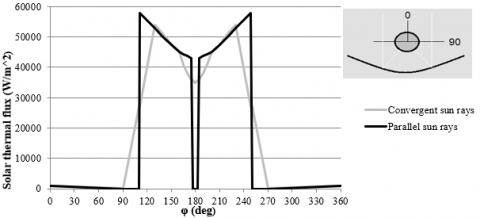
where, $\vec{N}$ is normal (orthogonal) vector on mirror surface. Therefore, the MCRT model is solved and its result is distribution of heat flux around outer wall of absorber tube. According to the local of experimental researches, the Direct Normal Incident (DNI) is considered 909.5, 928.3 and 933.7W/m2 respectively[12]. Also, fig. 3 shows the distribution of heat flux which is obtained by MCRT code versus DNI= 933.7W/ m2:
Figure 3. The solar heat flux distribution around absorber tube in LS-2 PTC
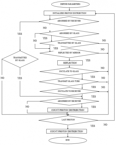
The algorithm of MCRT method for evacuated tube is shown in fig. 4. If the absorber tube is considered without glass cover, some of steps at algorithm consist of glass cover will be omitted.
After mesh generation in the tube geometry, the in-house computational code has been used to simulate the absorber tube as a receiver of radiations. The reached heat flux functions are defined and linked to main program with self-developed subroutine program. Also, the properties of Syltherm-800 are defined in code as polynomial functions. Therefore, the gravity must be activated.
The governing equations are discretized with finite volume method (FVM). Considering, the convective terms of momentum and energy are discretized with the second upwind order. The SIMPLE algorithm is applied to couple velocity and pressure together. The convergence criterion of all equations is considered less than 10-6.
The results which are obtained by simulation of LS-2 absorber tube (Dp=50.8 mm), are used to compare and validate of numerical method. Tab. 2 indicates the comparison between numerical results and Dudley's data. $\Delta T \%$ was selected as comparison criterion and its definition is as below:
$\Delta T \%=\frac{T_{\exp }-T_{\text { num }}}{T_{\text { exp }}} \times 100 \%$ (20)
The useful heat gain by the parabolic trough collector exposed to solar radiation is defined as:
$Q_{\mathrm{u}}=\dot{m} c_{\mathrm{p}}\left(T_{\mathrm{out}}-T_{\mathrm{in}}\right)$ (21)
And the thermal efficiency of the collector is obtained by:
$\eta_{\mathrm{th}}=Q_{u} /_{A_{\mathrm{c}}} . I$ (22)
where $A_{\mathrm{c}}$ is the area of the collector and I is the solar radiation incident on the collector mirror. It can be seen from table 2, there is a logical agreement between numerical and experimental results.
Figure 4. The algorithm of MCRT in MATLAB software for evacuated tube
Table 2. Comparison of outlet temperature between numerical model and Dudley's test results
|
Case study |
DNI (W/ m2)
|
Mass flow rate (kg/s) |
Inlet temperature (K) |
Outlet temperature (K) experimental |
Outlet temperature (K) numerical |
$\Delta T \%$
|
$\eta$% Efficiency experimental |
$\eta$% Efficiency numerical |
|
1 |
933.7 |
0.6782 |
375.5 |
397.5 |
399 |
0.38 |
72.07 |
74 |
|
2 |
928.3 |
0.7205 |
471 |
493 |
495.7 |
0.55 |
71 |
73.4 |
|
3 |
909.5 |
0.81 |
524.2 |
542.9 |
546.1 |
0.59 |
70.5 |
72.1 |
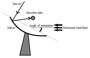
Whenthe angle of orientation becomes zero deg,the collector aperture is parallel to wind and angle of orientation becomes 90 deg means that the aperture is normal to wind. Also, The direction of wind blast is assumed horizontal. The mentioned collector is sun tracking and according to the fig. 5, the angle of orientation is defined:
Figure 5. Definition of orientation angle schematically
7.1 Average Nu
After validation, the effect of horizontal wind speed and the orientation of collector on exergy efficiency are numerically studed. Also, the influence of glass cover on prevention of exergy destruction is investigated. After simulation of each case-studies the average Nuarround absorber tube is calculated. Fig.6shows the effect of collector orientation on average Nu variation.
Figure 6. Variationdiagram of Nu around absorber tube of collector versus several orientations and wind speeds=5, 10, 15 m/sec
According to fig. 6, the maximum Nu is occurred versus orientation angle=90 deg. With decreasing of wind speed, the slope of diagrams is decreased and becomes horizontal. It means that, if the wind speed decreases, the average Nu will be constant and free convection will invigorate. Also, it is cancluded, when wind blows on the concave side of the parabolic mirror, the impressibility of average Nu from wind speed is most than other orientations.
7.2 Outlet temperature
Figure 7. Diagram of outlet temperature versus several orientations and wind speeds=5, 10, 15 m/sec
According to eq. (21) the outlet temperature (T0) is the most important in the calculation of collector thermal efficiency. Therefore, increasing of the outlet temperature leads to increasing of efficiency. Fig. 7 inhibits the impressibility of T0 from collector orientation. Considering, when wind blows on the concave side of the parabolic mirror, the impressibility of T0 from wind speed is most than other orientations. In contrast, when wind blows on the convex side of the parabolic mirror, the impressibility of T0 from wind speed is least than other orientations. Also, if the wind blows on the convex side of the parabolic mirror, the impressibility of T0 from the variation of orientation is most than other orientations. The mathematical statement of this sentence is shown in the slopes of diagrams. While, the distance between diagrams shows the impressibility of T0 from wind speeds.
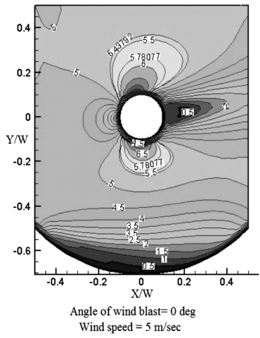
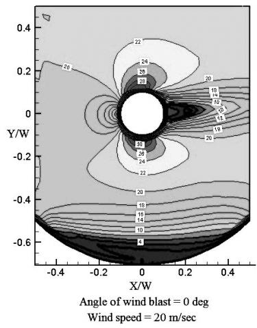
7.3 Air path lines
Typical air path lines around the absorber tube for wind speeds= 5, 10, 15 m/sec are illustrated in fig. 8 for the angle of orientation=0 deg. These schematics exhibit that several recirculation regions are made around the receiver tube. Similar results are formed when angle of orientation is increased. This figure shows that, air flow field around the receiver tube is depended on the wind speed and strongly related to the collector orientation. Heat transfer from receiver is important factor in calculating of heat loss in receiver tube. If the wind speed is very high (higher than 5 m/sec), the effect of collector on absorber tube cannot beneglected and is important. This result is concluded from fig. 7 too. In low speeds (less than 2.5 m/sec) the free convection is more effective than forced convection around absorber tube.
Figure 8. Distribution of air velocity around absorber tube versus wind speed
7.4 Exergy analysis
One of the governing equations on the solar collector is the usefull heat gain ($Q_{\mathrm{u}}$) for energy analysis. It is calculated by the working fluid property and mass flow rate as:
$Q_{\mathrm{u}}=\dot{m} c_{\mathrm{p}}\left(T_{\mathrm{out}}-T_{\mathrm{in}}\right)$ (21)
The Hottel-Whillier equation calculates theuseful heat gain for a solar collector system, considering the heat losses from the absorber tube to the ambient.Two different approaches are applied to calculate heat gain:“brute-force”, and “functional.” [15].
In a similar relation, exergy efficiency is defined as the ratio of output exergy to input exergy, as follow:
$\eta_{\mathrm{ex}}=\frac{\dot{E}_{\mathrm{out}}}{\dot{E}_{\mathrm{in}}}=1-\frac{\dot{E}_{\mathrm{dest}}}{\dot{E}_{\mathrm{in}}}$ (22)
In other definition, Exergy is determined as the maximum amount of work which can be produced by a system or flow of mass or energy as it regards to equilibrium with a reference point at surrounding[16]. Consider that, this method is used in this paper. The main form of exergy equilibrium equation is as:
$\dot{E}_{\mathrm{in}}+\dot{E}_{\mathrm{s}}+\dot{E}_{\mathrm{out}}+\dot{E}_{1}+\dot{E}_{\mathrm{dest}}=0$ (23)
where, $\dot{E}_{\mathrm{in}}, \dot{E}_{\mathrm{s}}, \dot{E}_{\mathrm{out}}, \dot{E}_{1}$ and $\dot{E}_{\mathrm{dest}}$ are the inlet, stored, outlet, loss and destroyed exergy rate, respectively. The inlet exergy rate is sum of the inlet exergy rate with fluid flow and the absorbed solar radiation exergy rate. The inlet exergy rate with fluid flow is obtained by: [16, 17]
$\dot{E}_{\mathrm{in}, \mathrm{f}}=\dot{m} c_{\mathrm{p}}\left(T_{\mathrm{in}}-T_{\mathrm{a}}-T_{\mathrm{a}} \ln \left(\frac{T_{\mathrm{in}}}{T_{\mathrm{a}}}\right)\right)+\frac{\dot{m} \Delta P_{\mathrm{in}}}{\rho}$ (24)
Also, according to the Petela theorem, the absorbed solar radiation exergy rate is calculated by: [18]
$\dot{E}_{\mathrm{in}, \mathrm{Q}}=\eta_{o} I_{\mathrm{T}} A_{\mathrm{P}}\left[1-\frac{4}{3}\left(\frac{T_{\mathrm{a}}}{T_{\mathrm{Sun}}}\right)+\frac{1}{3}\left(\frac{T_{\mathrm{a}}}{T_{\mathrm{Sun}}}\right)^{4}\right]$ (25)
The term in the bracket is named the Petela efficiency ($\eta_{\mathrm{p}}$). However, this equation contravenes the second law of thermodynamics in some systems [19]. If the sun is assumed as an infinite thermal source, the corrected form of eq. (25) will be: [19, 20]
$\dot{E}_{\mathrm{in}, \mathrm{Q}}=\eta_{\mathrm{o}} I_{\mathrm{T}} A_{\mathrm{P}}\left(1-\frac{T_{\mathrm{a}}}{T_{\mathrm{Sun}}}\right)$ (26)
where $T_{\mathrm{Sun}}$ is the apparent sun temperature and equals 75% of blackbody temperature of sun [21].
The summations of Eqs. (24) and (26) will result in total inlet exergy rate of the solar collector. The stored exergy rate is negligible at steady-state conditions. Also, the outlet exegy rate of outlet fluid flow in the solar collector is:
$\dot{E}_{\text { out }, \mathrm{f}}=-\dot{m} c_{\mathrm{p}}\left(T_{\text { out }}-T_{\mathrm{a}}-T_{\mathrm{a}} \ln \left(\frac{T_{\text { out }}}{T_{a}}\right)\right)+\frac{\dot{m} \Delta P_{\text { out }}}{\rho}$ (27)
In eqs. (24) and (27), $\Delta P_{\mathrm{in}}$ and $\Delta P_{\text { out }}$ are the pressure differences of the working fluid with the surrounding atentrance and exit of the receiver tube. The loss exergy rate consists of two terms: the first is created by heat loss rate from the absorber tube to the environment because of wind blast. It is calculated by: [22]
$\dot{E}_{1, w}=-U_{1} A_{c}\left(T_{P}-T_{a}\right)\left(1-\frac{T_{\mathrm{a}}}{T_{\mathrm{r}}}\right)$ (28)
Thesecond is created by the temperature difference between the receiver tube and the sun. In other words, the radiation loss makes these term of exergy loss: [22]
$\dot{E}_{1, \Delta \mathrm{T}_{\mathrm{S}}}=-\eta_{\mathrm{o}} I_{\mathrm{T}} A_{\mathrm{c}} T_{\mathrm{a}}\left(\frac{1}{T_{r}}-\frac{1}{T_{\mathrm{Sun}}}\right)$ (29)
where $\eta_{0}$ is optical efficiency of collector and calculated by $\eta_{0}=\tau \alpha$. The destroyed exergy rate consists of two terms: The first term is caused by the pressure drop in the receiver tube duct: [23, 24]
$\dot{E}_{\mathrm{dest}, \Delta \mathrm{p}}=-\frac{\dot{m} \Delta P}{\rho} \frac{T_{\mathrm{a}} \ln \frac{T_{\mathrm{out}}}{T_{\mathrm{a}}}}{\left(T_{\mathrm{out}}-T_{\mathrm{in}}\right)}$ (30)
And the second term is concluded by the temperature difference between the receiver tube surface and the working fluid which is obtained by: [23, 24]
$\dot{E}_{\mathrm{dest}, \Delta \mathrm{T}_{\mathrm{f}}}=-\dot{m} c_{\mathrm{p}}\left(\ln \left(\frac{T_{\mathrm{out}}}{T_{\mathrm{a}}}\right)-\frac{T_{\mathrm{out}}-T_{\mathrm{in}}}{T_{\mathrm{r}}}\right)$ (31)
Therefore, the eq. (23) is discretized to more terms as:
$\dot{E}_{\mathrm{in}, \mathrm{f}}+\dot{E}_{\mathrm{in}, \mathrm{Q}}+\dot{E}_{\mathrm{s}}+\dot{E}_{\mathrm{out}, \mathrm{f}}+\dot{E}_{1, \mathrm{w}}+\dot{E}_{1, \Delta \mathrm{T}_{\mathrm{s}}}+\dot{E}_{\mathrm{dest}, \Delta \mathrm{p}}+\dot{E}_{\mathrm{dest}, \Delta \mathrm{T}_{\mathrm{f}}}=0$ (32)
Exergy loss Exergy destruction
If the absorbed solar radiation exergy rate ($\dot{E}_{\mathrm{in}, \mathrm{Q}}$) supplants to right hand and two hands of resulted equation divided to $\dot{E}_{\mathrm{in}, \mathrm{Q}}$ then:
$\frac{\dot{E}_{\mathrm{in}, \mathrm{f}}+\dot{E}_{\mathrm{out}, \mathrm{f}}+\dot{E}_{1, \mathrm{w}}+\dot{E}_{1, \Delta \mathrm{T}_{\mathrm{S}}}+\dot{E}_{\mathrm{dest}, \Delta \mathrm{p}}+\dot{E}_{\mathrm{dest}, \Delta \mathrm{T}_{\mathrm{f}}}}{-\dot{E}_{\mathrm{in}, \mathrm{Q}}}=1$ (33)
The exergy efficiency has been defined as the increase of fluid flow exergy to the radiation source in solar collectors. In other words:
$\eta_{\mathrm{ex}}=\frac{\dot{E}_{\mathrm{in}, \mathrm{f}}+\dot{E}_{\mathrm{out}, \mathrm{f}}}{-\dot{E}_{\mathrm{in}, \mathrm{Q}}}$ (34)
Subtitlingeqs.(24), (26) and (27) into Eq. (34), the exergy efficiency of the solar collector is calculated by: [19, 22, 25]
$\eta_{\mathrm{ex}}=\frac{\dot{m}\left[c_{\mathrm{P}}\left(T_{\mathrm{out}}-T_{\mathrm{in}}-T_{\mathrm{a}} \ln \left(\frac{T_{\mathrm{out}}}{T_{\mathrm{a}}}\right)\right)-\frac{\Delta P}{\rho}\right.}{I_{T} A_{\mathrm{c}}\left(1-\frac{T_{\mathrm{a}}}{T_{\mathrm{sun}}}\right)}=1-\left\{\left(1-\eta_{\mathrm{o}}\right)+\right.$
$\frac{\dot{m} \Delta P}{\rho I_{\mathrm{T}} A_{\mathrm{C}}\left(1-\frac{T_{\mathrm{a}}}{T_{\text { sun }}}\right)} \frac{T_{\mathrm{a}} \ln \left(\frac{T_{\text { out }}}{T_{\mathrm{a}}}\right)}{\left(T_{\text { out }}-T_{\text { in }}\right)}+\frac{\eta_{0} T_{\mathrm{a}}}{1-\frac{T_{\mathrm{a}}}{T_{\text { Sun }}}}\left(\frac{1}{T_{r}}-\frac{1}{T_{\text {sun}}}\right)+\frac{U_{1}\left(T_{\mathrm{r}}-T_{\mathrm{a}}\right)}{l_{\mathrm{T}}\left(1-\frac{T_{\mathrm{a}}}{T_{\text { sun }}}\right)}(1-$
$\frac{T_{\mathrm{a}}}{T_{\mathrm{r}}} )+\frac{\dot{m c}_{\mathrm{p}} T_{\mathrm{a}}}{I_{\mathrm{T}} A_{\mathrm{C}}} \frac{\left(\ln \left(\frac{T_{\mathrm{out}}}{T_{\mathrm{in}}}\right)-\frac{\left(T_{\mathrm{out}}-T_{\mathrm{in}}\right)}{T_{r}}\right)}{\left(1-\frac{T_{\mathrm{a}}}{T_{\mathrm{sun}}}\right)} \}$ (35)
The amounts of exergy have been calculated and presented in tabs. 3, 4 and 5 for the wind speeds 5, 10 and 15 m/sec respectively. Consider that, the amounts of exergy loss, exergy destruction and exergy efficiency have been obtained separately.
Table 3. Amounts of exergy for several orientations and wind speed= 5 m/sec
|
Orientation |
$\dot{E}_{\mathrm{in}, \mathrm{Q}}$ (W) |
$\dot{E}_{\mathrm{in}, \mathrm{f}}$ (W) |
$\dot{E}_{\mathrm{s}}$ (W) |
$\dot{E}_{\mathrm{out}, \mathrm{f}}$ (W) |
$\dot{E}_{\mathrm{l}, \mathrm{w}}$ (W) |
$\dot{\boldsymbol{E}}_{\mathbf{l}, \Delta \mathbf{T}_{s}}$ (W) |
$\dot{E}_{\mathrm{dest}, \Delta \mathbf{p}}$ (W) |
$\dot{\boldsymbol{E}}_{\mathrm{dest}, \Delta \mathbf{T}_{\mathrm{f}}}$ (W) |
$\boldsymbol{\eta}_{\mathrm{ex}}$ % |
|
-90 |
+39549 |
+20345 |
$\cong 0$ |
-40259 |
-5034 |
-1471 |
-4023 |
-9103 |
50.35 |
|
-75 |
+39549 |
+20345 |
$\cong 0$ |
-39203 |
-6154 |
-1455 |
-3865 |
-9217 |
47.68 |
|
-60 |
+39549 |
+20345 |
$\cong 0$ |
-38346 |
-7056 |
-1398 |
-3650 |
-9444 |
45.52 |
|
-45 |
+39549 |
+20345 |
$\cong 0$ |
-37269 |
-8243 |
-1370 |
-3550 |
-9462 |
42.79 |
|
-30 |
+39549 |
+20345 |
$\cong 0$ |
-36593 |
-8950 |
-1356 |
-3503 |
-9492 |
41.08 |
|
-15 |
+39549 |
+20345 |
$\cong 0$ |
-36015 |
-9530 |
-1334 |
-3490 |
-9525 |
39.62 |
|
0 |
+39549 |
+20345 |
$\cong 0$ |
-34633 |
-10888 |
-1316 |
-3474 |
-9583 |
37.12 |
|
15 |
+39549 |
+20345 |
$\cong 0$ |
-34020 |
-11502 |
-1304 |
-3444 |
-9624 |
34.58 |
|
30 |
+39549 |
+20345 |
$\cong 0$ |
-32823 |
-12675 |
-1297 |
-3423 |
-9676 |
31.55 |
|
45 |
+39549 |
+20345 |
$\cong 0$ |
-31969 |
-13540 |
-1275 |
-3407 |
-9703 |
29.39 |
|
60 |
+39549 |
+20345 |
$\cong 0$ |
-31404 |
-14067 |
-1264 |
-3394 |
-9765 |
27.96 |
|
75 |
+39549 |
+20345 |
$\cong 0$ |
-30652 |
-14786 |
-1256 |
-3376 |
-9824 |
26.06 |
|
90 |
+39549 |
+20345 |
$\cong 0$ |
-30400 |
-15034 |
-1235 |
-3350 |
-9875 |
25.42 |
Table 4. Amounts of exergy for several orientations and wind speed= 10 m/sec
|
Orientation |
$\dot{E}_{\mathrm{in}, \mathrm{Q}}$ (W) |
$\dot{E}_{\mathrm{in}, \mathrm{f}}$ (W) |
$\dot{E}_{\mathrm{s}}$ (W) |
$\dot{E}_{\mathrm{out}, \mathrm{f}}$ (W) |
$\dot{E}_{\mathrm{l}, \mathrm{w}}$ (W) |
$\dot{\boldsymbol{E}}_{\mathbf{l}, \Delta \mathbf{T}_{s}}$ (W) |
$\dot{E}_{\mathrm{dest}, \Delta \mathbf{p}}$ (W) |
$\dot{\boldsymbol{E}}_{\mathrm{dest}, \Delta \mathbf{T}_{\mathrm{f}}}$ (W) |
$\boldsymbol{\eta}_{\mathrm{ex}}$ % |
|
-90 |
+39549 |
+20345 |
$\cong 0$ |
-38561 |
-6129 |
-1045 |
-3925 |
-10234 |
46.06 |
|
-75 |
+39549 |
+20345 |
$\cong 0$ |
-37171 |
-6933 |
-1259 |
-3766 |
-10765 |
42.54 |
|
-60 |
+39549 |
+20345 |
$\cong 0$ |
-36196 |
-7836 |
-1168 |
-3521 |
-11173 |
40.08 |
|
-45 |
+39549 |
+20345 |
$\cong 0$ |
-35154 |
-9006 |
-1043 |
-3459 |
-11232 |
37.44 |
|
-30 |
+39549 |
+20345 |
$\cong 0$ |
-34476 |
-9850 |
-977 |
-3304 |
-11287 |
35.73 |
|
-15 |
+39549 |
+20345 |
$\cong 0$ |
-33888 |
-10492 |
-934 |
-3277 |
-11303 |
33.21 |
|
0 |
+39549 |
+20345 |
$\cong 0$ |
-33321 |
-11180 |
-889 |
-3164 |
-11340 |
30.89 |
|
15 |
+39549 |
+20345 |
$\cong 0$ |
-31907 |
-12633 |
-843 |
-3119 |
-11392 |
29.34 |
|
30 |
+39549 |
+20345 |
$\cong 0$ |
-30283 |
-14297 |
-807 |
-3072 |
-11435 |
25.13 |
|
45 |
+39549 |
+20345 |
$\cong 0$ |
-28644 |
-16040 |
-717 |
-3007 |
-11486 |
20.98 |
|
60 |
+39549 |
+20345 |
$\cong 0$ |
-27275 |
-17545 |
-592 |
-2975 |
-11507 |
17.52 |
|
75 |
+39549 |
+20345 |
$\cong 0$ |
-25419 |
-19521 |
-482 |
-2923 |
-11549 |
13.32 |
|
90 |
+39549 |
+20345 |
$\cong 0$ |
-23025 |
-22034 |
-375 |
-2890 |
-11570 |
10.1 |
Table 5. Amounts of exergy for several orientations and wind speed= 15 m/sec
|
Orientation |
$\dot{E}_{\mathrm{in}, \mathrm{Q}}$ (W) |
$\dot{E}_{\mathrm{in}, \mathrm{f}}$ (W) |
$\dot{E}_{\mathrm{s}}$ (W) |
$\dot{E}_{\mathrm{out}, \mathrm{f}}$ (W) |
$\dot{E}_{\mathrm{l}, \mathrm{w}}$ (W) |
$\dot{\boldsymbol{E}}_{\mathbf{l}, \Delta \mathbf{T}_{s}}$ (W) |
$\dot{E}_{\mathrm{dest}, \Delta \mathbf{p}}$ (W) |
$\dot{\boldsymbol{E}}_{\mathrm{dest}, \Delta \mathbf{T}_{\mathrm{f}}}$ (W) |
$\boldsymbol{\eta}_{\mathrm{ex}}$ % |
|
-90 |
+39549 |
+20345 |
$\cong 0$ |
-36154 |
-7312 |
-971 |
-3804 |
-11653 |
39.97 |
|
-75 |
+39549 |
+20345 |
$\cong 0$ |
-35323 |
-8003 |
-913 |
-3652 |
-12003 |
37.82 |
|
-60 |
+39549 |
+20345 |
$\cong 0$ |
-34289 |
-8927 |
-878 |
-3446 |
-12354 |
35.26 |
|
-45 |
+39549 |
+20345 |
$\cong 0$ |
-33171 |
-9965 |
-822 |
-3369 |
-12567 |
32.43 |
|
-30 |
+39549 |
+20345 |
$\cong 0$ |
-32896 |
-10132 |
-795 |
-3217 |
-12854 |
30.5 |
|
-15 |
+39549 |
+20345 |
$\cong 0$ |
-31256 |
-11477 |
-731 |
-3163 |
-13267 |
27.59 |
|
0 |
+39549 |
+20345 |
$\cong 0$ |
-30436 |
-12185 |
-689 |
-3049 |
-13535 |
25.52 |
|
15 |
+39549 |
+20345 |
$\cong 0$ |
-28810 |
-13671 |
-645 |
-2935 |
-13833 |
21.4 |
|
30 |
+39549 |
+20345 |
$\cong 0$ |
-26780 |
-15430 |
-602 |
-2847 |
-14235 |
17.9 |
|
45 |
+39549 |
+20345 |
$\cong 0$ |
-24690 |
-17189 |
-577 |
-2739 |
-14699 |
12.5 |
|
60 |
+39549 |
+20345 |
$\cong 0$ |
-23102 |
-18545 |
-503 |
-2654 |
-15090 |
8.67 |
|
75 |
+39549 |
+20345 |
$\cong 0$ |
-21850 |
-19825 |
-420 |
-2545 |
-15254 |
3.81 |
|
90 |
+39549 |
+20345 |
$\cong 0$ |
-20406 |
-21120 |
-382 |
-2463 |
-15523 |
0.15 |
Since then, the all mentioned terms of exergy is calculated for evacuated tube which is used in all orientations and wind speeds. Because of evacuated glass cover, the results areindependent of orientations and wind speeds. Tab. 6 presents these results as follow:
Table 6. Amounts of exergy for several orientations and wind speeds using avacuated tube
|
All case-studies |
$\dot{E}_{\mathrm{in}, \mathrm{Q}}$ (W) |
$\dot{E}_{\mathrm{in}, \mathrm{f}}$ (W) |
$\dot{E}_{\mathrm{s}}$ (W) |
$\dot{E}_{\mathrm{out}, \mathrm{f}}$ (W) |
$\dot{E}_{\mathrm{l}, \mathrm{w}}$ (W) |
$\dot{\boldsymbol{E}}_{\mathbf{l}, \Delta \mathbf{T}_{s}}$ (W) |
$\dot{E}_{\mathrm{dest}, \Delta \mathbf{p}}$ (W) |
$\dot{\boldsymbol{E}}_{\mathrm{dest}, \Delta \mathbf{T}_{\mathrm{f}}}$ (W) |
$\boldsymbol{\eta}_{\mathrm{ex}}$ % |
|
|
+39549 |
+20345 |
$\cong 0$ |
-44563 |
≅0 |
-1621 |
-4503 |
-9207 |
61.24 |
Finally, in fig. 9, the comparative diagram of exergy efficiency has been presented for all orientations and wind speeds. Consider that, the increase of wind speed leads to increasing of exergy efficiency. Also, the variation of collector from -90 to 90 deg increases the exergy efficiency. Also, using evacuated tube leads to increasing of exergy from 10% to 60%.
Figure 9. Comparative diagram of exergy efficienciy versus several orientations and wind speeds
The maximum Nu is occurred versus orientation angle=90 deg. With decreasing of wind speed, the slope of diagrams is decreased and becomes horizontal. It means that, if the wind speed decreases, the average Nu will be constant and free convection will invigorate.
When wind blows on the concave side of the parabolic mirror, the impressibility of average Nu from wind speed is most than other orientations.
When wind blows on the concave side of the parabolic mirror, the impressibility of T0 from wind speed is most than other orientations.
When wind blows on the convex side of the parabolic mirror, the impressibility of T0 from wind speed is least than other orientations.
If the wind blows on the convex side of the parabolic mirror, the impressibility of T0 from the variation of orientation is most than other orientations.
In low speeds (less than 2.5 m/sec) the free convection is more effective than forced convection around absorber tube.
Air flow field around the receiver tube is depended on the wind speed and strongly related to the collector orientation.
The comparison of tabs. 3, 4, 5,concluded that, the orientation of collector and wind speed have more effect on $\dot{E}_{1, \mathrm{w}}$ and therefore, the exergy loss changes salient. But, the effect of orientation and wind speeds are considered negligible on radiation loss ($\dot{E}_{1, \Delta \mathrm{T}_{\mathrm{s}}}$).
The context of exergy is consist of $\dot{E}_{\mathrm{dest}, \Delta \mathrm{p}}$ and $\dot{E}_{\mathrm{dest}, \Delta \mathrm{f}}$. In other words, the pressure drop and temperature difference between the absorber tube and the agent flow lead to exergy destruction.
The orientation of collector and wind speed have negligible effect on $\dot{E}_{1, \Delta \mathrm{T}_{\mathrm{S}}}$, but, two mentioned parameters have more influence on $\dot{E}_{\mathrm{dest}, \Delta \mathrm{p}}$ and $\dot{E}_{\mathrm{dest}, \Delta \mathrm{f}}$.
With increasing of orientation angle from -90 to 90, the exergy loss and destruction increase. Therefore exergy efficiency of collector will be decreases.
With increasing of wind blast from 5 to 15, the exergy loss and destruction increase. Therefore exergy efficiency of collector will be decreases.
Using evacuated tube leads to increasing of exergy from 10% to 60%.v
a ambient
$\mathrm{c}_{\mu}, \mathrm{c}_{1}, \mathrm{c}_{2}$ coefficients in the turbulence model
$\mathrm{C}_{\mathrm{p}}$ specific heat of fluid [kJ kg-1K-1]
K thermal conductivity
Pr Prandtl number
Nu Nusselt number
$\dot{\mathrm{m}}$ mass flow rate [kg s-1]
D hydraulic diameter [m]
d diameter [m]
Q heat transfer rate [W]
$\mathrm{Q}_{\mathrm{u}}$ usefull heat gain
Re Reynolds number based on tube hydraulic diameter
$\mathrm{S}_{\mathrm{R}}$ additional source term [W m-3]
t temperature [K]
u velocity components [m s-1]
U collector loss coefficient
x, y, z Cartesian coordinates
Greek symbols
$\rho$ density [kg∙m-3]
μ dynamic viscosity [Pa s]
$\mu_{\mathrm{t}}$ turbulent viscosity [Pa s]
k kinetic energy
ɛ turbulent dissipation rate or emissivity
$\sigma_{T}$ turbulent Prandtl number
$\sigma_{k,} \sigma_{\varepsilon}$ turbulent Prandtl numbers for diffusion of k and ɛ
ν kinematic viscosity [m2 s-1]
η collector efficiency
($\tau \alpha$) effective product transmittance- absorptance
Subscripts
c collector
dest destruction
in inlet
f fluid
i, j, kunit vectors in coordination system
o optical
out outlet
m average
ex exergy
exp experimental
num numerical
r receiver tube
th thermal
T incident
w wind
W wide of collector aperture
[1] Clark JA. (1982). An analysis of the technical and economic performance of a parabolic trough concentrator for solar industrial process heat application. Int. J Heat Mass Transfer 25(9): 1427-1438.
[2] Almanza R, Lentz A, Jimenez G. (1997). Receiver behavior in direct steam generation with parabolic troughs. Sol Energy 61(4): 275-278.
[3] Odeh SD, Morrison GL, Behnia M. (1998). Modelling of parabolic through direct steam generation solar collectors. Sol Energy 62(6): 395-406.
[4] Shahraki F. (2002). Modeling of buoyancy-driven flow and heat transfer for air in a horizontal annulus: effects of vertical eccentricity and temperature-dependent properties. Numerical Heat Transfer Part A – Applications 42(6): 603-621.
[5] Naeeni N, Yaghoubi M. (2007). Analysis of wind flow around a parabolic collector (1) fluid flow. Renewable Energy 32(11): 1898-1916.
[6] Kassem T. (2007). Numerical study of the natural convection process in the parabolic-cylindrical solar collector. Desalination 209(1): 144-150.
[7] Shuai Y, Xia XL, Tan HP. (2008). Radiation performance of dish solar concentrator/cavity receiver systems. Solar Energy 82(1): 13-21.
[8] Bejan A, Kearney DW, Kreith F. (1981). Second law analysis and synthesis of solar collector systems. ASME J. Solar Energy 103: 23-28.
[9] Bejan A. (1982). Extraction of exergy from solar collectors under time-varying conditions. Int. J. Heat Fluid Flow. 3(2): 67-72.
[10] Kurtbas I, Durmus A. (2004). Efficiency and exergy analysis of a new solar air heater. Renewable Energy 29(9): 1489-1501.
[11] Bakos GC, Ioannidis I, Tsagas NF, Seftelis I. (2001). Design optimization and conversion-efficiency determination of a line-focus parabolic-trough solar collector (PTC). Applied Energy 68(1): 43-50.
[12] Dudley V, Kolb G, Sloan M, Kearney D. (1994). SEGS LS2 solar collector — test results, Report of Sandia National Laboratories. SANDIA94-1884, USA, 1994.
[13] He YL, Xiao J, Cheng ZD, Tao YB. (2011). A MCRT and FVM coupled simulation method for energy conversion process in parabolic trough solar collector. Renewable Energy 36(3): 976-985.
[14] Tao WQ. (2001). Numerical Heat Transfer, Second Ed, Xi'an Jiaotong University Press, Xi'an.
[15] DiPippo R. (2004). Second law assessment of binary plants generation power from low-temperature geothermal fluids. Geothermics 33: 565-586.
[16] Kotas TJ. (1995). The exergy method of thermal plant analysis. Malabar, FL: Krieger Publish Company, 1995.
[17] Bejan A. (1988). Advanced engineering thermodynamics. New York: Wiley Interscience 133-137, 462-465.
[18] Petela R. (1964). Exergy of heat radiation. ASME Journal of Heat Transfer 86: 187-192.
[19] Najian MR. (2000). Exergy analysis of flat plate solar collector. MS Thesis, Tehran, Iran: Department of Mechanical Engineering., College of Engineering, Tehran University, 2000.
[20] Torres-Reyes E, Cervantes de Gortari JG, Ibarra-Salazar BA, Picon-Nunez M. (2001). A design method of flat-plate solar collectors based on minimum entropy generation. Exergy 1: 46-52.
[21] Bejan A, Keary DW, Kreith F. (1981). Second law analysis and synthesis of solar collector systems. Journal of Solar Energy Engineering 103: 23-28.
[22] Dutta Gupta KK, Saha SK. (1990). Energy analysis of solar thermal collectors. Renewable Energy and Environment 283-287.
[23] Suzuki A. (1988). General theory of exergy balance analysis and application to solar collectors. Energy 13: 153-160.
[24] Suzuki A. (1988). A fundamental equation for exergy balance on solar collectors. Journal of Solar Energy Engineering 110: 102-106.
[25] Luminosu I, Fara L. (2005). Determination of the optimal operation mode of a flat solar collector by exergetic analysis and numerical simulation. Energy 30: 731-747.
[26] Cornelissen RL. (1997). Thermodynamics and sustainable development: the use of exergy analysis and the reduction of irreversibility. PhD thesis, University of Twente, The Netherland.