D. Sandhya Rani![]() | Khalid Mohiuddin
| Khalid Mohiuddin![]() | Nannaparaju Vasudha
| Nannaparaju Vasudha![]() | Kanagiri Swapna
| Kanagiri Swapna![]() | Praveen Kulkarni*
| Praveen Kulkarni*![]() | P. Naresh
| P. Naresh![]() | T. M. Rajesh
| T. M. Rajesh![]() | M. N. RenukaDevi
| M. N. RenukaDevi![]()
© 2025 The authors. This article is published by IIETA and is licensed under the CC BY 4.0 license (http://creativecommons.org/licenses/by/4.0/).
OPEN ACCESS
Customer churn prediction remains an important task for telecom service providers aiming to strengthen customer retention and reduce service attrition. In this study, a predictive framework is proposed by combining Principal Component Analysis (PCA) for dimensionality reduction with several bagged ensemble models, including Random Forest, Decision Tree, SVM, and LightGBM. The proposed models were trained using a real telecom dataset that reflects customer usage trends, service choices, and subscription histories. PCA serves to compress the feature space and eliminate data redundancy, while bagging contributes to performance stability, particularly when dealing with imbalanced classes. Among the evaluated models, LightGBM delivered the most promising results, achieving an accuracy of 80.13% and an AUC of 0.9069. These results demonstrate that PCA-supported ensemble techniques can identify meaningful churn indicators; however, the work does not compare performance against non-PCA or non-bagged variants, and therefore no superiority claims are made. The framework can assist telecom providers in understanding churn tendencies and may be further improved by integrating time-based behavioral patterns, customer feedback data, or real-time prediction capabilities in future studies.
imbalanced data, ensemble technique, bagging methods, dimensionality reduction, churn
The process of studying and determining which consumers are most likely to discontinue their service or subscription is known as churn prediction. In the current digital era, attracting new customers and keeping existing ones is essential for improving business strategies. Additionally, it is more advantageous to predict which customers will leave because, in addition to starting a business, maintaining one is a significant challenge for many companies [1]. In the modern world, telecom businesses are producing vast amounts of data at a very rapid pace. Numerous telecommunications service providers are vying for customers in the industry. Consumers have a variety of choices, including more affordable and superior services. Maximizing profits and surviving in a cutthroat market are telecom firms' ultimate goals [2]. When a significant portion of customers are dissatisfied with a telecom company's services, this is known as customer churn. Customers begin to migrate their services to other service providers as a result.
There are many reasons for churning. In a telecom company’s customers are grouped into prepaid and postpaid. Prepaid customers have to pay some amount before utilizing the service provided by the company, but in the case of postpaid customers, they need to pay the amount after utilizing the services [3]. Prepaid clients are not tied to a single service provider like postpaid customers are, and they can switch providers at any moment. Churning also impacts the overall reputation of a company, which results in its brand loss. A dedicated client who brings in a lot of money for the business is rarely impacted by rival businesses. These clients increase a business's revenue by recommending it to their friends, family, and coworkers [4]. Customers can choose to use different service providers because the market is crowded and competitive. Since it is less expensive to identify and keep existing customers than to find new ones, telecom companies have developed systems to do just that. Due to the costs of advertising, hiring staff, and recognition, obtaining new clients is five to six times more expensive than keeping current ones [5]. In general terms, the telecom industry's normal customer forecast rate is expected to be 2%, meaning that a total of about $100 billion is lost annually. Decreasing the churn rate by 5% increases the profit from 25% to 85% [6]. A slight awareness is required towards customer churn to determine and reverse the state.
Advancements in technology have enabled telecom companies to be aware of competing ideas that promise a growing number of churning clients in the market. However, it is difficult to predict the cause and rate of churn. Because of standard elements concerning service standards, network constraints, buffering, transactions, price, development, etc., and a lot of other concerns with customer development largely become obvious [7]. An accurate and high-performing model for identifying churn clients must be developed in order to meet the criterion of keeping customers. To prevent losing clients, the suggested model should be able to recognize churning customers, determine the causes of churn, and offer retention strategies. When the number of subscribers falls below a specific threshold, telecom companies may decide to change their policies, which could lead to a significant loss of revenue [8].
Previous research indicates that the main goal is to find valuable churn customers by utilizing a lot of telecom data. Nevertheless, a number of shortcomings in current models pose a significant barrier to this issue in the practical setting. The telecom industry generates a lot of data, and a lot of that data has missing values, which makes prediction models perform poorly. Input pre-processing techniques are modified to address these problems by eliminating noise from the input, which helps a model classify the data accurately and perform better. Feature selection is achieved through Principal Component Analysis (PCA), which is a dimensionality reducer. In a diverse domain, the use of statistical methods results in poor predictive models. In order to create a predictive model that is more accurate, we employ a variety of algorithm combinations. The algorithms that are used for prediction are, namely, ensemble models like Random Forest classifier, Decision Tree classifier, Support Vector Machine, and Light GBM models. All these are used with bagging techniques, which increase the robustness of the models. It's difficult to determine why customers churn a particular service provider, because every individual will have a unique reason to churn. To determine this, we have used Information gain and Correlation analysis to determine the reason and provide retention strategies. The model's performance is assessed using the AUC-ROC curve, recall, accuracy, precision, and F1-measure. Investigating current machine learning and data mining techniques, proposing a model for customer churn predictions, identifying churning reasons, and offering retention tactics are the goals of this study. Based on the conducted experiments, we found that the LightGBM model achieved high accuracy and performed better in terms of churn categorization.
The churn prediction process on big data by utilising customer segmentation using k-means clustering [9]. The customer segmentation was done within small business customers using Bayesian analysis in two dimensions, namely values and behaviours. Customers are divided into six groups based on their value and five groups based on their behaviour, and a crossing matrix was illustrated. By evaluating the demands and characteristics of the clients and suggesting their preferred services or packages. The model achieved the highest F1-score at 77.20% and the highest AUC value at 84.52% using Adaboost. Additionally, the importance of using SMOTE to deal with imbalanced datasets.
Model for early prediction of the customer churn through exploiting data mining techniques, to find a near-optimal solution that could help decision makers, in a business firm, to take the right decision in time and this, in its turn, will be effective in lowering churn rate. This process is carried out using two algorithms namely, Apriori Algorithm and FP-Growth algorithm. Two parts make up the process of classifying data: the "learning step," which involves structuring a classification model, and the "classification step," which involves using the model to predict class labels for the provided data. Used different algorithms to test and train the data using cross validation method with the aid of data mining software which are multi-layer perceptron, back propagation, decision tree, logistic regression and support vector machine. The DB scan clustering algorithm has an accuracy of 78.16% and 21.84%.
The churn prediction model with risk labels (low, medium, and high) is explained using the stages below. After determining the objectives, the first stage is to clearly define them. It is critical to understand the parameters involved in the procedure. Later, a model must be constructed and evaluated in order to identify the risk labels. In the telecom business, ensemble-based classifiers such as bagging, boosting, and Random Forest were used to forecast churn. The ensemble-based classifiers include Decision Tree, Naive Bayes, and Support Vector Machine (SVM). The experimental results demonstrate that Random Forest has a lower mistake rate, low specificity, high sensitivity, and a higher accuracy of 91.66%.
To prevent valuable clients from quitting the services, the extracted data can be used to identify the underlying cause. Using Logistic Regression, SVM, Random Forest, and XGBoost, we will be able to generate a more accurate model while comparing it to deep learning techniques.
Deep learning with convolutional neural network (CNN) is used for churn prediction, and it performs well in terms of accuracy. Convolution aids in the extraction of relevant features from customer data while preserving the relationship between class label and input features. Non-linearity discusses the usage of functions such as sigmoid and rectified linear units to connect input characteristics to the model's hidden layers. The pooling procedure is then utilized to reduce the dimensionality of the input feature space, allowing the model to train more quickly. The experimental results reveal that the churn prediction model outperforms with an accuracy of 86.85%, an error rate of 13.15%, a precision of 91.08%, a recall of 93.08%, and an F-score of 92.06%.
Multiple machine learning and deep learning approaches are applied to the preprocessed dataset using Python. The performance of the classification models is calculated using processed data in which irrelevant characteristics are deleted using the Chi-Square test. The Random Forest model, with 94.66% accuracy in 10-fold cross-validated data, outperformed the other models. The study verified the model by assessing its metrics, such as precision, recall, F1-measure, and ROC area. Following Random Forest, CNN achieves a precision of 91% and a recall of 79%.
Telecommunications, healthcare, sensors and networks, and industries are all potential applications for high-dimensional data [10]. As a result, its manipulation presents more major challenges, such as restricted standard data analysis skills, overfitting, and excessive data complexity. Although modem computer speeds have increased and parallel processing capabilities have become more inexpensive, they must properly meet high-dimensional data management difficulties. To reduce data loss during the extraction process, researchers use a domain expert to apply various weights, which is frequently a costly, time-consuming, and subjective task. They used a PSO to build an effective feature weighting approach. The experiment yielded 93% accuracy and 87% precision using a Gradient Boosted Tree.
A mode uses CNNs before building the model, and the preprocessing of data is carried out. The balancing of imbalanced data is achieved through the Synthetic Minority Over-sampling Technique (SMOTE), where they have used SMOTE with Edited Nearest Neighbors (SMOTEEN), which is a combination of SMOTE and Edited Nearest Neighbor (ENN). Proposed a churned model, which is incorporated with subsequent residual blocks, squeeze and excitation (SE) block, and spatial attention module. The experimental results showed that ADAM obtained a better accuracy of 95.59% on the IBM dataset.
Ensemble methods [11] use many base learners to increase the model's overall performance. The authors assess the overall performance of several ensemble algorithms on a telecommunications customer data dataset. The Apriori technique is employed in the early stages to carefully choose features, forming the foundation of our study. The voting classifier performed admirably, reaching an accuracy of 81.56% by utilizing the best features collected via the Apriori technique.
Another approach was utilized in the study [12] that used bagging and boosting techniques. Various algorithms were combined to achieve a higher accuracy in predicting the churned customers. These algorithms become inaccurate when the dataset is imbalanced. First, the data is balanced using SMOTE, oversampling, and undersampling techniques. After balancing, classification was performed using various ensemble algorithms. The performance of Random Forest was noticed to be exceptionally better when compared to other algorithms, and the next place is held by the Decision Tree classifier algorithm with hyperparameter tuning.
Telco big data for churn prediction is a difficult task. It draws on the concepts of business support systems and operations support systems. It uses efficient feature engineering approaches to leverage classifiers such as Random Forest, Library for Factorization Machines (LIBFM), Library for Large Linear Classification (LIBLINEAR), and Gradient Boosting Decision Trees (GBDT). These predictions suggest that hybrid models offer higher accuracy while requiring less processing.
Similar to that of the previous work, where there is an additional feature extraction involved [13]. After identification of the customer to be a churner or non-churner, it is also an important factor to identify what is the reason for churning, i.e., factor identification [14], which is achieved through calculating information gain and correlation attributes. The experimental results reveal that the Random Forest has a higher accuracy than any other algorithm. The study [15] conducted a thorough comparative examination of cutting-edge ensemble approaches for churn prediction, indicating that heterogeneous ensembles outperform homogeneous ones but necessitate careful feature selection to avoid overfitting. For unbalanced churn data, the study [16] proposed a bagging-based selected ensemble model to improve classification stability and profit-based measures. The study [17] also showed that machine learning methods like Random Forest and LightGBM produce dependable outcomes even on medium-sized datasets, making them useful for practical telecom applications. The study [18] analyzed model optimization using PCA and feature reduction strategies, showing that such preprocessing improves both convergence speed and generalization in LightGBM and XGBoost models. The study [19] integrated GA-XGBoost with SHapley Additive exPlanations (SHAP) for feature importance analysis [20], improving explainability. The study [21] also employed gradient boosting and SHAP-based visualization to explain model decisions, reinforcing the importance of transparency in churn analytics [22]. Decade-long survey [23] of churn prediction techniques in telecommunications, highlighting a research shift from traditional classification models toward hybrid ensemble–deep learning approaches.
Recent research on customer churn prediction in the telecom sector has evolved from traditional data mining techniques to advanced ensemble and deep learning approaches. Early models primarily focused on classification accuracy but often struggled with imbalanced data and high-dimensional feature spaces. Ensemble learning methods, such as bagging and boosting, were later introduced to enhance predictive stability and accuracy by combining multiple weak learners. These approaches improved generalization performance but often lacked dimensionality reduction, leading to higher computational complexity. Deep learning frameworks have achieved remarkable accuracy in churn prediction; however, their high resource demand and limited interpretability pose challenges for practical deployment. Optimization-based hybrid models have further refined feature weighting and selection but introduced additional algorithmic overhead.
Despite these advancements, most existing works focus on accuracy while overlooking recall and AUC—critical metrics for churn-sensitive applications. The present study addresses this gap by integrating dimensionality reduction through PCA with ensemble bagging techniques to improve robustness, interpretability, and prediction reliability on telecom churn datasets.
3.1 Data introduction
The data for this investigation were uploaded on the Kaggle website [24], which is owned by a telecommunications corporation. This dataset contains 7043 rows and 38 columns, with the dependent variable or target variable named 'Customer Status'.
3.2 Data pre-processing
A dataset must be pre-processed before it can be used in prediction models. The data pre-processing was done in the following steps: Cleaning of Data: By exploring the dataset, it is required to fill in the missing values correctly. The KNN-Imputer was applied to handle missing values to fill missing values in the categorical data type, while the KNN-Imputer module is employed for numerical data. The dataset's categorical data was converted to numerical data using One-Hot Encoder, making it suitable for analysis in machine learning models.
Some machine learning models are sensitive to data scale; therefore, standardizing the dataset (mean = 0 and standard deviation = 1) ensures that each feature contributes equally to the prediction and speeds up convergence to the ideal solution. Eq. (1) shows that z is the Z-score, x is the observed value, μ is the mean value, and σ represents the standard deviation.
$z=\frac{x-\mu }{\sigma }$ (1)
In this study, the KNN-Imputer was used during reprocessing to handle missing values, as it estimates them based on the similarity between data points. This approach retains the natural relationships among features and reduces the bias that can occur with simpler imputation methods such as mean or median substitution. The bagging and boosting process has been presented concisely to emphasize its role in improving model stability and reducing variance. The SVM model did not achieve the highest performance, so key results and comparative observations, rather than detailed parameter analysis, were done.
3.3 Feature extraction
Feature selection is a way of searching for important characteristics while discarding unrelated features. Using this strategy, it is possible to remove features with duplicate information and, by recognizing the effective features, reduce data complexity while increasing the model's computational speed and accuracy. The feature extraction can be carried out through various techniques, namely, finding the correlation between the independent and dependent variables, which suggests the strong features and weak features. Also, Chi-Square test to determine the important features. At this stage, most of the unrelated features are removed.
3.4 Bagging and boosting trees
Bagging and boosting are ensemble learning strategies used to improve the performance and stability of machine learning models, particularly when dealing with noisy or imbalanced datasets. Bagging (bootstrap aggregating) works by creating multiple subsets of the training data through random sampling and training separate base learners on each subset. The final prediction is obtained by aggregating the outputs of these learners, which reduces variance and enhances generalization.
Boosting, in contrast, trains models sequentially, where each new learner attempts to correct the errors of the previous one. This makes boosting methods effective in capturing complex patterns, although they can be more sensitive to noise. In this study, bagging-based ensemble classifiers—including Random Forest, Decision Tree, SVM, and LightGBM—were used due to their robustness and suitability for handling imbalanced churn datasets.
Boosting technique is aimed at reducing the bias by sequentially training the models, where each model corrects the faults committed by the preceding models. It focuses on improving (Decision Tree Mostly) the weak models by adjusting the weight of misclassified instances. First, a set of weak learners is trained sequentially with the subset of data, and the output of these models is given as input to the next weak learning model. This method is repeated until the full training dataset is correctly predicted, or the maximum accuracy is achieved. The most popular algorithm among them is the Light Gradient Boosting Model, which is specifically designed to deal with large imbalanced datasets and high-dimensional feature datasets. LightGBM uses a histogram-based algorithm that bins continuous values in discrete bins. It searches for the smaller bins instead of the entire split points, reducing the training time. LightGBM uses Gradient-Based One-Side Sampling (GOSS) to enhance its efficiency. It samples the data by selecting instances with large gradients (errors), allowing the model to focus more on difficult-to-predict instances. This reduces the number of samples needed for training, which speeds up the process without sacrificing model performance. LightGBM grows trees’ leaf-wise. It chooses to grow the leaf that has the highest reduction in loss, and by this, it can grow deeper trees.
3.5 Evaluation metrics
Given the imbalanced data in this study, accuracy is not a reliable indicator of algorithm performance. As a result, it is critical to use an indicator that detects data symmetry. The area under curve (AUC) index will be employed, as well as additional indicators such as Accuracy, Recall, Precision, and F-measure. The Receiver Operating Characteristic curve measures the classification model's performance over any threshold (0 - 1). It is used to distinguish how well a model can classify between two classes or multiple classes. To classify between multiple classes, we use ‘ovr’ one-vs-rest, where one is taken to be a positive class, and everything else is considered as a negative class to ensure multi-class classification. The model is trained for each and every class individually, and the result is the aggregate from all these classes, which is the AUC value. The x-axis indicates the false positive rate (FPR), while the y-axis reflects the true positive rate.
The True Positive Rate (TPR), also known as sensitivity or recall, is the number of positive values that the model correctly identified.
$Sensitivity~\left( Recall \right)=\frac{TP}{TP+FN}$ (2)
False Positive Rate (FPR), which is defined as how many of positive values incorrectly predicted by the model.
$FPR=\frac{FP}{TN+FP}$ (3)
Accuracy is defined as the portion of data that is correctly classified as positive.
$Accuracy=\frac{\left( TP+TN \right)}{\left( TP+TN+FP+FN \right)}$ (4)
In this case, TN denotes True Negative, TP: True Positive, FN: False Negative, and FP: False Positive.
Precision is defined as the proportion of correctly predicted positive instances out of all instances that were predicted as positive.
$Precision=\frac{True~positive}{\left( True~Positive+False~Positive \right)}$ (5)
The F-measure value is a trade-off between correctly classifying all the data points and ensuring that the class contains points of only one class.
$F-Measure=2\times \left( \frac{Precision\times Recall)}{precision+Recall} \right)$ (6)
The ROC area curve value is regarded as the optimal value if it equals 1.0. Similarly, somewhere greater than 0.5 is considered a good prediction rate, and equal to 0.5 is a neutral value and does not represent either good or bad.
The following section outlines the design of the proposed churn prediction system using the methods described above.
The proposed work is divided into three parts, each of which is briefly discussed in this section.
4.1 Data description
The data used in this study was published on the Kaggle website [25], which is owned by a company in the telecommunications industry. In this dataset, there are 7043 rows and 38 columns, and the dependent variable or the target variable is called ‘Customer Status’. The dataset comprises customer demographics, service usage, subscription details, and a target variable ‘Customer Status (Stayed, Joined, Churned).’ It includes information on online activity, contract type, payment method, and tenure. Such datasets are commonly used for churn prediction and customer status analysis, enabling insights into service patterns and customer behavior.
This dataset consists of independent and dependent features, where we utilize the independent features and determine the dependent feature. In this study, our dependent feature is named ‘Customer Status’. This column is classified into 3 categories, namely ‘Stayed’, ‘Joined’, and ‘Churned’. Data pre-processing techniques are applied to remove redundant data and handle the null values.
4.2 Feature extraction
This technique is applied to identify and eliminate categorical features that do not contribute meaningfully to the model. The Chi-Square test is used for this purpose [26]. The test produces a chi-square statistic and an associated p-value for each feature. Features with a p-value greater than 0.05 are considered statistically insignificant and can be removed from the dataset, while those with p-values below 0.05 are retained as significant predictors.
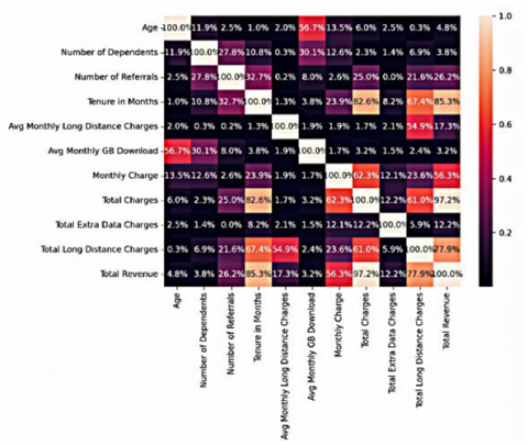
Similarly, the correlation method is used to remove the unnecessary numerical features from the dataset. The heat map is generated to determine which features are strongly correlated. The weakly correlated features are dropped from the dataset. Figure 1 presents the correlation heatmap of the dataset, highlighting relationships among customer demographics, service usage, and subscription details. Strong correlations provide insights for feature selection and predictive modeling.
Figure 1. Correlation heatmap
4.3 Handling null values
The dataset consists of null values in both categorical and numerical features [27]. These are handled using different methods, they are:
4.3.1 Categorical data
The null values in this field are handled using the statistical functions. Firstly, the unique values are determined for each field, and then their most repeated value among them is used to fill the null values. This is achieved through the mode () function and an Exploratory Data Analysis (EDA) technique called Fillna.
4.3.2 Numerical data
The null values in this field are handled using the KNN imputer module. Where the KNN stands for KNN, this method finds the value nearest to the data points and uses Euclidean distance to calculate the distance between the data points and the non-null values. It considers the KNNs and calculates the mean or median, respectively, to fill the null columns.
4.4 Encoding technique
Most of the machine learning models do not work with categorical data; it is necessary to encode them into numerical values. This is achieved through a one-hot encoding method where the categorical values are encoded into numerical data. Now this cleaned data is used for models to predict the churner.
4.5 Proposed model
Different classification models are applied to predict the churn classes. These classification models perform exceptionally well when they are used with ensemble techniques rather than using them individually. The dataset is split into training and testing samples. They are split in the ratio of 80:20, which means that 80% of the data is used for training the model, and the remaining 20% is used for testing the model. Both the dependent and independent features are split into train and test, respectively. The standardization technique is used to balance the scale of the features, because many machine learning models perform well when the data is scaled.
The standardized data is now used to train the model. The classification models used are a Random Forest classifier, which has an accuracy of 82% and Decision Tree classifier, which has an accuracy of 83%, and an SVM, which has an accuracy of about 81%. These models might perform well with a good accuracy score, but for a problem statement like customer churn prediction accuracy indicator does not tell us the exact performance of the model. Therefore, it is necessary to implement ensemble techniques. Here, bagging techniques like Random Forest classifier and boosting techniques like LightGBM are used to measure the performance.
The dataset consists of a lot of features. It is hard to identify which feature is more significant than the other. Though the correlation method and confusion matrix are used to reduce the dimensionality, there still exist features that do not participate in the prediction. It is necessary to ignore those less significant features. In order to overcome this, we have utilised the PCA method, which is well known for dimensionality reduction. This method uses the covariance matrix and identifies the features with greater variance, and utilizes the first few high variances for the prediction process. This not only increases the accuracy of the model but also accelerates the training time. When PCA is performed, the total number of features used for prediction is decreased from 27 to 16; only 16 features out of 27 had a major part in the prediction process.
This data is now bagged with various classification techniques to predict the churn rate of the customers. The most important factor here is that every algorithm has a unique set of parameters. It is difficult to select a parameter by the trial-and-error method, as it is not only time-consuming but also does not provide the correct combination of parameters. Hence, to resolve this issue, we use the RandomizedSearchCV method, which obtains the best parameter for training the model, and the cross-validation method is used to check for the accuracy. Once the hyperparameter tuning is done, the next step is to train the model using the training dataset. The accuracy of the Random Forest classifier was 79%, that of the Decision tree classifier was 75%, that of the SVM was 79%, and that of the LightGBM was 80.13%. But it is understood that accuracy does not play a major role in churn prediction. So the metric used to determine the performance is the AUC-ROC curve.
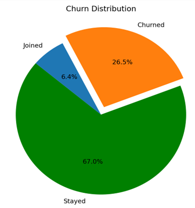
The dataset consists of imbalanced data where the positive and negative values are imbalanced. The dominant class is likely to be predicted by the models in this type of situation, whereas the minority class is completely ignored. Because of this imbalanced data, the performance metric accuracy is unable to accurately inform the prediction. For this reason, we utilize the AUC-ROC curve to assess the model's performance, taking into account recall and the F-measure with a confusion matrix to ascertain the genuine positive value. These metrics are used because the dependent column ‘Customer Status’ is a multiple-class feature. Where the positive rate is greater than the churn rate described in Figure 2. To handle this imbalanced data, the best model is LightGBM. The model prediction results are as follows: Random Forest has an AUC value of 0.82, Decision Tree has 0.85, SVM has 0.86, and LightGBM has 0.90. From the above performance metrics, it is observed that LightGBM has a greater value and is good at predicting the Churned customers [Class0] in our case.
Figure 2. Churn distribution
PCA was used to further reduce dimensionality after feature selection was completed using the Chi-Square test and correlation analysis to eliminate redundant and less important properties. By reducing multicollinearity among variables and increasing computational performance, PCA assisted in converting the chosen features into uncorrelated components. Hyperparameter tuning was conducted using a grid search with cross-validation, and the optimal parameters were chosen based on the best validation accuracy and AUC performance.
The experimental analysis shows us that the bagged model has shown better results than the one applied individually. Combining various models not only increases efficiency but also ensures that the classification of data is done accurately.
The LightGBM model performed exceptionally well and has an AUC of 0.9069. If the company is not ready to lose even a single customer, it's important to note the metrics like Recall, F1-Score, and Macro Average (which considers all the features equally).
Figure 3. AUC-ROC curve for Random Forest
The ROC curve for the Random Forest classifier shows a stronger upward bend toward the top-left corner, suggesting better classification performance than the Decision Tree. The model maintains consistently higher true-positive rates across a wide range of false-positive rates, which is supported by its higher AUC score. This indicates improved reliability in identifying churners. Figure 3 describes the AUC-ROC curve of the Random Forest classifier. It is understood from the curve that the class 0 (churn class) is classified for about 0.82%. The blue color line indicates that the variance in the data increases to a certain limit and then becomes stagnant towards the diagonal. The AUC values obtained from the models indicate that LightGBM outperformed other classifiers with an AUC of 0.906961. Minor discrepancies observed earlier (e.g., 0.90 vs. 0.906961) were due to rounding variations during summary presentation. consistent precision is maintained across all reported metrics. Furthermore, statistical significance and 95% confidence intervals were computed to confirm that the performance improvement of LightGBM over other models is statistically reliable. The confusion matrix analysis shows that most misclassifications occurred among borderline customers with moderate usage patterns. LightGBM achieved higher recall and precision, effectively minimizing false negatives. Its superior performance stems from gradient-based one-sided sampling (GOSS) and exclusive feature bundling, which enhance learning from imbalanced data and capture complex customer behavior more efficiently than other ensemble models.
The ROC curve for the Decision Tree model rises moderately above the diagonal reference line, showing limited separation between churn and non-churn classes. Although the curve approaches the upper-left region at certain thresholds, the overall shape indicates weaker discrimination capability compared to the ensemble models. This is reflected in its lower AUC value, indicating that the model has difficulty distinguishing borderline cases. Figure 4 describes the AUC-ROC curve of the Decision Tree classifier. It is understood from the curve that the class 0 (churn class) is classified for about 0.82%. The blue color line indicates that the variance in the data increases to a certain limit and then becomes stagnant towards the diagonal. From the comparison Random Forest model performs quite better when compared to the Decision Tree.
Figure 4. AUC-ROC curve for Decision Tree
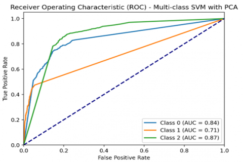
The SVM ROC curve demonstrates a smooth and pronounced arc toward the ideal top-left corner, showing solid discriminatory power. The higher AUC value reflects the model’s ability to separate churn and non-churn customers with reasonable accuracy, especially in mid-range threshold settings. Figure 5 describes the AUC-ROC curve of the SVM classifier. It is understood from the curve that the class 0 (churn class) is classified for about 0.84%. The blue color line indicates that the variance in the data increases to a certain limit and then becomes steep before the diagonal, and also for class 1 (joined class), the orange line is very steep, indicating that its classification is a false negative. From the comparison Random Forest model and the Decision Tree, the SVM performs poorly and does not classify the data properly.
Figure 5. AUC-ROC curve for SVM
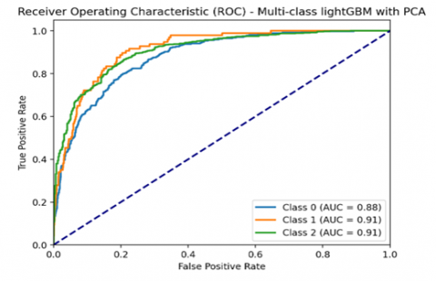
The LightGBM model exhibits the strongest ROC curve among all classifiers. The curve stays closest to the top-left corner, indicating high sensitivity even at low false-positive rates. The AUC of 0.9069 confirms superior overall performance and highly effective classification of churners. This curve shows that LightGBM captures the underlying data patterns more effectively than the other models. Figure 6 describes the AUC-ROC curve of the LightGBM classifier. It is understood from the curve that the class 0 (churn class) is classified for about 88%. The blue color line indicates that the variance in the data increases to a certain limit and then becomes stagnant towards the diagonal. From the comparison Random Forest model, the Decision Tree, and the SVM LightGBM classify the data more accurately and precisely.
Figure 6. AUC-ROC curve for LightGBM
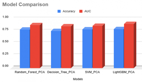
Table 1 describes the comparison of models with their accuracy and AUC value. These are bagged with PCA for dimensionality reduction. Among which LightGBM has an outstanding performance.
Table 1. Model comparison
|
Models |
Accuracy (%) |
AUC |
|
Random_Forest_PCA |
79.13 |
0.882031 |
|
Decision_Tree_PCA |
75.94 |
0.855050 |
|
SVM_PCA |
79.70 |
0.869104 |
|
Light_BGM_PCA |
80.13 |
0.906961 |
Figure 7 describes the comparison of various models along with their AUC values and accuracy. Describing that the LightGBM model performs well with an AUC of 0.9069.
Figure 7. Model comparison
The evaluation of the churn prediction models was carried out after reducing the feature space using PCA and training each algorithm within a bagging setup. Among the classifiers, LightGBM delivered the most consistent performance, achieving an accuracy of 80.13% and an AUC of 0.9069, with SVM, Random Forest, and Decision Tree following behind. These outcomes suggest that combining PCA with ensemble learners helps the models handle the telecom dataset more efficiently and with greater stability.
Analysis of the confusion matrices showed that errors mainly occurred for customers whose behavior fell between clear churn and non-churn categories. LightGBM demonstrated stronger recall for the churn class, which is valuable in practical settings because correctly identifying potential churners enables earlier interventions.
It should be noted that all models were tested only after PCA and bagging were applied. The purpose of this research was to observe how these techniques function together when dealing with imbalanced data, not to compare them against versions without PCA or bagging. Therefore, no superiority claims are made; rather, the results reflect the effectiveness of the selected approach within the defined experimental scope.
The proposed PCA-enabled ensemble framework demonstrates that telecom churn can be modeled effectively using structured customer data, offering practical support for early retention decisions. Beyond the numerical results, the work highlights how dimensionality reduction and bagging can help stabilize model performance when dealing with imbalanced customer records—an issue common in real-world telecom environments. However, the study is limited by its reliance on static, tabular customer features and the absence of comparisons with non-PCA or non-bagged configurations. Future research can expand the framework by incorporating temporal usage trends, customer satisfaction surveys, and network-level behavior. Deploying the model in a real-time churn monitoring pipeline and exploring deep learning approaches—such as LSTM networks for sequential behavioral patterns—would further strengthen the system’s predictive capability and practical applicability. Main Contributions: Implementation of a hybrid PCA–bagging framework that enhances model stability and performance on imbalanced telecom datasets. Comparative evaluation of multiple ensemble classifiers to identify the most effective churn prediction model. Integration of dimensionality reduction with ensemble learning to optimize computational efficiency without compromising accuracy.
Future research can focus on incorporating customer satisfaction surveys and behavioral feedback to strengthen model interpretability, deploying the system in a real-time churn monitoring environment, and extending the approach with deep learning architectures such as LSTM networks to capture time-dependent customer behavior.
[1] Azzam, D., Hamed, M., Kasiem, N., Eid, Y., Medhat, W. (2023). Customer churn prediction using Apriori algorithm and ensemble learning. In 2023 5th Novel Intelligent and Leading Emerging Sciences Conference (NILES), Giza, Egypt, pp. 377-381. https://doi.org/10.1109/NILES59815.2023.10296608
[2] Mitkees, I.M., Badr, S.M., ElSeddawy, A.I.B. (2017). Customer churn prediction model using data mining techniques. In 2017 13th International Computer Engineering Conference (ICENCO), Cairo, Egypt, pp. 262-268. https://doi.org/10.1109/ICENCO.2017.8289798
[3] Nababan, A.A., Sutarman, Zarlis, M., Nababan, E.B. (2024). Multiclass logistic regression classification with PCA for imbalanced medical datasets. Mathematical Modelling of Engineering Problems, 11(9): 2377-2387. https://doi.org/10.18280/mmep.110911
[4] Wu, S., Yau, W.C., Ong, T.S., Chong, S.C. (2021). Integrated churn prediction and customer segmentation framework for telco business. IEEE Access, 9: 62118-62136. https://doi.org/10.1109/ACCESS.2021.3073776
[5] Mishra, A., Reddy, U.S. (2017). A comparative study of customer churn prediction in telecom industry using ensemble based classifiers. In Proceedings of the 2017 International Conference on Inventive Computing and Informatics (ICICI), Coimbatore, India, pp. 721-725. https://doi.org/10.1109/ICICI.2017.8365230
[6] Alotaibi, M.Z., Haq, M.A. (2024). Customer churn prediction for telecommunication companies using machine learning and ensemble methods. ETASR – Engineering, Technology & Applied Science Research, 14(2): 7480-7492. https://doi.org/10.48084/etasr.7480
[7] Kanwal, S., Rashid, J., Kim, J., Nisar, M.W., Hussain, A., Batool, S., Kanwal, R. (2021). An attribute weight estimation using particle swarm optimization and machine learning approaches for customer churn prediction. In Proceedings of the 2021 International Conference on Innovative Computing (ICIC), pp. 745-750. https://doi.org/10.1109/icic53490.2021.9693040
[8] Saha, S., Saha, C., Haque, M.M. (2024). ChurnNet: Deep learning enhanced customer churn prediction in telecommunication industry. IEEE Access, 12: 4471-4482. https://doi.org/10.1109/ACCESS.2024.3349950
[9] Srinivasan, R., Rajeswari, D., Elangovan, G. (2023). Customer churn prediction using machine learning approaches. In 2023 International Conference on Artificial Intelligence and Knowledge Discovery in Concurrent Engineering (ICECONF), Chennai, India, pp. 1-6. https://doi.org/10.1109/ICECONF57129.2023.10083813
[10] Ahmed, A., Linen, D.M. (2017). A review and analysis of churn prediction methods for customer retention in telecom industries. In 2017 4th International Conference on Advanced Computing and Communication Systems (ICACCS), Coimbatore, India, pp. 1-7. https://doi.org/10.1109/ICACCS.2017.8014605
[11] Ullah, I., Raza, B., Malik, A.K. (2019). A churn prediction model using random forest: Analysis of machine learning techniques for churn prediction and factor identification in telecom sector. IEEE Access, 7: 60134-60149. https://doi.org/10.1109/ACCESS.2019.2914999
[12] Bharambe, Y., Deshmukh, P., Karanjawane, P., Chaudhari, D., Ranjan, N.M. (2023). Churn prediction in telecommunication industry. In 2023 International Conference for Advancement in Technology (ICONAT), Goa, India, pp. 1-5. https://doi.org/10.1109/ICONAT57137.2023.10080425
[13] Siddika, A., Faruque, A., Masum, A.K.M. (2021). Comparative analysis of churn predictive models and factor identification in telecom industry. In 2021 24th International Conference on Computer and Information Technology (ICCIT), Dhaka, Bangladesh, pp. 1-6. https://doi.org/10.1109/ICCIT54785.2021.9689881
[14] Dev, D.R., Biradar, V.S., Chandrasekhar, V., Sahni, V., Kulkarni, P., Negi, P. (2024). Uncertainty determination and reduction through novel approach for industrial IoT. Measurement: Sensors, 31: 100995. https://doi.org/10.1016/j.measen.2023.100995
[15] Bogaert, M., Delaere, L. (2023). Ensemble methods in customer churn prediction: A comparative analysis of the state-of-the-art. Mathematics, 11(5): 1137. https://doi.org/10.3390/math11051137
[16] Zhu, B., Qian, C., Vanden Broucke, S., Xiao, J., Li, Y. (2023). A bagging-based selective ensemble model for churn prediction on imbalanced data. Expert Systems with Applications, 227: 120223. https://doi.org/10.1016/j.eswa.2023.120223
[17] Chang, V., Hall, K., Xu, Q.A., Amao, F.O., Ganatra, M.A., Benson, V. (2024). Prediction of customer churn behavior in the telecommunication industry using machine learning models. Algorithms, 17(6): 231. https://doi.org/10.3390/a17060231
[18] Mirabdolbaghi, S.M.S., Amiri, B., Pan, W.T. (2022). Model optimization analysis of customer churn prediction using machine learning algorithms with focus on feature reductions. Discrete Dynamics in Nature and Society, 2022: 5134356. https://doi.org/10.1155/2022/5134356
[19] Sikri, A., Jameel, R., Idrees, S.M., Kaur, H. (2024). Enhancing customer retention in telecom industry with machine learning driven churn prediction. Scientific Reports, 14: 13097. https://doi.org/10.1038/s41598-024-63750-0
[20] Peng, K., Peng, Y. (2022). Research on telecom customer churn prediction based on GA-XGBoost and SHAP. Journal of Computer and Communications, 10: 107-120. https://doi.org/10.4236/jcc.2022.1011008
[21] Noviandy, T.R., Idroes, G.M., Hardi, I., Afjal, M., Ray, S. (2024). A model-agnostic interpretability approach to predicting customer churn in the telecommunications industry. Infolitika Journal of Data Science, 2(1): 34-44. https://doi.org/10.60084/ijds.v2i1.199
[22] Omar, I., Saleh, A.A.M. (2023). A comprehensive review of design and operational parameters influencing airlift pump performance. Mathematical Modelling of Engineering Problems, 10(3): 1063-1073. https://doi.org/10.18280/mmep.100342
[23] Barsotti, A., Gianini, G., Mio, C., Lin, J., Babbar, H., Singh, A., Damiani, E. (2024). A decade of churn prediction techniques in the telco domain: A survey. SN Computer Science, 5(4): 404. https://doi.org/10.1007/s42979-024-02722-7
[24] Seid, M.H., Woldeyohannis, M.M. (2022). Customer churn prediction using machine learning: Commercial bank of Ethiopia. In 2022 International Conference on Information and Communication Technology for Development for Africa (ICT4DA), Bahir Dar, Ethiopia, pp. 1-6. https://doi.org/10.1109/ICT4DA56482.2022.9971224
[25] Thanam, A., Malchijah Raj, M.S., Joel, M.R., Shanthakumar, P., Jacson, J.J. (2024). Enhancing telecom customer loyalty through churn prediction models. In 2024 8th International Conference on Electronics, Communication and Aerospace Technology (ICECA), Coimbatore, India, pp. 770-774. https://doi.org/10.1109/ICECA63461.2024.10800923
[26] Mandić, M., Kraljević, G. (2022). Churn prediction model improvement using automated machine learning with social network parameters. Revue d'Intelligence Artificielle, 36(3): 373-379. https://doi.org/10.18280/ria.360304
[27] Adeleke, A.A., Oki, M., Anyim, I.K., Ikubanni, P.P., Adediran, A.A., Balogun, A.A., Orhadahwe, T.A., Omoniyi, P.O., Olabisi, A.S., Akinlabi, E.T. (2022). Recent development in casting technology: A pragmatic review. Revue des Composites et des Matériaux Avancés-Journal of Composite and Advanced Materials, 32(2): 91-102. https://doi.org/10.18280/rcma.320206