Purba Daru Kusuma*![]() | Tito Waluyo Purboyo
| Tito Waluyo Purboyo![]()
© 2025 The authors. This article is published by IIETA and is licensed under the CC BY 4.0 license (http://creativecommons.org/licenses/by/4.0/).
OPEN ACCESS
Over the last ten years, many novel metaheuristic strategies have emerged but most of them are metaphor-inspired algorithms. In this study, we introduce a newly developed metaphor-free method named the push spread algorithm (PSA). Term push represents exploitation while spread represents exploration. It accommodates six actions and four references including the biggest agent, the bigger agents, the smaller agents, and the boundaries. The effectiveness of PSA is investigated through two cases including 23 standard functions and 2 economic load dispatch (ELD) problems. The performance of PSA was evaluated against five other optimization strategies: the farmer and season approach (FSA), coati optimizer (COA), osprey optimizer (OOA), kookaburra optimizer (KOA), and particle swarm optimization (PSO). The result shows that PSA is better than FSA, COA, OOA, KOA, and PSO in 21, 12, 10, 12, and 23 functions. Meanwhile, PSA is in the third best in handling the first ELD case and in the fourth best in handling the second one. This result makes PSA acceptable as a stochastic optimization to achieve quasi-optimal solution. Findings indicate that PSA demonstrates strong capability for tackling large-scale functions and remains effective when applied to fixed-size problems and ELD tasks.
stochastic optimization, metaphor-free metaheuristic, power system scheduling, economic load dispatch, swarm intelligence
Cost becomes the most important issue in many studies related to the operational of various systems. Cost becomes the rationale consequence of the operation of any system. This cost can come from fuel or energy consumption [1], labor utilization [2], maintenance [3], emission handling [4], waste [5], time or opportunity lost [6], and so on. Management must focus on keeping this cost as low as possible for the continuity of the operation of the system as this cost becomes the main factor in the selling price. Keeping the cost low gives positive impact to make the price still acceptable and competitive. That is why minimizing cost has become the most famous goal in many optimization studies. This goal in minimizing cost can be found in many optimization studies in various fields, such as manufacturing [7], transportation [8], logistics [9], and power systems [10].
A well-known challenge in power system optimization is the economic load dispatch (ELD). This task involves determining the optimal allocation of generation levels for each unit in the network [11]. This cumulative power must be equal to the required demand which in general is known in advance. Each generator has its own operational range. The main or general goal of ELD problem is minimizing the total operational cost where each generator has its own cost structure. In addition, numerous aspects are taken into account when dealing with the ELD issue, including factors like the valve-point effect [12], restrictions due to ramping limits [13], forbidden operating zones [14], among others. On the other hand, each power system has its own mixture of generators where in some studies, the power system consists of generators from various energy resources, such as fossils, wind, water, nuclear, and so on. In many ELD studies, metaheuristic algorithm is often used as the optimization tool.
Many metaheuristics-algorithms that have been introduced in this recent decade are metaphor-inspired algorithms and developed root in swarm intelligence (SI) framework. The inspiration behind many metaheuristic techniques is often drawn from natural occurrences, especially the survival strategies of animals in reproduction and foraging activities. Several methods developed from this concept include the coati optimization algorithm (COA) [15], kookaburra optimization algorithm (KOA) [16], osprey optimization algorithm (OOA) [17], komodo mlipir algorithm (KMA) [18], golden jackal optimization (GJO) [19], fennec fox optimization (FFO) [20], fossa optimization algorithm (FOA) [21], salamander optimization algorithm (SOA) [22], among others. Several optimization paradigms have drawn inspiration from socio–cultural or human-centered dynamics, including the farmer–season framework (FSA) [23], motorbike courier-based optimization (MCO) [24], an enhanced variant of the social force method (MSFA) [25], the physician–patient model (DPO) [26], the deep sleep mechanism (DSO) [27], and the program manager-based approach (PMOA) [28], among others. In contrast, other studies emphasize approaches detached from metaphorical analogies, such as the fully informed search method (FISA) [29], subtraction–average optimization (SABO) [30], average–subtraction optimization (ASBO) [31], the adaptive grouping algorithm (AGA) [32], and golden search optimization (GSO) [33], among several additional proposals.
The rapid emergence of various new methods has been driven by multiple factors. One major factor is the absence of a single metaheuristic technique that consistently outperforms others across every type of optimization challenge. The second aspect is that there are numerous mathematical techniques that can be explored to create a new algorithm and there are numerous methods to implement these techniques. In addition to designing novel algorithms, researchers have often relied on mathematical approaches to refine or adjust existing metaheuristic methods. Such enhancements are evident in well-established techniques like the genetic algorithm (GA), particle swarm optimization (PSO), and various others. Another important point is the abundance of real-world optimization challenges across diverse domains, especially in engineering, which provide valuable testbeds for evaluating newly developed algorithms.
Although numerous advanced metaheuristic techniques have been introduced, this study puts forward a novel approach known as the push spread algorithm (PSA). This algorithm is metaphor-free so that it becomes the alternative for the many metaphor-inspired algorithms. There is critique regarding the metaphor-inspired algorithms as many of them hide their trivial novel mechanics by utilizing the metaphor to cover it. PSA is established root in SI framework so that it is a population-based technique where individuals become autonomous agents that act collectively but without any central command. Related to its name, PSA lays its effort on push and spread actions. The push action represents exploitation as the agent moves toward the entities that give higher probability for improvement. Contrary, the spread action represents the exploration where agent moves away from the convergence to find alternatives to avoid being trapped within the local optimal region.
Due to the goal and the unresolved problems which are previously explained, the following points highlight the scholarly value produced through this study.
The rest of this article is organized in the following way: Section 2 outlines and synthesizes recent research related to ED, while Section 3 introduces the proposed PSA, detailing its underlying idea, computational procedure, and mathematical framework. Section 4 presents the experiment that is conducted to investigate the effectiveness and competitiveness of PSA including the following results. Section 5 provides discussion related to the experiment result, findings, and limitations. Section 6 provides an overview of the key findings and outlines potential directions for upcoming research.
There are numerous studies in ED problems. Despites in general or standard form, ED problem also has derivatives, such as ELD problem [34], unit commitment (UC) problem [35], economic emission dispatch (EED) problem [36], optimal power flow (OPF) problem [37], and so on. Below is the example of some recent studies in the ED problem.
Hassan et al. [12] employ eagle-strategy supply-demand algorithm with chaotic (ESCSDO). ESCSDO is the modification of the existing supply demand optimization (SDO), which is an algorithm that was developed root in economic concept or principle. Hassan et al. [12] introduced an approach known as the eagle strategy, designed to guide the population closer to optimal candidates while steering it away from poor ones. Moreover, as the name suggests, ten chaotic maps are introduced to make the convergence process better. In their work, the suggested ESCSDO was confronted with several algorithms, such as the GA, SDO, and PSO.
Spea [38] suggested the enhanced version of manta ray foraging optimization (MRFO) in his ED study. There are four variants related to this enhancement. The first derivative is opposition-based MRFO. The second type is quasi-oppositional MRFO (QMRFO). The third extension of MRFO is formulated using an opposition-driven generation-jumping strategy (JOMRFO). The fourth version applies to a quasi-oppositional approach combined with JQMRFO. This enhancement originates from three core principles: opposition-based learning, quasi-oppositional learning, and the jumping rate mechanism. Opposition-based learning is a mechanism for exploration within the solution space by implementing the opposite numbers or points. Meanwhile, quasi-oppositional learning is the variant of opposition-based learning by converting the standard version of opposition-based learning which is deterministic into stochastic so that the opposite number within space is not static. In the generation jumping, oppositional action is conducted root in the stochastic parameter called probabilistic jumping rate. If a generated random number between 0 and 1 is less than this jumping rate, then the oppositional action is taken whether it is oppositional learning or quasi-oppositional learning. Otherwise, the oppositional action is not taken so that the solution stays in its current location. Overall, this improvement is designed to avoid the local optimal.
Nagarajan et al. [39] introduced a refined variant of the cheetah optimization method, termed the Enhanced Cheetah Optimizer Algorithm (ECOA), designed to address the economic dispatch (ED) problem. The improvement of the CO was conducted through several mechanisms. The normal distribution for the step size during the searching strategy is replaced by the sine map. Still during the searching strategy, the factor that is controlled by the iteration is replaced by using the gap between the agent and the selected agent. Meanwhile, during the attacking strategy, the normal distribution is replaced with the Levy flight. In this work, the suggested ECOA is confronted with several algorithms, such as the improved version of PSO, grey wolf optimization, and the standard form of CO.
Hassan et al. [40] suggested the improved version of white shark optimization (WSO) called leader white shark optimization (LWSO) to solve the ELD problems. This improvement is also designed to avoid the local optimal. The improvement is conducted root in the mechanism called leader-based mutation selection. In the classic WSO, there are two best solutions that are used as references, including the global best and the local best. Conversely, in LWSO, the references are the best solution, the second-best solution, and the third best solution. This leader-based solution is generated after the agent moves using the standard WSO. Then, this leader-based solution is used to replace the location of the agent after conducting searches, only if this leader-based solution is better than the previous ones. In this work, the LWSO is confronted with the standard WSO, northern goshawk optimization (NGO), GJO, and so on.
Tariq et al. [41] introduced the Directional Bat Algorithm (DBA) as an enhanced variant of the traditional Bat Algorithm (BA) for addressing ELD tasks. Unlike DBA, the conventional BA typically produces candidate solutions by performing a stochastic walk in the neighborhood of the current best candidate. When the random walk process does not yield progress, one candidate is chosen at random from the population and evaluated against the newly generated candidate. Whichever of the two performs better will replace the current solution. In the context of the DBA, an agent may follow two possible routes: moving closer to the global best solution or carrying out a localized exploration. In this study, the DBA approach is assessed in comparison with three alternative methods, namely the baseline DBA, PSO, and GA.
Secui et al. [42] introduced an enhanced variant of the social group optimization (SCO) technique, referred to as chaotic social group optimization (CSCO), to address the ELD problem. The refinement was accomplished through the incorporation of five different chaotic mapping strategies into the conventional SCO framework. These maps include double, logistic, iterative, singer, and cat. In general, the procedure of CSCO is the same as the standard CSCO. But, in CSCO, these logistic maps are used to replace the random numbers that are used during the initialization, improving stage, and acquiring phase. In its standard form of SCO, the random numbers follow uniform distribution. In this work, the CSCO was confronted with many algorithms, such as Jaya algorithm, PSO, GA, and TSA.
In general, several use cases are used in every study. Many of these studies used common cases or systems. Singh et al. [43] evaluated their approach on three scenarios, namely networks with 6, 13, and 15 generating units. In contrast, Secui et al. [42] carried out experiments on five configurations consisting of systems with 10, 20, 30, 40, and 50 units. Zein et al. [14] examined three alternatives corresponding to 10-, 13-, and 40-unit arrangements. Meanwhile, Hassan et al. [12] investigated four different test systems that involved 6, 13, 15, and 40 units.
Many ED studies also employed their own considerations or additional parameters. Hassan et al. [12] incorporate the influence of valve-point loading into the formulation of the cost objective. In addition, restrictions such as ramp-rate constraints and prohibited zones are applied, which compress the feasible operating region compared to the theoretical case. The ramp rate limit is introduced to avoid the power of generator jumping too high or falling too low in the next time frame. The prohibited operating zone is introduced because of the vibration on the shaft bearing. This VPLE aspect is also considered in Zein’s work [14]. Power loss is considered in the studies by Hassan et al. [12] so that the output must equal the summation of the demand and power loss. In the study by Tariq et al. [41] the thermal generators are combined with the solar and wind powered generators, where the cost function does not follow the quadratic equation. In the wind and solar power generators, the cost comes from operation and maintenance. Puspitasari et al. [13] formulated the objective function by merging fuel expenses with emission-related costs, thereby transforming the ED task into what is known as the EED problem.
This short review shows that there are numerous variations in ED studies. These variations may come from several aspects, including cases, considerations, and the optimization tools. As mentioned previously, most of these studies used existing metaheuristic algorithms, particularly in their improvised form. On the other hand, only a few studies investigate ED problems but also introduce a new metaheuristic algorithm in single paper. Root in this circumstance, this study proposes a new metaheuristic algorithm and using ED problems as cases despites the standard functions.
3.1 Suggested PSA model
This suggested PSA is established as a metaphor-free technique. Root in its name, there are two key terms which are push and spread. Push represents exploitation while spread represents exploration. Within SI, PSA functions as a foundational method where multiple agents collaborate collectively, resembling a swarm, to carry out a guided exploration. PSA is also established as a multiple-search technique. PSA accommodates multiple references including the biggest agent, the bigger agents, the smaller agents, and the boundary. The passage toward the biggest agent and the bigger agents represents exploitation. Conversely, the passage avoiding the smaller agents and toward the boundary represents exploration.
There are six actions that can be conducted by each agent. These actions are accommodated into two stages in every iteration during the initial phase, the agent is allowed to choose among three possible operations: the first, the second, or the third. In the following phase, the available options shift, and the agent can instead select from the fourth, fifth, or sixth operation. The probability of becoming the picked action is equal among three actions.
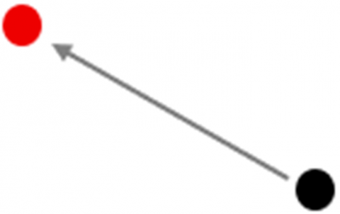
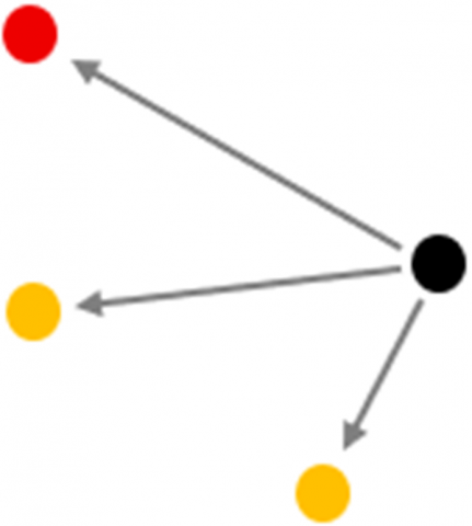
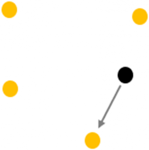
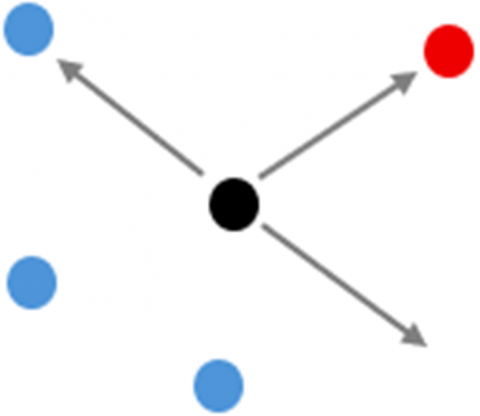
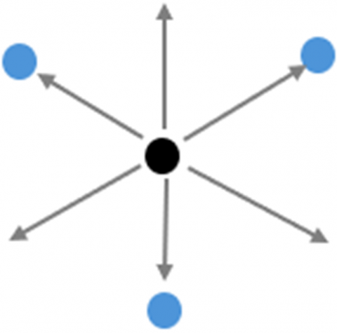
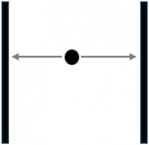
Details and sequence of these six actions are provided below: (1) The initial movement is directed solely toward the dominant or biggest agent. (2) Subsequently, the process evolves into gradual advancements encompassing all relatively bigger agents, including the biggest one. (3) In the third stage, the orientation is selectively targeted toward a single agent chosen from the collective of bigger agents together with the biggest agent. (4) The fourth stage represents a composite mechanism, either combining progression toward both the biggest agent and a selected agent or integrating advancement toward the biggest agent with simultaneous avoidance of the selected agent. (5) Finally, the fifth stage involves incremental advancement toward all bigger agents while explicitly excluding interactions with smaller agents. (6) The sixth action is the passage toward the upper boundary or lower boundary.
|
(a) |
(b) |
(c) |
|
(d) |
(e) |
(f) |
Figure 1. Illustration of six actions in PSA
The visualization of these actions is provided in Figure 1. The black dot represents the agent. The red dot represents the biggest agent. The yellow dots represent the bigger agent. The blue dots represent the other agents. The black bars represent the boundaries.
Algorithm 1 together with Eqs. (1)-(23) describe the structured representation of PSA. While the algorithmic steps are outlined in the form of pseudocode, the mathematical operations underlying the procedure are expressed in Eqs. (1)-(23).
$X=\left\{x_1, x_2, \ldots, x_n\right\}$ (1)
$x_i=\left\{x_{i, 1}, x_{i, 2}, x_{i, 3}, \ldots, x_{i, m}\right\}$ (2)
Eq. (1) and Eq. (2) formalize the establishment of the swarm. Eq. (1) defines the establishment of the swarm that consists of certain number of agents. Eq. (2) defines the establishment of each agent that contains certain number of values where each value represents the position in a dimension.
$x_{i, j}=b_{l o w, j}+r_1\left(b_{u p, j}-b_{l o w, j}\right)$ (3)
$x_{b g t}^{\prime}=\left\{\begin{aligned} x_i, \min \left(f\left(x_i\right), f\left(x_{b g t}\right)\right) & =f\left(x_i\right) \\ x_{b g t}, \min \left(f\left(x_i\right), f\left(x_{b g t}\right)\right) & =f\left(x_{b g t}\right)\end{aligned}\right.$ (4)
Eq. (3) and Eq. (4) formalize the processes in the initialization phase. Eq. (3) defines the initial solution or value of the agent is uniformly located in the solution space. Then, Eq. (4) is used for the update of the biggest agent root in the value of the agent. The updating process of the biggest agent also occurs at every stage during the iteration.
$a_{1, i, j}=x_{i, j}+r_1\left(x_{bg t, j}-2 x_{i, j}\right)$ (5)
$P_i=\left\{\forall x_k \in X \mid \min \left(f\left(x_k\right), f\left(x_i\right)\right)=f\left(x_k\right)\right\} \cup x_{b g t}$ (6)
$a_{2, i, j}=x_{i, j}+\frac{\sum_{k=1}^{n\left(P_i\right)} r_1\left(p_{i, k, j}-2 x_{i, j}\right)}{n\left(P_i\right)}$ (7)
$x_{s e l 1, i}=r_2\left(P_i\right)$ (8)
$a_{3, i, j}=x_{i, j}+r_1\left(x_{s e l, i, j}-2 x_{i, j}\right)$ (9)
$x_{\text {sel} 2, i}=r_2(X)$ (10)
$a_{s 1, i, j}=r_3\left(x_{b g t, j}-2 x_{i, j}\right)$ (11)
$a_{s 2, i, j}=r_3\left(x_{s e l 2, i, j}-2 x_{i, j}\right)$ (12)
$a_{s 3, i, j}=r_3\left(x_{i, j}-x_{s e l 2, i, j}\right)$ (13)
$\begin{aligned} & a_{4, i, j} =\left\{\begin{array}{c}x_{i, j}+a_{s 1 . i . j}+a_{s 2, i, j}, \min \left(f\left(x_i\right), f\left(x_{s e l 2}\right)\right)=f\left(x_{s e l 2}\right) \\ x_{i, j}+a_{s 1 . i . j}+a_{s 3, i, j}, \min \left(f\left(x_i\right), f\left(x_{s e l 2}\right)\right)=f\left(x_i\right)\end{array}\right.\end{aligned}$ (14)
$W_i=\left\{\forall x_k \in X \mid \min \left(f\left(x_k\right), f\left(x_i\right)\right)=f\left(x_i\right)\right\}$ (15)
$a_{s 4, i, j}=\sum_{k=1}^{n\left(P_i\right)} r_1\left(p_{i, k, j}-2 x_{i, j}\right)$ (16)
$a_{s 5, i, j}=\sum_{k=1}^{n\left(w_i\right)} r_1\left(x_{i, j}-w_{i, k, j}\right)$ (17)
$a_{5, i, j}=x_{i, j}+\frac{a_{s 4, i, j}+a_{s 5, i, j}}{n(X)}$ (18)
$a_{6, i, j}=\left\{\begin{array}{l}x_{i, j}+r_1\left(b_{u p, j}-x_{i, j}\right), r_1<0.5 \\ x_{i, j}+r_1\left(x_{i, j}-b_{l o w, j}\right), r_1 \geq 0.5\end{array}\right.$ (19)
Eqs. (5)-(19) describe the framework of six possible operations available to every agent. Specifically, Eq. (5) introduces the initial operation, while Eq. (6) specifies the creation of a pool that gathers all larger agents together with the single largest one. Eq. (7) defines the second action. Eq. (8) defines the random selection of an agent from the pond containing bigger agents. Eq. (9) defines the third action. Eq. (10) defines the random selection of an agent from the swarm. Eqs. (11)-(13) specify three components of the fourth operation, namely moving in the direction of the biggest agent, advancing toward the selected agent, and shifting away from the selected agent. Eq. (14) defines the fourth action. Eq. (15) defines the establishment of the pond containing all smaller agents. Eq. (16) and Eq. (17) defines the two parts that are used in the fifth action, which are the passage toward all bigger agents and the passage avoiding all smaller agents. Eq. (18) defines the fifth action. Eq. (19) defines the sixth action.
$c_{1, i}=\left\{\begin{array}{c}a_{1, i}, r_1 \leq 0.33 \\ a_{2, i}, 0.33<r_1 \leq 0.67 \\ a_{3, i}, r_1>0.67\end{array}\right.$ (20)
$x_i^{\prime}=\left\{\begin{array}{c}c_{1, i}, \min \left(f\left(c_{1, i}\right), f\left(x_i\right)\right)=f\left(c_{1, i}\right) \\ x_i, \min \left(f\left(c_{1, i}\right), f\left(x_i\right)\right)=f\left(x_i\right)\end{array}\right.$ (21)
$c_{2, i}=\left\{\begin{array}{c}a_{4, i}, r_1 \leq 0.33 \\ a_{5, i}, 0.33<r_1 \leq 0.67 \\ a_{6, i}, r_1>0.67\end{array}\right.$ (22)
$x_i^{\prime}=\left\{\begin{array}{c}c_{2, i}, \min \left(f\left(c_{2, i}\right), f\left(x_i\right)\right)=f\left(c_{2, i}\right) \\ x_i, \min \left(f\left(c_{2, i}\right), f\left(x_i\right)\right)=f\left(x_i\right)\end{array}\right.$ (23)
|
Algorithm 1. Push spread algorithm |
|
|
1 |
start |
|
2 |
for i=1 to n(X) |
|
3 |
initialize xi using Eq. (3) |
|
4 |
update xbgt using Eq. (4) |
|
5 |
stop for |
|
6 |
for t=1 to T |
|
7 |
for i=1 to n(X) |
|
8 |
generate c1,i using Eq. (20) |
|
9 |
update xi using Eq. (21) and xbgt using Eq. (4) |
|
10 |
generate c1,i using Eq. (22) |
|
11 |
update xi using Eq. (23) and xbgt using Eq. (4) |
|
12 |
stop for |
|
13 |
stop for |
|
14 |
return xbgt |
|
15 |
stop |
Eqs. (20)-(23) define the establishment of the first and second candidates, including the update of the agent root in these candidates. Eq. (20) defines the establishment of the first solution candidate root in the first, second, or third. Eq. (21) defines the update of the agent root in the first candidate representing the first stage. Eq. (22) defines the establishment of the second solution candidate root in the fourth, fifth, or sixth action. Eq. (23) defines the update of the agent root in the second candidate representing the second stage.
The pseudocode of PSA is presented in Algorithm 1. Lines 2–5 describe the setup phase, while lines 6–13 outline the repetitive process. The outcome is the optimal solution obtained. In Algorithm 1, the initialization stage involves cycling through the entire swarm. During the iteration phase, two nested loops are present: the outer one continues until the maximum number of iterations is reached, and the inner one goes through all swarm members as each individual performs its search activity.
There are two more loops in every stage. During the initial iteration, the system attempts to identify every participant in the swarm to establish a pool. However, this detection is not assured, since in the opening stage the chance of it occurring is roughly 67%, while in the following stage the likelihood decreases to about 33%. Then, there is an additional loop in every searching process that runs for whole dimension. Root in this explanation, the complexity during the initialization is presented as O(nd) while the complexity during the iteration is presented as O(n2dT).
3.2 Model of the ELD problem
This work employs the standard ELD problem. In general, the goal is minimizing the total fuel cost or operation cost where the cost function of each generator is presented in quadratic function. Then, there are two constraints. The restriction on inequality ensures that every generator operates only within its designated power limits. In contrast, the equality condition requires that the overall generated power exactly matches the predetermined demand. The conventional formulation of the ELD problem is expressed mathematically in Eqs. (24)-(29).
$o_{E L D}=\min \left(e_{t o t}\right)$ (24)
$e_{t o t}=\sum_{n(G)} e\left(g_j\right)$ (25)
$e\left(g_j\right)=s_{1, j} g_j^2+s_{2, j} g_j+s_{3, j}$ (26)
$g_{\text {tot }}=g_{\text {demand }}$ (27)
$g_{t o t}=\sum_{n(G)} g_j$ (28)
$g_{\min , j} \leq g_j \leq g_{\max , j}$ (29)
The discussion that follows covers Eqs. (24)-(29). In Eq. (24), the main objective is expressed as reducing the overall expenditure. Meanwhile, Eq. (25) specifies that the sum of expenses from every generator constitutes this total cost. Eq. (26) defines the quadratic function as the cost function of each generator. Eq. (27) defines the equality constraint. Eq. (28) defines the accumulation of power from all generators to create the total power. Eq. (29) defines the inequality constraint.
The effectiveness of PSA is investigated through its implementation to solve optimization problems. In this paper, the theoretical problems are represented by the 23 standard functions while the practical problems are represented by two cases of ELD problem. In this investigation, PSA is compared with five other metaheuristic algorithms, including FSA [23], COA [15], OOA [17], KOA [16], and PSO [44]. Throughout the experiment, each method was executed with a group consisting of five agents and was allowed to progress for up to twenty iterations. This setting is applied in both standard functions and ELD problems.
In both cases, the swarm size is 5 while the maximum iteration is 20. This setting is designed to investigate the performance of the algorithms to achieve optimal or quasi-optimal results in the limited computational environment. Despite the concern of producing the convergence too soon, achieving fast optimal solution is still needed.
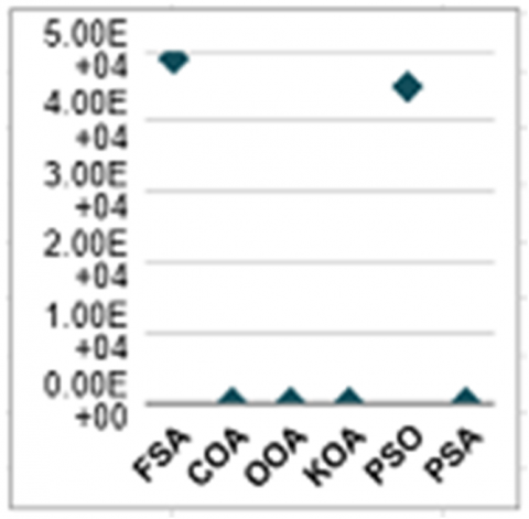
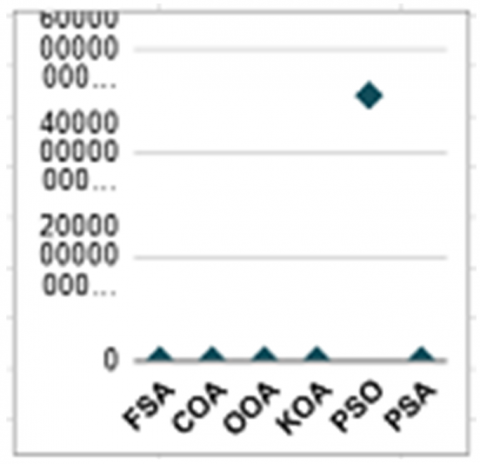
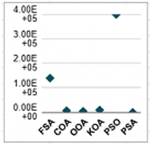
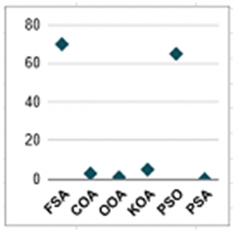
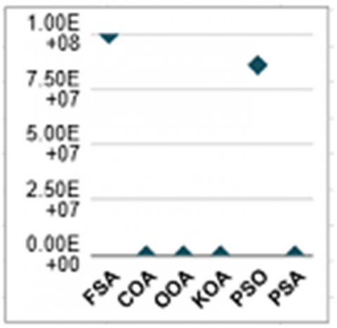
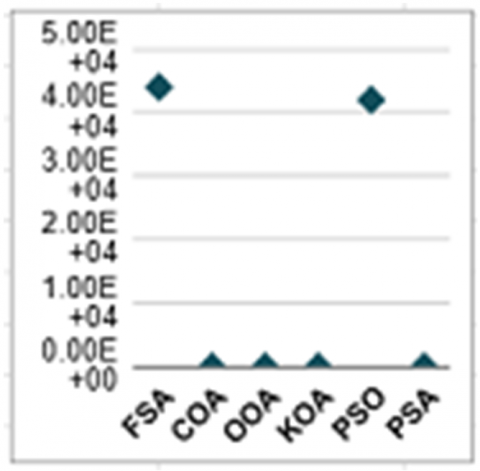
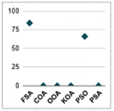
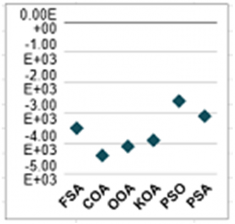
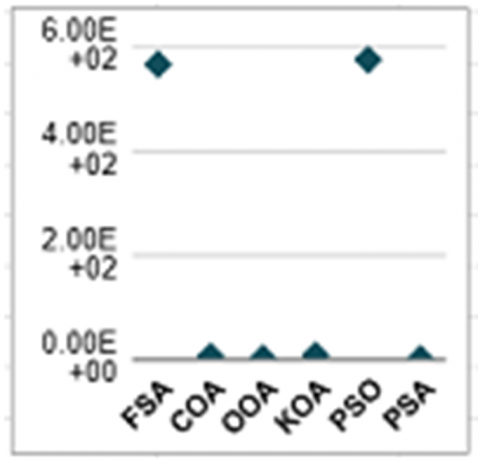
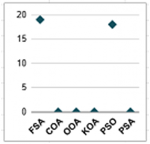
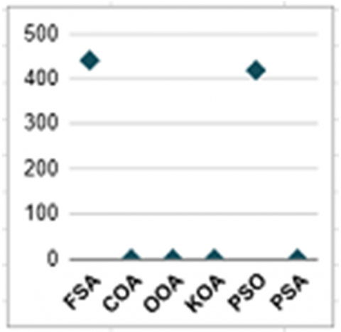
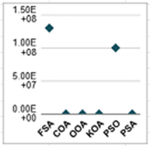
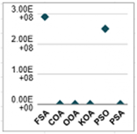
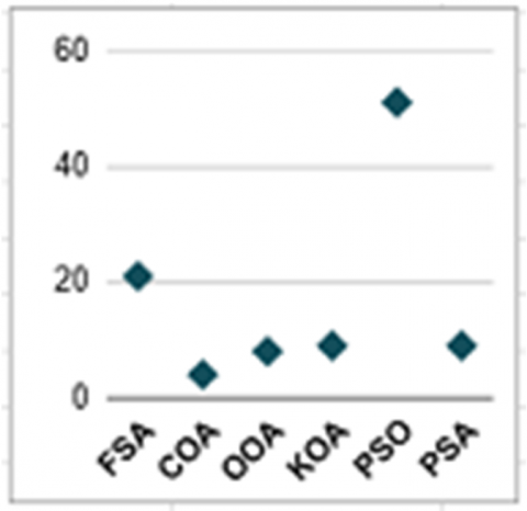
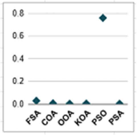
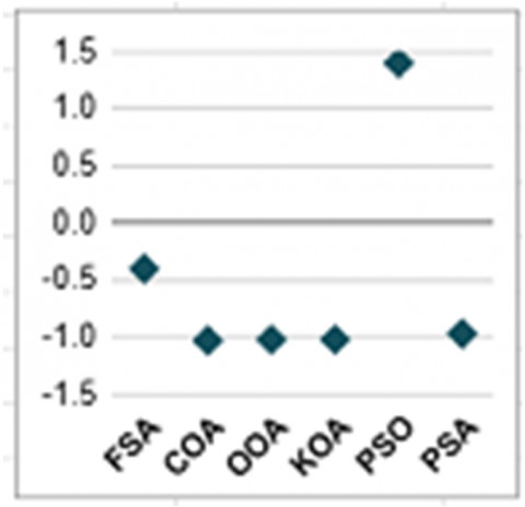
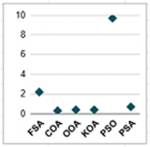
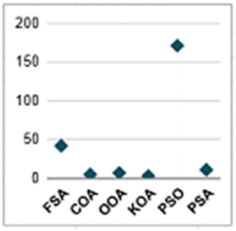
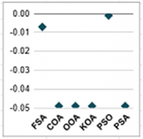
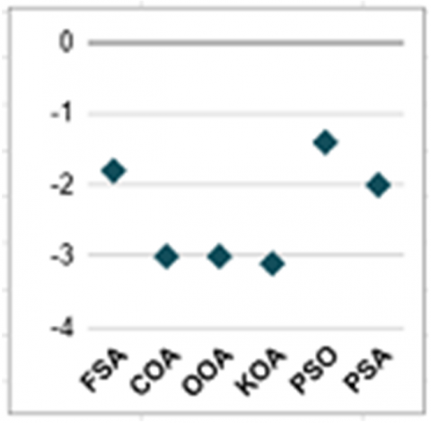
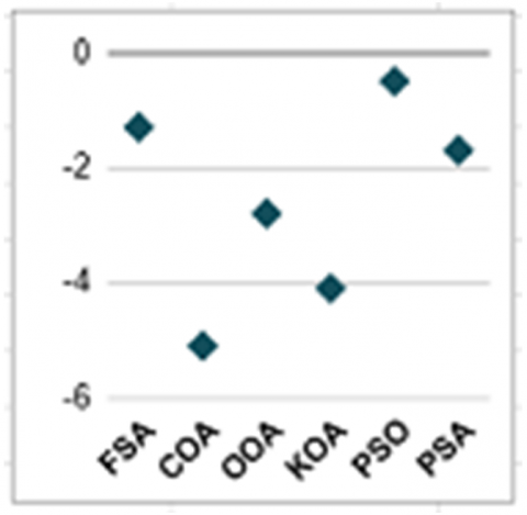
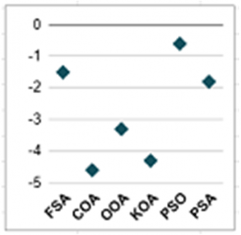
The 23 standard functions are picked due to their coverage. A total of 23 benchmark functions is categorized into three distinct classes. The first class includes seven unimodal problems in high-dimensional space, mainly used to assess the algorithm’s ability to perform exploitation. The second class is made up of six high-dimensional multimodal problems that serve to evaluate exploration capability. The last class contains ten multimodal problems with fixed dimensionality, aimed at analyzing how well an algorithm maintains a balance between exploration and exploitation. For the high-dimensional cases, the dimensionality is set at 50. The outcomes are summarized in Tables 1-4, while Figure 2 illustrates their visual representation. The detailed description of these functions can be found in a previous study [33], including the function declaration, dimension, and boundaries.
|
F1 |
F2 |
F3 |
F4 |
|
F5 |
F6 |
F7 |
F8 |
|
F9 |
F10 |
F11 |
F12 |
|
F13 |
F14 |
F15 |
F16 |
|
F17 |
F18 |
F19 |
F20 |
|
|
|||
|
F21 |
F22 |
F23 |
|
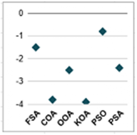
Figure 2. Visualization of the average score on solving 23 functions
Table 1. Result of solving seven HDUFs
|
F |
Parameter |
FSA [23] |
COA [15] |
OOA [17] |
KOA [16] |
PSO [44] |
PSA |
|
1 |
Mean |
4.936 × 10⁴ |
2.094 |
0.748 |
0.574 |
4.524 × 10⁴ |
0.000 |
|
Std. deviation |
8.856 × 10³ |
1.432 |
0.776 |
0.308 |
7.255 × 10³ |
0.000 |
|
|
Mean rank |
6 |
4 |
3 |
2 |
5 |
1 |
|
|
2 |
Mean |
0.000 |
0.000 |
0.000 |
0.000 |
5.115 × 1060 |
0.000 |
|
Std. deviation |
0.000 |
0.000 |
0.000 |
0.000 |
1.935 × 1061 |
0.000 |
|
|
Mean rank |
1 |
1 |
1 |
1 |
6 |
1 |
|
|
3 |
Mean |
1.490 × 10⁵ |
6.839 × 10³ |
4.539 × 10³ |
9.573 × 10³ |
4.093 × 10⁵ |
0.000 |
|
Std. deviation |
6.283 × 10⁴ |
8.098 × 10³ |
3.398 × 10³ |
7.119 × 10³ |
3.362 × 10⁵ |
0.000 |
|
|
Mean rank |
5 |
3 |
2 |
4 |
6 |
1 |
|
|
4 |
Mean |
7.050 × 101 |
3.963 |
1.574 |
5.607 |
6.561 × 101 |
0.000 |
|
Std. deviation |
7.229 |
1.001 |
0.590 |
1.524 × 101 |
5.243 |
0.000 |
|
|
Mean rank |
6 |
3 |
2 |
4 |
5 |
1 |
|
|
5 |
Mean |
1.065 × 10⁸ |
1.192 × 10² |
5.723 × 101 |
5.693 × 101 |
8.654 × 10⁷ |
4.896 × 101 |
|
Std. deviation |
9.648 × 10⁷ |
4.531 × 101 |
5.947 |
5.332 |
2.190 × 10⁷ |
0.016 |
|
|
Mean rank |
6 |
4 |
3 |
2 |
5 |
1 |
|
|
6 |
Mean |
4.432 × 10⁴ |
1.485 × 101 |
1.158 × 101 |
1.144 × 101 |
4.247 × 10⁴ |
1.119 × 101 |
|
Std. deviation |
9.648 × 10³ |
1.596 |
0.810 |
0.594 |
5.860 × 10³ |
0.405 |
|
|
Mean rank |
6 |
4 |
3 |
2 |
5 |
1 |
|
|
7 |
Mean |
8.482 × 101 |
0.068 |
0.049 |
0.037 |
6.687 × 101 |
0.008 |
|
Std. deviation |
3.072 × 101 |
0.033 |
0.021 |
0.019 |
2.624 × 101 |
0.005 |
|
|
Mean rank |
6 |
4 |
3 |
2 |
5 |
1 |
Table 2. Result of solving six HDMFs
|
F |
Parameter |
FSA [23] |
COA [15] |
OOA [17] |
KOA [16] |
PSO [44] |
PSA |
|
8 |
Mean |
-3.539 × 10³ |
-4.441 × 10³ |
-4.148 × 10³ |
-3.935 × 10³ |
-2.665 × 10³ |
-3.140 × 10³ |
|
Std. deviation |
7.082 × 10² |
7.146 × 10² |
5.766 × 10² |
5.725 × 10² |
7.138 × 10² |
3.952 × 10² |
|
|
Mean rank |
4 |
1 |
2 |
3 |
6 |
5 |
|
|
9 |
Std. deviation |
5.658 × 10² |
5.350 |
1.174 |
7.069 |
5.745 × 10² |
0.000 |
|
Range |
3.455 × 101 |
6.095 |
2.155 |
8.218 |
3.158 × 101 |
0.000 |
|
|
Mean rank |
5 |
3 |
2 |
4 |
6 |
1 |
|
|
10 |
Mean |
1.944 × 101 |
0.575 |
0.192 |
0.815 |
1.858 × 101 |
0.000 |
|
Std. deviation |
0.810 |
0.208 |
0.082 |
2.339 |
0.364 |
0.000 |
|
|
Mean rank |
6 |
3 |
2 |
4 |
5 |
1 |
|
|
11 |
Mean |
4.416 × 10² |
0.528 |
0.133 |
0.187 |
4.198 × 10² |
0.000 |
|
Std. deviation |
9.894 × 101 |
0.309 |
0.171 |
0.165 |
6.925 × 101 |
0.000 |
|
|
Mean rank |
6 |
4 |
2 |
3 |
5 |
1 |
|
|
12 |
Mean |
1.343 × 10⁸ |
1.205 |
1.067 |
1.143 |
1.022 × 10⁸ |
1.137 |
|
Std. deviation |
6.048 × 10⁷ |
0.185 |
0.154 |
0.111 |
5.567 × 10⁷ |
0.110 |
|
|
Mean rank |
6 |
4 |
1 |
3 |
5 |
2 |
|
|
13 |
Mean |
2.923 × 10⁸ |
4.155 |
3.532 |
3.544 |
2.547 × 10⁸ |
3.136 |
|
Std. deviation |
1.578 × 10⁸ |
0.593 |
0.165 |
0.160 |
8.511 × 10⁷ |
0.001 |
|
|
Mean rank |
6 |
4 |
2 |
3 |
5 |
1 |
Table 3. Result of solving ten FDMFs
|
F |
Parameter |
FSA [23] |
COA [15] |
OOA [17] |
KOA [16] |
PSO [44] |
PSA |
|
14 |
Mean |
2.129 × 101 |
4.936 |
8.277 |
9.162 |
5.185 × 101 |
9.398 |
|
Std. deviation |
2.731 × 101 |
3.644 |
3.231 |
5.191 |
1.055 × 10² |
3.421 |
|
|
Mean rank |
5 |
1 |
2 |
3 |
6 |
4 |
|
|
15 |
Std. deviation |
0.035 |
0.007 |
0.004 |
0.005 |
0.767 |
0.004 |
|
Range |
0.026 |
0.011 |
0.004 |
0.007 |
0.834 |
0.005 |
|
|
Mean rank |
5 |
4 |
1 |
3 |
6 |
1 |
|
|
16 |
Mean |
-0.443 |
-1.030 |
-1.026 |
-1.021 |
1.429 |
-0.978 |
|
Std. deviation |
0.858 |
0.001 |
0.010 |
0.013 |
6.011 |
0.098 |
|
|
Mean rank |
5 |
1 |
2 |
3 |
6 |
4 |
|
|
17 |
Mean |
2.277 |
0.399 |
0.402 |
0.402 |
9.730 |
0.736 |
|
Std. deviation |
3.422 |
0.002 |
0.010 |
0.004 |
1.129 × 101 |
0.346 |
|
|
Mean rank |
5 |
1 |
2 |
2 |
6 |
4 |
|
|
18 |
Mean |
4.277 × 101 |
5.172 |
7.138 |
3.103 |
1.717 × 10² |
1.130 × 101 |
|
Std. deviation |
3.513 × 101 |
6.273 |
9.761 |
0.249 |
2.135 × 10² |
1.556 × 101 |
|
|
Mean rank |
5 |
2 |
3 |
1 |
6 |
4 |
|
|
19 |
Mean |
-0.007 |
-0.049 |
-0.049 |
-0.049 |
-0.001 |
-0.049 |
|
Std. deviation |
0.013 |
0.000 |
0.000 |
0.000 |
0.003 |
0.000 |
|
|
Mean rank |
5 |
1 |
1 |
1 |
6 |
1 |
|
|
20 |
Std. deviation |
-1.816 |
-3.093 |
-3.068 |
-3.142 |
-1.411 |
-2.083 |
|
Range |
0.778 |
0.124 |
0.144 |
0.074 |
0.712 |
0.415 |
|
|
Mean rank |
5 |
2 |
3 |
1 |
6 |
4 |
|
|
21 |
Mean |
-1.308 |
-5.189 |
-2.829 |
-4.166 |
-0.585 |
-1.781 |
|
Std. deviation |
1.242 |
2.379 |
1.320 |
1.321 |
0.263 |
0.951 |
|
|
Mean rank |
5 |
1 |
3 |
2 |
6 |
4 |
|
|
22 |
Mean |
-1.552 |
-4.623 |
-3.353 |
-4.352 |
-0.643 |
-1.848 |
|
Std. deviation |
0.812 |
2.283 |
1.735 |
1.265 |
0.209 |
0.979 |
|
|
Mean rank |
5 |
1 |
3 |
2 |
6 |
4 |
|
|
23 |
Mean |
-1.528 |
-3.852 |
-2.540 |
-3.971 |
-0.866 |
-2.468 |
|
Std. deviation |
0.957 |
1.687 |
1.032 |
1.578 |
0.271 |
1.191 |
|
|
MEAN rank |
5 |
2 |
3 |
1 |
6 |
4 |
Table 4. Summary results of the supremacy of PSA in solving 23 functions
|
Group |
FSA [23] |
COA [15] |
OOA [17] |
KOA [16] |
PSO [44] |
|
1 |
6 |
6 |
6 |
6 |
7 |
|
2 |
5 |
5 |
4 |
5 |
6 |
|
3 |
10 |
1 |
0 |
1 |
10 |
|
Total |
21 |
12 |
10 |
12 |
23 |
Although PSA remains competitive for fixed-dimension multimodal functions, it does not outperform other methods, as illustrated in Table 3. PSA ranks fourth in ten functions (F14, F16–F18, F20–F23) and holds the top position in two functions (F15 and F19). In the case of F15, OOA matches PSA’s performance. For F19, PSA shares the highest score with three additional algorithms: COA, OOA, and KOA. Across all ten functions, PSO consistently yields the poorest outcomes, while FSA ranks just above it with the second-lowest performance. The difference among algorithms in each function is also narrow, except in F15.
Table 4 highlights PSA’s strong performance across 23 benchmark functions. Compared to other methods, PSA outperforms FSA in 21 functions, COA in 12, OOA in 10, KOA in 12, and PSO in all 23 cases. Root in this result, PSA is better than FSA and PSO in three groups of functions. Meanwhile, PSA is better than COA, OOA, and KOA only in the high-dimensional functions.
There are two cases of ELD problem that are used in this research. In the initial scenario, a system composed of six units is analysed, whereas the subsequent scenario involves a system with ten units. The detailed description of the six-unit system can be found in reference [12], while the ten-unit system can be found in reference [41]. This description includes the cost constant and power range for the generating units. The outcomes are summarized in Tables 5-8. Specifically, Tables 5 and 6 present the findings for the six-unit configuration, while Tables 7 and 8 display the results for the ten-unit system. Table 5 and Table 7 provide five parameters for the result for the total cost, including average standard deviation, minimum, maximum, and mean rank. On the other hand, Table 6 and Table 8 provide the detailed results for the best scenario for every algorithm: the power that is produced by every generator and the total cost root in this scenario.
The findings indicate that PSA performs effectively in addressing both scenarios of the ELD challenge. PSA is placed in the third rank in the 6-unit system and in the fourth rank in the 10-unit system. KOA becomes the best algorithm in the 6-unit system while OOA becomes the best algorithm in the 10-unit system. FSA becomes the second-worst algorithm in both systems, while PSO becomes the worst algorithm in both systems. The result also shows the very competitive circumstances in handling both cases, as the difference among algorithms is very narrow.
Table 5. Result of solving 6-unit system
|
Algorithm |
Average ($) |
Std-dev ($) |
Min ($) |
Max ($) |
Rank |
|
FSA [23] |
12,230 |
77 |
12,157 |
12,487 |
5 |
|
COA [15] |
12,157 |
3 |
12,152 |
12,164 |
2 |
|
OOA [17] |
12,185 |
17 |
12,161 |
12,234 |
4 |
|
KOA [16] |
12,156 |
3 |
12,151 |
12,167 |
1 |
|
PSO [44] |
12,262 |
47 |
12,215 |
12,399 |
6 |
|
PSA |
12,172 |
12 |
12,155 |
12,201 |
3 |
Table 6. Best result of solving 6-unit system
|
Parameter |
FSA [23] |
COA [15] |
OOA [17] |
KOA [16] |
PSO [44] |
PSA |
|
G1 (MW) |
500 |
500 |
500 |
500 |
492 |
500 |
|
G2 (MW) |
183 |
151 |
179 |
156 |
151 |
166 |
|
G3 (MW) |
260 |
261 |
270 |
251 |
222 |
240 |
|
G4 (MW) |
107 |
119 |
120 |
116 |
112 |
104 |
|
G5 (MW) |
158 |
156 |
144 |
166 |
185 |
168 |
|
G6 (MW) |
55 |
76 |
50 |
74 |
101 |
85 |
|
Cost ($) |
12,157 |
12,152 |
12,161 |
12,151 |
12,215 |
12,155 |
Table 7. Result of solving 10-unit system
|
Algorithm |
Average ($) |
Std-dev ($) |
Min ($) |
Max ($) |
Rank |
|
FSA [23] |
97,284 |
2,262 |
95,669 |
105,847 |
5 |
|
COA [15] |
96,132 |
345 |
95,686 |
97,181 |
3 |
|
OOA [17] |
95,894 |
182 |
95,685 |
96,381 |
1 |
|
KOA [16] |
96,050 |
303 |
95,673 |
96,881 |
2 |
|
PSO [44] |
99,898 |
3,107 |
96,892 |
106,577 |
6 |
|
PSA |
96,739 |
737 |
95,842 |
98,694 |
4 |
Table 8. Best result of solving 10-unit system
|
Parameter |
FSA [23] |
COA [15] |
OOA [17] |
KOA [16] |
PSO [44] |
PSA |
|
G1 (MW) |
37 |
40 |
33 |
31 |
83 |
23 |
|
G2 (MW) |
50 |
46 |
45 |
51 |
58 |
45 |
|
G3 (MW) |
188 |
178 |
186 |
189 |
165 |
168 |
|
G4 (MW) |
132 |
143 |
136 |
131 |
109 |
141 |
|
G5 (MW) |
10 |
10 |
14 |
12 |
20 |
10 |
|
G6 (MW) |
10 |
10 |
10 |
10 |
16 |
10 |
|
G7 (MW) |
23 |
23 |
23 |
23 |
23 |
23 |
|
G8 (MW) |
26 |
29 |
28 |
30 |
46 |
33 |
|
G9 (MW) |
23 |
23 |
23 |
23 |
23 |
23 |
|
G10 (MW) |
117 |
114 |
118 |
116 |
73 |
140 |
|
Cost ($) |
95,669 |
95,686 |
95,685 |
95,673 |
96,892 |
95,842 |
In general, the findings indicate that PSA can be considered a viable approach for optimization tasks. The result shows that the exploration and exploitation capabilities of PSA are superior while its balancing competence between both exploitation and exploration is competitive. Meanwhile, PSA is absolute superior compared to FSA and PSO.
The performance gap among algorithms when applied to 23 benchmark functions is closely linked to the variation observed between their top and bottom outcomes. Specifically, for high-dimensional unimodal functions, six of them (F1–F6) exhibit a substantial disparity between the highest and lowest results, whereas F7 shows only a slight difference. The difference between the best and worst results is wide in three functions (F8, F11, and F12), moderate in two functions (F9 and F10), and narrow in F13. In the case of fixed-dimension multimodal functions, four functions (F14, F15, F17, and F18) exhibit a large gap between their highest and lowest outcomes, whereas six functions (F16, F19–F23) show only a small variation. This observation highlights the tendency for high-dimensional functions to produce widely varying results, while functions with a fixed dimension generally yield more consistent outcomes.
The superiority of PSA in handling high dimension functions can also be traced root in the nature of the terrain in high dimension functions. In general, the terrain of these high dimension functions is clear except in F8. Moreover, the global optimal also lies in the area in the center of the solution space, except in F8. In F8, the general terrain is very wavy and the trend for the location of the global optimal is ambiguous so that it is difficult to trace. Conversely, in multimodal problems with a fixed number of variables, the landscape tends to be less clear, typically resembling a level surface where the region containing the global optimum is extremely limited. It makes it difficult for the algorithm with stringent acceptance approach to improve its solution as the probability for improvement is low so that the probability of an agent staying in its current location is high due to high probability of stagnation.
Very competitive situation in the ELD problems can be related to the constraints. As provided in reference [12], the demand for the 6-unit system is 1,263 MW. Meanwhile the minimum total power is 300 MW while the maximum total power is 1,470 MW. It means that the demand is 86 percent of the maximum total power while the minimum total power is 26 percent of the maximum total power. It means that although the power range is wide enough, the actual solution space is narrow as almost all generators must be set near their maximum power. Moreover, the maximum power of generator G1 is 500 MW which is almost one-third of the maximum total power so that it is impossible for the power of G1 to be set low. The same circumstance also occurs in the 10-unit system. The demand is 616 MW. On the other hand, the minimum total power is 271.25 MW while the maximum total power is 1,094 MW. It means that the demand is 56 percent of the maximum total power while the minimum total power is 25 percent of the maximum total power. It makes the actual solution space of the 10-unit system narrow too although it is not so narrow as the 6-unit system. Wider actual solution space in 10-unit system rather than the 6-unit system makes the standard deviation of the result in 10-unit system is much higher than the 6-unit system. This fact shows that in the ELD problem, the actual solution space becomes more dominant than the algorithm which makes even the superior algorithm lose its superiority in handling ELD problems.
This research has provided a new metaheuristic-algorithm called PSA. It has specific nature including free from metaphor and multiple-search approach. Detailed description and investigation of its effectiveness also have been provided. The findings indicate that PSA outperforms FSA, COA, OOA, KOA, and PSO in 21, 12, 10, 12, and 23 of the 23 tested functions, respectively. It is concluded that FSA is superior to FSA and PSO in most of the 23 functions. PSA is competitive in solving both cases of ELD problems as it becomes the third best in the 6-unit system and fourth best in the 10-unit system. The result also shows that ELD problem is highly competitive as there is not any technique that performs superiorly compared to other techniques with significant gap.
In the future, PSA can be implemented to solve numerous other ED problems or in the broader context, wider practical optimization problems in engineering fields, such as manufacturing system, supply chain system, transportation, and so on.
|
a |
action |
|
blow |
lower boundary |
|
bup |
upper boundary |
|
c |
solution candidate |
|
d |
dimension |
|
e |
cost |
|
etot |
total cost |
|
f |
objective function |
|
g |
generator or power of generator |
|
G |
set of generators |
|
gmin |
minimum power |
|
gmax |
maximum power |
|
oELD |
objective function for ELD problem |
|
P |
set of bigger agents |
|
r1 |
uniform random [0,1] |
|
r2 |
uniform random from a set |
|
r3 |
uniform random [0, 0.5] |
|
s |
constants for ELD cost function |
|
x |
agent |
|
X |
set of agents |
|
xbgt |
the biggest agent |
|
xsel |
selected agent |
|
t |
iteration |
|
T |
maximum iteration |
|
W |
set of smaller agents |
|
Subscripts |
|
|
i |
index for agent |
|
j |
index for dimension or dimension or generator |
|
n |
cardinality |
|
m |
dimension size |
[1] Muppidi, R., Nuvvula, R.S.S., Muyeen, S.M., Shezan, S.K.A., Ishraque, M.F. (2022). Optimization of a fuel cost and enrichment of line loadability for a transmission system by using rapid voltage stability index and grey wolf algorithm technique. Sustainability, 14(7): 4347. https://doi.org/10.3390/su14074347
[2] Ding, F., Liu, M., Hsiang, S.M., Hu, P., Zhang, Y.X., Jiang, K.W. (2024). Duration and labor resource optimization for construction projects—A conditional-value-at-risk-based analysis. Buildings, 14(2): 553. https://doi.org/10.3390/buildings14020553
[3] Abadi, M.F., Bordbari, M.J., Haghighat, F., Nasiri, F. (2025). Dynamic maintenance cost optimization in data centers: An availability-based approach for K-out-of-N systems. Buildings, 15(7): 1057. https://doi.org/10.3390/buildings15071057
[4] Song, H., Chen, X.X., Wang, H.P. (2024). Carbon emission optimization for assembled buildings using interval grey GERT modelling and modify NSGA-III algorithm in China. KCSE Journal of Civil Engineering, 28: 5415-5426. https://doi.org/10.1007/s12205-024-2619-6
[5] Koch, L., da Silva, F.J.G., Campilho, R.D.S., de Sa, J.C.V., Lucas, R.R., Sales-Contini, R.C.M. (2025). Mitigation strategies for waste elimination and cost reduction in the manufacture of Bowden cables. The International Journal of Advanced Manufacturing Technology, 137: 4143-4167. https://doi.org/10.1007/s00170-025-15367-4
[6] Jia, Z.H., Jia, Y.F., Liu, C., Xu, G.M., Li, K. (2024). A self-learning multi-population evolutionary algorithm for flexible job shop scheduling under time-of-use pricing. Computers & Industrial Engineering, 189: 110004. https://doi.org/10.1016/j.cie.2024.110004
[7] Liu, S.Q., Zhu, H.P., Sheng, L.Z. (2026). Integrated dynamic scheduling method for hybrid flow shop with machine preventive maintenance based on cooperative multi-agent deep reinforcement learning. Robotics and Computer-Integrated Manufacturing, 97: 103085. https://doi.org/10.1016/j.rcim.2025.103085
[8] Soto-Concha, R., Escobar, J.W., Morillo-Torres, D., Linfati, R. (2025). The vehicle-routing problem with satellites utilization: A systematic review of the literature. Mathematics, 13(7): 1092. https://doi.org/10.3390/math13071092
[9] Khodashenas, S., Abtahi, Z., Saahraeian, R. (2026). The cost and time objectives minimization in cross-dock truck scheduling of perishable goods considering uncertainty. International Journal of Engineering, 39(2): 492-510. https://doi.org/10.5829/ije.2026.39.02b.16
[10] Das, T., Roy, R., Mandal, K.K. (2025). Solving the cost minimization problem of optimal reactive power dispatch in a renewable energy integrated distribution system using rock hyraxes swarm optimization. Electrical Engineering, 107: 741-773. https://doi.org/10.1007/s00202-024-02548-9
[11] Bulbul, S.M.A., Pradhan, M., Roy, P.K., Pal, T. (2018). Opposition-based krill herd algorithm applied to economic load dispatch problem. Ain Shams Engineering Journal, 9: 423-440. https://doi.org/10.1016/j.asej.2016.02.003
[12] Hassan, M.H., Kamel, S., Eid, A., Nasrat, L., Jurado, F., Elnaggar, M.F. (2023). A developed eagle-strategy supply-demand optimizer for solving economic load dispatch problems. Ain Shams Engineering Journal, 14: 102083. https://doi.org/10.1016/j.asej.2022.102083
[13] Puspitasari, K.M.D., Raharjo, J., Sastrosubroto, A.S., Rahmat, B. (2022). Generator scheduling optimization involving emission to determine emission reduction costs. International Journal of Engineering, 35(8): 1468-1478. https://doi.org/10.5829/ije.2022.35.08b.02
[14] Zein, H., Raharjo, J., Mardiyanto, I.R. (2022). A method for completing economic load dispatch using the technique of narrowing down area. IEEE Access, 10: 30822-30831. https://doi.org/10.1109/ACCESS.2022.3158928
[15] Dehghani, M., Montazeri, Z., Trojovská, E., Trojovský, P. (2023). Coati optimization algorithm: A new bio-inspired metaheuristic algorithm for solving optimization problems. Knowledge-Based Systems, 259: 110011. https://doi.org/10.1016/j.knosys.2022.110011
[16] Dehghani, M., Montazeri, Z., Bektemyssova, G., Malik, O.P., Dhiman, G., Ahmed, A.E.M. (2023). Kookaburra optimization algorithm: A new bio-inspired metaheuristic algorithm for solving optimization problems. Biomimetics, 8(6): 470. https://doi.org/10.3390/biomimetics8060470
[17] Dehghani, M., Trojovský, P. (2023). Osprey optimization algorithm: A new bio-inspired metaheuristic algorithm for solving engineering optimization problems. Frontiers in Mechanical Engineering, 8: 1126450. https://doi.org/10.3389/fmech.2022.1126450
[18] Suyanto, S., Ariyanto, A.A., Ariyanto, A.F. (2022). Komodo mlipir algorithm. Applied Soft Computing, 114: 108043. https://doi.org/10.1016/j.asoc.2021.108043
[19] Chopra, N., Ansari, M.M. (2022). Golden jackal optimization: A novel nature-inspired optimizer for engineering applications. Expert Systems With Applications, 198: 116294. https://doi.org/10.1016/j.eswa.2022.116924
[20] Trojovska, E., Dehghani, M., Trojovsky, P. (2022). Fennec fox optimization: A new nature-inspired optimization algorithm. IEEE Access, 10: 84417-84443. https://doi.org/10.1109/ACCESS.2022.3197745
[21] Hamadneh, T., Batiha, B., Werner, F., Montazeri, Z., Dehghani, M., Bektemyssova, G., Eguchi, K. (2024). Fossa optimization algorithm: A new bio-inspired metaheuristic algorithm for engineering applications. International Journal of Intelligent Engineering and Systems, 17(5): 1038-1047. https://doi.org/10.22266/ijies2024.1031.78
[22] Hamadneh, T., Batiha, B., Al-Refai, O., Ibraheem, I.K., Smerat, A., Werner, F., Montazeri, Z., Dehghani, M., Jawad, R.K., Al-Salih, A.A.M.M, Ahmed, M.A., Eguchi, K. (2025). Salamander optimization algorithm: A new bio-inspired approach for solving optimization problems. International Journal of Intelligent Engineering and Systems, 18(7): 550-562. https://doi.org/10.22266/ijies2025.0831.35
[23] Hamadneh, T., Batiha, B., Al-Refai, O., Ibraheem, I.K., Smerat, A., Montazeri, Z., Dehghani, M., Jawad, R.K., Zalzala, A.M., Al-Salih, A.A.M.M., Ahmed, M.A., Eguchi, K. (2025). Farmer and seasons algorithm (FSA): A parameter-free seasonal metaheuristic for global optimization. International Journal of Intelligent Engineering and Systems, 18(6): 947-960. https://doi.org/10.22266/ijies2025.0731.59
[24] Hamadneh, T., Batiha, B., Al-Refai, O., Montazeri, Z., Dehghani, M., Aribowo, W., Ibrahim, M.K., Jawad, R.K., Al-Salih, A.A.M.M., Ahmed, M.A., Ibraheem, I.K., Eguchi, K. (2025). Motorbike courier optimization: a novel parameter-free metaheuristic for solving constrained real-world optimization problems. International Journal of Intelligent Engineering and Systems, 18(5): 382-393. https://doi.org/10.22266/ijies2025.0630.27
[25] Kusuma, P.D., Adiputra, D. (2022). Modified social forces algorithm: From pedestrian dynamic to metaheuristic optimization. International Journal of Intelligent Engineering and Systems, 15(3): 294-303. https://doi.org/10.22266/ijies2022.0630.25
[26] Dehghani, M., Mardaneh, M., Guerrero, J.M., Malik, O.P., Ramirez-Mendoza, R.A., Matas, J., Vasquez, J.C., Parra-Arroyo, L. (2020). A new “doctor and patient” optimization algorithm: An application to energy commitment problem. Applied Sciences, 10(17): 5791. https://doi.org/10.3390/app10175791
[27] Oladejo, S.O., Ekwe, S.O., Akinyemi, L.A., Mirjalili, S.A. (2023). The deep sleep optimizer: A human-based metaheuristic approach. IEEE Access, 11: 83639-83665. https://doi.org/10.1109/ACCESS.2023.3298105
[28] Hamadneh, T., Batiha, B., Al-Refai, O., Ibraheem, I.K., et al. (2025). Program manager optimization algorithm: A new method for engineering applications. International Journal of Intelligent Engineering and Systems, 18(7): 746-756. https://doi.org/10.22266/ijies2025.0831.47
[29] Ghasemi, M., Rahimnejad, A., Akbari, E., Rao, R.V., Trojovský, P., Trojovská, E., Gadsden, S.A. (2023). A new metaphor-less simple algorithm based on Rao algorithms: A fully informed search algorithm (FISA). PeerJ Computer Science, 9: e1431. https://doi.org/10.7717/peerj-cs.1431
[30] Trojovský, P., Dehghani, M. (2023). Subtraction-average-based optimizer: A new swarm-inspired metaheuristic algorithm for solving optimization problems. Biomimetics, 8(2): 149. https://doi.org/10.3390/biomimetics8020149
[31] Dehghani, M., Hubálovský, Š., Trojovský, P. (2022). A new optimization algorithm based on average and subtraction of the best and worst members of the population for solving various optimization problems. PeerJ Computer Science, 8: e910. https://doi.org/10.7717/peerj-cs.910
[32] Kusuma, P.D. (2025). Adaptive group algorithm: An adaptive metaheuristic based on the improvement of the group. Intelligent Engineering and Systems, 18(3): 91-104. https://doi.org/10.22266/ijies2025.0430.07
[33] Noroozi, M., Mohammadi, H., Efatinasab, E., Lashgari, A., Eslami, M., Khan, B. (2022). Golden search optimization algorithm. IEEE Access, 10: 37515-37532. https://doi.org/10.1109/ACCESS.2022.3162853
[34] Al-Betar, M.A., Awadallah, M.A., Zitar, R.A., Assaleh, K. (2023). Economic load dispatch using memetic sine cosine algorithm. Journal of Ambient Intelligence and Humanized Computing, 14: 11685-11713. https://doi.org/10.1007/s12652-022-03731-1
[35] Al-Kubragyi, S.S.A., Ali, I.I. (2025). A hybrid moth flam algorithm based on particle swarm optimization for unit commitment problem solving. Journal Européen des Systèmes Automatisés, 58(1): 39-45. https://doi.org/10.18280/jesa.580105
[36] Xiong, G.J., Liu, Q.H., Wang, Y., Fu, X.F. (2025). Power system economic emission dispatch considering uncertainties of wind, solar, and small runoff hydropower via a hybrid multi-objective optimization algorithm. Expert Systems with Applications, 278: 127375. https://doi.org/10.1016/j.eswa.2025.127375
[37] Sepuldiva, S., Garces-Ruiz, A., Mora-Florez, J. (2024). Generic optimal power flow for active distribution networks. Electrical Engineering, 106: 3529-3542. https://doi.org/10.1007/s00202-023-02147-0
[38] Spea, S.R. (2025). Cost-effective economic dispatch in large-scale power systems using enhanced manta ray foraging optimization. Neural Computing and Applications, 37: 12487-12524. https://doi.org/10.1007/s00521-025-11086-9
[39] Nagarajan, K., Rajagopalan, A., Bajaj, M., Sitharthan, R., Mohammadi, S.A.D., Blazek, V. (2024). Optimizing dynamic economic dispatch through an enhanced cheetah‑inspired algorithm for integrated renewable energy and demand‑side management. Scientitifc Reports, 14: 3091. https://doi.org/10.1038/s41598-024-53688-8
[40] Hassan, M.H., Kamel, S., Selim, A., Shaheen, A., Yu, J., El-Sehiemy, R. (2024). Efficient economic operation based on load dispatch of power systems using a leader white shark optimization algorithm. Neural Computing and Applications, 36: 10613-10635. https://doi.org/10.1007/s00521-024-09612-2
[41] Tariq, F., Alelyani, S., Abbas, G., Qahmash, A., Hussain, M.R. (2020). Solving renewables-integrated economic load dispatch problem by variant of metaheuristic bat-inspired algorithm. Energies, 13: 6225. https://doi.org/10.3390/en13236225
[42] Secui, D.C., Bendea, G., Secui, M.L., Hora, C., Bendea, C. (2021). The chaotic social group optimization for the economic dispatch problem. International Journal of Inteligent Engineering and Systems, 14(6): 666-677. https://doi.org/10.22266/ijies2021.1231.59
[43] Singh, N., Chakrabarti, T., Chakrabarti, P., Margala, M., Gupta, A., Praveen, S.P., Khrisnan, S.B., Unhelkar, B. (2023). Novel heuristic optimization technique to solve economic load dispatch and economic emission load dispatch problems. Electronics, 12: 2921. https://doi.org/10.3390/electronics12132921
[44] Gad, A.G. (2022). Particle swarm optimization algorithm and its applications: A systematic review. Archives of Computational Methods in Engineering, 29: 2531-2561. https://doi.org/10.1007/s11831-021-09694-4