Stefano Morchio*![]() | Marco Fossa
| Marco Fossa![]() | Samuele Memme
| Samuele Memme![]() | Antonella Priarone
| Antonella Priarone![]()
© 2025 The authors. This article is published by IIETA and is licensed under the CC BY 4.0 license (http://creativecommons.org/licenses/by/4.0/).
OPEN ACCESS
The methods used for designing vertical borehole heat exchanger (BHE) fields in ground-coupled heat pump (GCHP) applications require sets of input parameters to know and assign. While the reference methods commonly consider the 10-year horizon in the design of the BHE fields as a standard, the proposed (Tp8) method has been extended to cover both the 10-year and 25-year horizon designs. This method has been extensively validated through comparisons with commercial software in a wide range of design test cases. The method is made available and packaged as a comprehensive and free web-based design tool, offering BHE field design for both 10-year and 25-year horizons. This paper presents the features of the online design tool and highlights the main factors distinguishing the two different time horizon designs. Analyses on how different building heat load profiles primarily affect the BHE field designs have been reported. Given the building heat load profile and related peak loads reported at the ground side, the correct overall borehole length evaluated at each design time horizon relies on the correct estimates of ground thermal conductivity and borehole thermal resistance. The average increase in the overall borehole length between the 10th and 25th year is 14%.
borehole heat exchangers, design, energy efficiency, ground-coupled heat pumps
The proper design of borehole heat exchanger (BHE) fields used in ground-coupled heat pump (GCHP) applications assumes a key role in preserving the correct operability of the system. Each design method of BHE fields in GCHP applications requires a series of inputs. Among these inputs, there are the undisturbed ground temperature, the borehole and ground thermal properties, the choice of the BHE field configuration, i.e., the number and spacing of BHEs, and the pipe geometry. One of the most important inputs, sensibly affecting the design of BHE fields, is the building heat demand expressed in terms of a monthly heat load profile over a year and related peak loads in heating and cooling. By setting the desired Coefficient of Performance (COP) according to the geothermal carrier fluid temperature limits that cannot be overridden at the end of the considered time horizon, it is possible to correctly design the BHE field.
The ASHRAE method (also adopted by the Italian Technical Standard, UNI 11466), originally introduced by Kavanaugh and Rafferty [1], is one of the simplest algorithms for BHE field design. This method depends on the above-mentioned inputs and requires a reliable model for calculating the Temperature Penalty (Tp), which accounts for the thermal response of the borefield configuration using the g-function approach. In this method, the annual building heat load profile is condensed into three simplified heat pulses applied to the ground: 10 years of the yearly averaged heat load, 1 month of the most demanding monthly heat load, and 6 hours for the peak heat load of the most demanding month.
The method evaluates the ground’s thermal response as the time superposition of the solutions corresponding to the three aggregated heat pulses employing the Infinite Cylindrical Source (ICS) model [2]. However, since the ICS model does not account for 2D and 3D heat transfer effects in the ground, the corrective parameter Tp is introduced to improve long-term accuracy.
Several refinements to the original ASHRAE method have been developed. Fossa et al. [3] maintained the original ASHRAE formulation in their ASHRAE-Tp8 method but significantly enhanced the Tp calculation. Their approach introduced optimized constants tailored to different BHE field arrangements, derived from a broad analysis of g-functions by Eskilson [4] representing realistic ground thermal responses. The optimized constants are used in the expression for the Tp evaluation in the ASHRAE-Tp8 method.
All methods that deviate from the standard ASHRAE approach, such as those proposed by Ahmadfard and Bernier [5] and Fossa et al. [3], refine the evaluation of the overall borehole field length by typically assuming a plant lifespan of 10 years. Kurevija et al. [6] and other authors highlight the rising need for design methods and tools to correctly design and guarantee longer-term performance for at least 25 to 30 years. The 25-year horizon has been used in the comparison between coaxial, single and double U BHE configurations in terms of thermal and hydraulic performance reported in the recent study by Brown et al. [7]. Comparisons between a fully discretized 3D numerical BHE model, a resistance-capacitance (RC) model, a g-function model, and a hybrid model — against real-world monitoring data are provided by Heim et al. [8]. Three novel approaches to size geothermal borefields (energy piles) within a mixed-integer-linear-problem (MILP) framework, including a complex g-function-based model, have been proposed by Blanke et al. [9]. Their method proves to be particularly useful for large-scale energy system optimization, integrating accurate BHE sizing directly into MILP programming models. The work of Magdic et al. [10] considers the BHE and the rest of the system (heat pump, circulation pump, building) allowing to show that reducing borehole depth (while maintaining heat exchange) can yield more cost-effective savings over a 10-year operational period, without mentioning the results of the same analysis in terms of costs and BHE thermal performance for a more extended time horizon. The present authors were the first to extend the time horizon for the yearly averaged heat load from 10 to 25 years, covering a plant operability horizon more suitable and appealing for a commercial or residential unit. Thus, they propose the ASHRAE-Tp 825 method that incorporates updated sets of optimized constants. Both the ASHRAE-Tp 810 and ASHRAE-Tp 825 methods have been extensively validated through a wide range of design test cases and related scenarios, including comparisons with commercial software [11, 12]. The method is now available as a free web-based design tool named BHEDesigner8, accessible at www.geosensingdesign.org, offering comprehensive BHE field design for both 10-year and 25-year planning horizons.
Comprehensive descriptions of the ASHRAE-Tp 810 and ASHRAE-Tp 825 methods, in particular, how the optimized constants have been obtained and how different shapes of the building heat load profile can affect the BHE field design for the 10-year and 25-year horizons, have been widely discussed in already published papers by the authors [11, 12].
This paper presents the key features of the online design tool and highlights the main factors distinguishing 10-year and 25-year designs. In particular, it discusses how the two different time horizon designs can be affected primarily by the yearly and peak heat loads, and variations in the estimated borehole thermal resistance (Rb) and ground thermal conductivity (kgr). As evidenced in some reported cases, relatively small variations in the estimated kgr and Rb can have a consistent impact across both horizons. In particular, the kgr and Rb and their variations strongly impact the BHE field design determining an increase (or decrease) in the overall borehole length evaluated for each horizon design considered and influencing the level increment of L when evaluated in the 25th year instead of in the 10th year; the spread between the evaluated overall borehole lengths in the two design horizons tends to remain largely unchanged, with some exceptions (related to variations in kgr). Recently, Tarrad [13] provided a correlation for the prediction of the borehole thermal resistance for the preliminary design of the U-tube ground heat exchanger. Ground thermal properties, borehole properties, ground pump parameters and economic considerations on the design and application of deep BHE have been discussed by Chen and Tomac [14].
The novelty and significance of this study lie in the implementation of the ASHRAE-Tp 810 and ASHRAE-Tp 825 methods within the first freely accessible web application designed to determine the required geometry of a BHE field serving a GCHP. Both the ASHRAE-Tp 810 and ASHRAE-Tp 825 methods, incorporated into BHEDesigner8, have demonstrated significantly improved precision compared to the original ASHRAE method while retaining its simplicity. In addition, the effectiveness of the Tp8 approach has been demonstrated by comparing its provided designs with those obtainable by established commercial software tools for BHE field design, such as EED and GLHEPRO [15].
In the present paper, the use of BHEDesigner8 is stressed once more in a series of test cases for both the above-mentioned design horizons. All calculations using the BHEDesigner8 have been performed directly through the free web application developed by the authors, and compared to those provided by the EED software. The case studies included in this analysis cover a wide range of BHE overall lengths and related depths and BHE field configurations, encompassing installations found worldwide.
Given the entire annual monthly step load profile, the standard ASHRAE sizing models consider 3 aggregated thermal loads (in heating and cooling) of the building spanning over 10 years. These aggregated methods employ the ICS solution to tackle the Fourier problem in the conductive medium. This solution is corrected by the “temperature penalty” Tp suitably introduced in the ASHRAE Handbook [16] to account for the thermal response of complex geometry BHE fields, where the thermal interactions between adjacent boreholes and the related 2D and 3D effects in the ground temperature field cannot be disregarded. The Infinite Line Source (ILS) [2, 17] and ICS models for borehole heat transfer provide the reference analytical solutions of the heat conduction equation related to an infinite source injecting a constant and uniform heat transfer rate per unit length $\dot{Q}^{\prime}$ into an infinite medium. The solutions provided by the ILS and ICS (properly corrected by the Tp) constitute the basic foundation of these triple-step design methods and are used in the time superposition of the heat loads reported at the ground side.
As well as the original ASHRAE method, Eq. (1) is the founding equation of the ASHRAE-Tp 810 and ASHRAE-Tp 825 methods, allowing the evaluation of the overall borehole field length L (also described in the previous study [18]):
$L=\frac{\left\{\dot{Q}_y R_y+\dot{Q}_m R_m+\dot{Q}_h\left(R_h+R_b\right)\right\}}{T_{g r, \infty}-T_{f, { ave }}\left(\tau_n\right)-T_p}$ (1)
The symbol $\dot{Q}$ in Eq. (1) is each heat transfer rate transduced at the ground side through the related COP (in heating and/or cooling mode).
$\dot{Q}_y$ is the yearly load; in the case of the ASHRAE-Tp 810 and ASHRAE-Tp 825 is applied to 10 and 25 years, respectively. $\dot{Q}_m$ is the most demanding monthly heat load of the year, and $\dot{Q}_h$ is a heat pulse of 6 hours corresponding to the peak heat load related to the most demanding month. The Tf,ave(τn) is related to the COPpeak at peak operating conditions of the GCHP and is the expected minimum (or maximum) average (inlet and outlet) temperature [℃] of the geothermal carrier fluid at time τn. The time period τn is 10 years + 1 month + 6 hours for the ASHRAE-Tp 810, and 25 years + 1 month + 6 hours for the ASHRAE-Tp 825.
The undisturbed ground temperature [℃] Tgr,∞ can be evaluated by means of a Thermal Response Test (TRT) [19] together with kgr and Rb.
Ry Rm Rh are the thermal resistances [mK/W], evaluated according to the ICS model resulting from writing the time superposition of the related G-functions corresponding to the dimensionless Fourier numbers Foτn, Foτm+h and Foτh, (where τm+h = 1 month + 6 hours, τh = 6 hours) reported in Eqs. (2)-(4) respectively.
$R_y=\frac{G\left(F o_{\tau_n}\right)-G\left(F o_{\tau_{m+h}}\right)}{k_{g r}}$ (2)
$R_m=\frac{G\left(F o_{\tau_{m+h}}\right)-G\left(F o_{\tau_h}\right)}{k_{g r}}$ (3)
$R_h=\frac{G\left(F o_{\tau_h}\right)}{k_{q r}}$ (4)
Finally, Tp is the temperature penalty [℃]. Different models have been proposed to correctly estimate this parameter; the ASHRAE-Tp 810 and ASHRAE-Tp 825 methods [11] propose different sets of optimized constants suitably tuned in reference to Eskilson g-functions [4], as described in the following paragraph.
The general definition of temperature penalty Tp is provided by Eq. (5):
$T_p(L)=\frac{\dot{Q}_y \Delta \Gamma}{L k_{g r}}$ (5)
where,
$\Delta \Gamma=\frac{\mathrm{g}\left(\tau_n\right)}{2 \pi}-G\left(\tau_n\right)$ (6)
∆Γ considers the error due to the use of the G temperature transfer function of the ICS solution for the long-term time $\tau_n$ and Eq. (6) compares it with the corresponding “true” Eskilson-type borefield g-function [4]. The time horizon (measured in seconds) $\tau_n$ relates to 10 or 25 years. The complete sets of equations and suitably tuned constants of the ASHRAE-Tp 810 and ASHRAE-Tp 825 methods are extensively detailed in papers authored by the present research group [3, 11, 12], to which the reader is referred for further details. All the equations of both the ASHRAE-Tp 810 and ASHRAE-Tp 825 methods are the same, along with the entire calculation structure, which iteratively converges to the L (and the related Tp) for each BHE configuration and set of inputs.
According to Fossa et al. [3], the ILS solution, along with its exponential integral function E1, is used to evaluate the auxiliary parameter θ8. This parameter is crucial for computing the temperature penalty Tp. To evaluate the θ8 parameter, the spatial superposition of temperature solutions related to 8 BHEs arranged in a regular matrix configuration around the central one is applied. This superposition provides Eq. (7), where, B and $\mathrm{B} \sqrt{2}$ represent the center-to-center spacings between the central and the surrounding 8 boreholes.
$\theta_8=\frac{\dot{Q}_y\left[E_1\left(F o\left(\tau_n, B\right)\right)+E_1\left(F o\left(\tau_n, B \sqrt{2}\right)\right]\right.}{\pi k_{g r} \cdot L}$ (7)
The temperature penalty Tp8 is then expressed as:
$T_{p 8}=\frac{\theta_8\left(a N_4+b N_3+c N_2+d N_1\right)}{N_{t o t}}$ (8)
where,
Ntot is the total number of boreholes in the field.
Nj is the number of boreholes surrounded by j other boreholes [3, 11, 12].
The suitably tuned and optimized constants a, b, c and d are proper for the ASHRAE-Tp 810 and ASHRAE-Tp 825 methods. Different sets of constants in the range 0.03 < B/H < 0.125 (H is the depth of each borehole) are provided for different borehole configurations (rectangular and non-rectangular ones) and used according to the horizon design considered (the reader is addressed for further details to studies [3, 11, 12]).
It has to be highlighted that in the optimal search analysis aimed at the minimization of an objective function suitably defined in terms of Tp, a reference BHE depth (Href) of 100 m has been employed for evaluating each reference and “true” g-function. Following the approach suggested by Fossa et al. [3], for BHEs with different depths, both the ASHRAE-Tp 810 and ASHRAE-Tp 825 methods provide the corrected Fourier number Fo* expressed by Eq. (9) to be used for the calculation of the E1 function in Eq. (7):
$F o^*=F o\left(\tau_n, R\right) \cdot\left(\frac{H_{r e f}}{H}\right)$ (9)
In a regular matrix arrangement comprised of 8 BHEs around the central one, the value of R can be either B or $\mathrm{B} \sqrt{2}$.
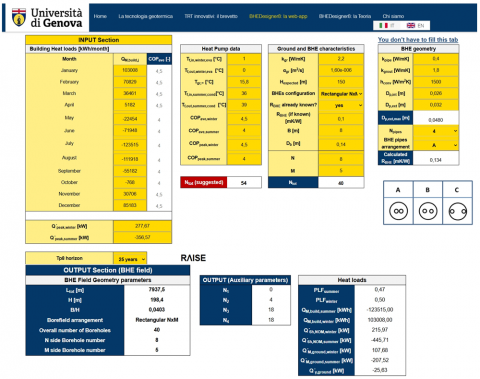
The algorithm of the ASHRAE-Tp 810 and ASHRAE-Tp 825 methods and related equations for the 10 and 25-year horizon designs of BHE fields have been packaged, constituting a comprehensive integrated method accessible as a web application named BHEDesigner8. This tool is available for free use at GeoSensingDesign.org [20]. Figure 1 aims to illustrate the main features of the most updated version of the BHEDesigner8, incorporating the 25-year and the 10-year horizon design methods.
Figure 1. Mask with the main features of the BHEDesigner8 as freely accessible and editable by users
Each user in the world can easily set the input values in the yellow cells of the page and obtain the output values in the blue cells. The algorithm requires inputs (yellow cells) such as the building's monthly heat load, the peak loads in heating and cooling modes, the BHE field configuration, pipes geometry and related diameters, the borehole and ground thermal properties, and the average and the peak values of COP (in heating and cooling) of the heat pump as well as the minimum (or maximum) average (inlet-outlet) fluid temperature Tf,ave(τn) value expected at the end of the considered horizon design method.
The outputs (blue cells) provided by the web tool include the overall length L of the BHEs and their depth (H), the overall number Ntot of BHEs coherent with the related chosen configuration (arrangement of BHEs). The online user can vary in real-time the configuration and related number of boreholes (N and M) along two perpendicular directions.
Worth noticing, the method provides as output the suggested overall number of BHEs to be adopted "Ntot,suggested" (denoted by the Red Cell). In the case the user needs to obtain from the design a borehole depth H close to the expected borehole depth Hexpected (set as input value), the "Ntot,suggested" can be a useful suggested value in order to set the right number of boreholes (N, M, and hence Ntot). The possibility of setting any specific Hexpected is often crucial since its value is closely related and limited by the characteristics of the drilling equipment system available and by geological constraints. The ability to specify the expected BHE depth adds practicality and customization to the design process, allowing users to tailor the BHE field to their specific needs and site conditions, also in terms of drilling space availability. Moreover, the proposed design method, as it has been structured, allows for setting BHE configurations that are not necessarily considered by other commercial codes, provided that the range of B/H is met.
Particular attention has to be given to the new important feature related to the possibility of selecting the 10-year or 25-year horizon design. In addition, the automatic designs by the BHEDesigner8 result from an iterative method that is able to reach convergence very fast, after a few cycles, and in real-time without causing any computation waiting time for the user. These features widely enhance the usability and practicability of the tool, making it a valuable and appealing resource for professionals and engineers of the world in the field of geothermal energy systems (not strictly limited to academic and research experts).
It is important to highlight that, if the borehole thermal resistance Rb is not known (not extrapolated from a TRT), its value can be independently computed within the web app according to the Paul semi-empirical model [21].
Unlike many commercial calculation software tools in the sector, which rely on time superposition/convolution of 12 non-aggregated heat pulses and require an embedded database of pre-computed g-functions, the ASHRAE-Tp 810 and ASHRAE-Tp 825 methods do not need any library of pre-computed g-functions. This is because the corrective temperature penalty Tp is directly reconstructed through Eq. (8) inside the iterative calculation until the convergence on L is achieved. It has to be stressed once more that the constants in Eq. (8) have been preliminarily tuned in comparison with Tp “true” values provided by reference g-functions for a wide range of BHE field configurations. This eliminates the need to evaluate and have available the complete sets of g-functions for deriving the Tp for each specific case, simplifying the calculations and reducing reliance on external databases and computational resources. Additionally, the preliminary tuning of the constants in Eq. (8) ensures accuracy and reliability across various BHE field configurations, including different dimensionless BHE spacings (B/H ratio).
The limitation of the present method is represented by the range of B/H within which the constants of the method itself have been properly tuned and applied. This range, as reported in the previous section, is for 0.03 < B/H < 0.125. BHEDesigner8 informs the user with a dedicated Warning message in case the resulting design is out of this range. A design obtained for a specific B/H out of the range of validity does not necessarily imply that the design is inaccurate or meaningless. It means that the design provided as output could not be reliable since obtained with constants out of the range in which these have been tuned. Thus, the validity of the design obtained is unknown, and the performance set as input in terms of desired COP and expected geothermal carrier fluid temperatures Tf,ave(τn) at the end of the time horizon set (10 or 25-year) could not be guaranteed; the user has to be aware and carefully take into account of the Warning message printed to the screen by the BHEDesigner8 in choosing the right spacing B, N and M to meet the indicated range of B/H.
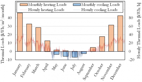
Whereas the main aim of the present section is to give further examples in the comparison of the designs for the 10 and 25-year horizon and arbitrary building heat load profiles could be assumed, a typical North European building structure related to a Swedish multi-family house built in a historical period between 1996-2005, located in Stockholm, has been considered for the present calculations. The building energy needs for heating and cooling and the hourly heat load profiles are obtained from EnergyPlus simulations reported in detail in Fossa et al. [3]. These simulations consider the local climate (as Typical Meteorological Years) and local building envelope characteristics (by the Tabula webtool database).
The monthly building heat loads resulting from EnergyPlus simulations are reported in detail in Figure 2 and are used as input for the BHEs field design tools; these heat loads are estimated by setting the internal temperature of the building to be maintained in the range 20-26℃ all year long. Moreover, based on the hourly EnergyPlus profiles, the peak loads in heating and cooling are estimated according to the approach proposed by Cullin and Spitler [22].
Figure 2. Monthly and hourly building heat loads profiles for a Swedish multi-family house from EnergyPlus
As shown by Figure 2, the Swedish case is characterized by an unbalanced heat load profile (i.e., heating mode largely prevails over the cooling mode) throughout the year; this unbalanced heat load profile acts as the base for further design cases. In fact, a second case of sizing with the ASHRAE-Tp 810 and ASHRAE-Tp 825 methods embedded in the BHEDesigner8 considers a BHE field serving 10 multi-family Swedish houses.
In this manner, the design process is addressed to involve both rectangular and non-rectangular borehole configurations and to highlight how the overall borehole length is highly dependent on the magnitude of the monthly heat loads considered. The same design cases of a BHE field serving 1 and 10 multi-family Swedish houses have been repeated for 3 different kgr (1.5, 3, 6 W/mK) and Rb (0.05, 0.1, 0.2 mK/W) values to have an estimate of how the design is sensitive to variations in the estimated borehole and ground thermal properties.
All these design cases have been performed to guarantee that at the 10th or 25th year of operation both the monthly averaged COPave and the COPpeak are equal to 4.5 in the heating mode (winter season) and 4 in the cooling mode (summer season) of the GCHP. The expected minimum (or maximum) average fluid temperature Tf,ave(τn) corresponding to the assigned COPpeak is set to 0.5℃ in the heating mode (minimum value at the evaporator side of the GCHP) and 37.5℃ in the cooling mode (maximum value at the condenser side of the GCHP).
All these design cases have been performed with both the ASHRAE-Tp 810 and ASHRAE-Tp 825 methods embedded in the BHEDesigner8 and compared with the reference results (REF) provided by EED.
The intrinsic nature of Eq. (1) suggests considering also the important effect of the ratio $\frac{\dot{Q}_h}{\dot{Q}_y}$ between the most demanding hourly heat load $\left(\dot{Q}_h\right)$ and the yearly mean load $\left(\dot{Q}_y\right)$. Considering the same building heat load profile related to 10 multi-family Swedish houses (i.e., at the same $\dot{Q}_y$ and $\dot{Q}_m$), additional cases have been performed by setting different peak loads in order to vary the ratio $\frac{\dot{Q}_h}{\dot{Q}_y}$ (that is always greater than 1 by default). In particular, in some cases, the ratio $\frac{\dot{Q}_h}{\dot{Q}_y}$ has been doubled and halved of the original base case value.
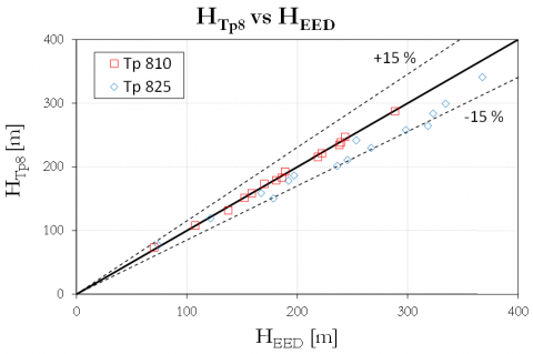
Figure 3 presents the comparison for the single BHE depths H as computed by the reference tool EED (for both the 10- and 25-year time horizon) and the ASHRAE-Tp 810 and ASHRAE-Tp 825 methods. The two sizing approaches consider the same borefield configurations and the comparison in terms of H helps the visualization of all data. The ground volumetric heat capacity has been kept equal to 3 MJ/m3K. The ground thermal conductivity and borehole thermal resistance assume the above-mentioned values. The original values $\dot{Q}_y$ are 7.98 kW and 79.8 kW for 1 and 10 multi-family houses, respectively. The original value of the ratio $\frac{\dot{Q}_h}{\dot{Q}_y}$ is 4.21; some cases having $\dot{Q}_y$ of 79.8 kW have been run with doubled and halved $\frac{\dot{Q}_h}{\dot{Q}_y}$. The values assigned to the borehole spacing for these cases are 8, 8.5, 9.1, and 10.5 m (only for preserving a comparison between EED and Tp8 methods in the range of validity on B/H). The BHE fields considered in the validation are characterized by 4 × 4, 9 × 9, 10 × 12 rectangular, and 1 × 8 in-line (non-RCT) configurations.
Figure 3. Comparison between borehole depths as computed by EED, the ASHRAE-Tp 810 and ASHRAE-Tp 825
Figure 3 shows an excellent agreement with the EED method for the ASHRAE-Tp 810 and a good agreement for the ASHRAE-Tp 825, demonstrating that the proposed one is a sufficiently accurate method to give a reliable design also for the 25-year horizon. As shown by Figure 3, the deviations between EED and ASHRAE-Tp 825 are smaller for smaller borefields (for example, the one for a single multi-family house, i.e., the 4 × 4 rectangular and 1 × 8 in-line configurations); on the contrary, it becomes relevant for larger borefields.
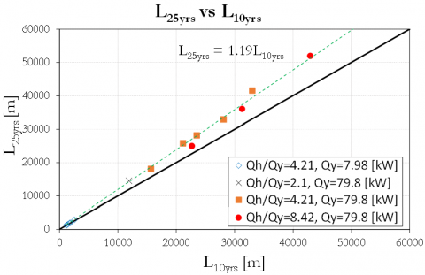
Figure 4 shows the comprehensive comparison between the overall borehole length L as computed by the ASHRAE-Tp 810 and ASHRAE-Tp 825 methods for all the cases covering different $\dot{Q}_y, \frac{\dot{Q}_h}{\dot{Q}_y}$, kgr and Rb. The borehole spacing and the ground volumetric heat capacity have been kept equal to 8 m and 3 MJ/m3K, respectively, for all the cases reported in Figures 4-10.
The impact of different kgr and Rb on the design obtained with the ASHRAE-Tp 810 and ASHRAE-Tp 825 methods is separately detailed in Figures 5-10.
Figure 4. Comparison between overall borehole lengths as computed by the ASHRAE-Tp 810 and ASHRAE-Tp 825
As shown by Figure 4, the increase in the overall borehole length evaluated at the 25th year is included between 3% and 26% (the average increase, including all the cases, is 14%). The lower increments are for cases with $\dot{Q}_y$ quite close to 0 kW (7.98 kW), which is typical for balanced building heat load profiles along the year (the design cases involving the BHE field for a single multi-family house, i.e., the 4 × 4 rectangular and 1 × 8 in-line configurations); notice that when $\dot{Q}_y$ is quite close to 0 kW, consequently Tp is also close to zero according to its definition.
As shown by Figure 4, the deviations between the evaluated overall borehole lengths in the two design horizons become quite considerable when $\dot{Q}_y$ far from 0 kW (the design cases involving the BHE field serving 10 multi-family houses, i.e., the 11 × 13, 12 × 13, 14 × 14 rectangular configurations).
This would demonstrate that the design not only depends on the shape of the building heat load profile (balanced or unbalanced) and the related ratio between the yearly, monthly and hourly heat loads (at the ground side) but, more in general, it strongly depends on the magnitude of $\dot{Q}_y$ which assumes a primary key role in determining L and its increment when evaluated in the 25th year instead of in the 10th year. The $\dot{Q}_y$ far from 0 kW (for example, 79.8 kW) implies that it is comparable to $\dot{Q}_m$ because the heating or cooling loads prevail during the year (the cases with the $\dot{Q}_y$ of 79.8 kW have the $\dot{Q}_m$ of 289.8 kW).
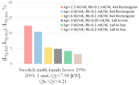
Figure 5. Percentage deviations in overall borehole lengths between the ASHRAE-Tp 810 and ASHRAE-Tp 825 (1 unit)
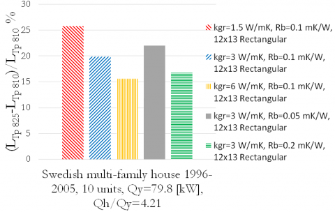
Figure 6. Percentage deviations in overall borehole lengths between the ASHRAE-Tp 810 and ASHRAE-Tp 825 (10 units)
More consistent or attenuated deviations between L25yrs and the L10yrs, at the same $\dot{Q}_y$, are due to variations in kgr, in Rb and in the $\frac{\dot{Q}_h}{\dot{Q}_y}$ ratio. Figures 5 and 6 represent the effects of kgr and of Rb for different magnitudes of $\dot{Q}_y$, at the same $\frac{\dot{Q}_h}{\dot{Q}_y}$ ratio. For both considered $\dot{Q}_y$ values, increasing the ground thermal conductivity significantly reduces the deviations between L25yrs and L10yrs, as suggested by Eqs. (1)-(5). Variations of Rb, similarly to kgr, considerably impact both the time horizon designs. Variations of Rb, differently to kgr, tend not to modify the level of increment in L when evaluated in the 25th year instead of in the 10th year; the spread between the evaluated overall borehole lengths in the two design horizons tends to remain largely unchanged by varying Rb.
The figures also confirm that, as one could expect, $\dot{Q}_y$ far from 0 kW tends to increase and make more remarkable the percentage deviation between the L25yrs and L10yrs, provided the $\frac{\dot{Q}_h}{\dot{Q}_y}$ ratio is not particularly high. Doubling the $\frac{\dot{Q}_h}{\dot{Q}_y}$ ratio, at the same $\dot{Q}_y$, tends to decrease the percentage deviation by about 5% (compare Figures 6 and 7 with the corresponding kgr), independently of the value assumed by B/H. This is particularly true and even potentiated by higher values of kgr, even when $\dot{Q}_y$ is far from 0 kW, as confirmed by Figure 7.
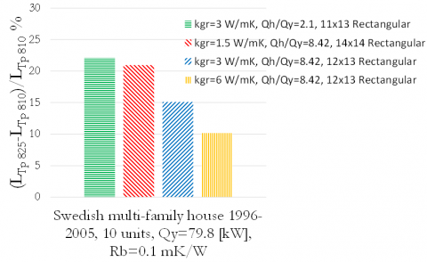
Figure 7. Percentage deviations in overall borehole lengths between the ASHRAE-Tp 810 and ASHRAE-Tp 825 (different kgr and $\frac{\dot{Q}_h}{\dot{Q}_y}$ at the same Rb and $\dot{Q}_y$)
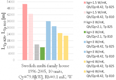
Figure 8 collects and compares the absolute overall borehole lengths at 10 and 25-year horizons obtained by setting the three different kgr values and the same Rb, $\frac{\dot{Q}_h}{\dot{Q}_y}$, and $\dot{Q}_y$ (10 multi-family houses). Figure 9 has the same meaning focusing on the cases for which the $\frac{\dot{Q}_h}{\dot{Q}_y}$ has been varied assuming the three different values. Figure 10 is related to the case of 1 multi-family house unit and reports the same information as Figure 8.
Figure 8. Overall borehole lengths at 10 and 25-year horizons (different kgr at the same Rb, $\frac{\dot{Q}_h}{\dot{Q}_y}$, and $\dot{Q}_y$)
Figure 9. Overall borehole lengths at 10 and 25 years for different kgr and $\frac{\dot{Q}_h}{\dot{Q}_y}$ at the same Rb, and $\dot{Q}_y$ (10 units)
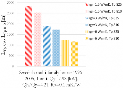
Figure 10. Overall borehole lengths at 10 and 25 years for different kgr at the same Rb, $\frac{\dot{Q}_h}{\dot{Q}_y}$, and $\dot{Q}_y$ (1 unit)
Figures 8-10 highlight once more how strong can be the impact of the ground thermal conductivity and how its correct estimation is crucial on the design of the BHE field. For this reason, the correct preliminary estimation via TRT assumes a key role. Overall, Figures 8-10 show how doubling the values of kgr, at the same $\frac{\dot{Q}_h}{\dot{Q}_y}$ ratio, tends to decrease the absolute overall borehole lengths evaluated at the 10 and 25-year horizon designs and the related percentage deviation between the two horizon designs by about 5%.
The authors make available a powerful and robust web tool named BHEDesigner8, freely accessible and editable online by users for the design of GCHP systems at 10 and 25-year horizons. The main features characterizing the present tool have been accurately described in the present paper. The BHEDesigner8 web application has been efficiently employed to provide a comprehensive comparison between the overall borehole length as computed by the ASHRAE-Tp 810 and ASHRAE-Tp 825 methods for cases covering different $\dot{Q}_y$, $\frac{\dot{Q}_h}{\dot{Q}_y}$, kgr and Rb. The impact of these parameters on the BHE design has been evaluated. In summary, the main conclusions are:
This research is a part of the Italian National Program PNRR - Raise PNRR - ECS00000035 “RAISE (Robotics and AI for Socio economic Empowerment)” - SPOKE 3 “Environmental Caring and Protection Technologies, towards a Zero Emission Environment” - Research Activity (Task) 3.2 “Technologies for energy storage”, CUP D33C22000970006.
|
B |
BHE spacing, m |
|
COP |
Coefficient of Performance related to the heat pump |
|
D |
BHE diameter, m |
|
ΔГ |
deviation between the ICS solution at the time τn and the “true” value related to the exact g-function exponential integral in ILS model |
|
E1 |
Fourier number |
|
Fo |
temperature transfer function in ICS model |
|
G |
dimensionless (multi-BHE) temperature transfer |
|
g |
function |
|
H |
single BHE depth, m |
|
k |
thermal conductivity, W·m⁻¹·K⁻¹ |
|
L |
overall BHEs length, m |
|
M |
number of boreholes in a given direction of the BHE field |
|
N |
number of boreholes in the direction perpendicular to M one |
|
Nj |
number of boreholes with other j at the side of it (j = 1 to 4) |
|
$\dot{Q}$ |
heat transfer rate, W |
|
$\dot{Q}^{\prime}$ |
heat transfer rate per unit length, W·m⁻¹ |
|
r |
radial distance/radius, m |
|
R |
thermal resistance, mK·W⁻¹, spacing of a regular matrix arrangement comprised of 8 BHEs around the central one, m |
|
T |
temperature, ℃ |
|
Tp |
temperature penalty, ℃ |
|
Greek symbols |
|
|
$\alpha$ |
thermal diffusivity, m2·s-1 |
|
π |
pi constant |
|
$\tau$ |
time, s |
|
θ8 |
excess temperature, Eq. (7), °C |
|
Subscripts |
|
|
ave |
average value |
|
b |
borehole |
|
f |
fluid |
|
gr |
ground |
|
h |
referred to 6 hours |
|
m |
referred to 1 month |
|
n |
referred to 10/25 years + 1 month + 6 hours |
|
peak |
referred to the peak heat load at the building side |
|
ref |
reference length (100 m) |
|
tot |
total number of BHEs |
|
p810 |
referred to the Tp8 method related to 10-year horizon |
|
p825 |
referred to the Tp8 method related to 25-year horizon |
|
y |
referred to 10/25 years |
|
∞ |
undisturbed and initial condition |
[1] Kavanaugh, S.P., Rafferty, K. (1997). Ground-source heat pumps: Design of geothermal systems for commercial and institutional buildings. In ASHRAE, Atlanta, Georgia.
[2] Ingersoll, L.R., Zobel, O.J., Ingersoll, A.C. (1954). Heat Conduction with Engineering, Geological, and Other Applications. McGraw-Hill, New York.
[3] Fossa, M., Morchio, S., Priarone, A., Memme, S. (2023). Accurate design of BHE fields for geothermal heat pump systems: The ASHRAE-Tp8 method compared to non aggregated schemes applied to different European test cases. Energy and Buildings, 303: 113814. https://doi.org/10.1016/j.enbuild.2023.113814
[4] Eskilson, P. (1987). Thermal analysis of heat extraction boreholes. Ph.D. thesis, Lund University of Technology.
[5] Ahmadfard, M., Bernier, M. (2018). Modifications to ASHRAE’s sizing method for vertical ground heat exchangers. Science and Technology for the Built Environment, 24: 803-817. https://doi.org/10.1080/23744731.2018.1423816
[6] Kurevija, T., Vulin, D., Krapec, V. (2012). Effect of borehole array geometry and thermal interferences on ground source heat pump system. Energy Conversion and Management, 60: 134-142. https://doi.org/10.1016/j.enconman.2012.02.012
[7] Brown, C.S., Kolo, I., Banks, D., Falcone, G. (2024). Comparison of the thermal and hydraulic performance of single U-tube, double U-tube and coaxial medium-to-deep borehole heat exchangers. Geothermics, 117: 102888. https://doi.org/10.1016/j.geothermics.2023.102888
[8] Heim, E., Stoffel, P., Düber, S., Knapp, D., Kümpel, A., Müller, D., Klitzsch, N. (2024). Comparison of simulation tools for optimizing borehole heat exchanger field operation. Geothermal Energy, 12: 24. https://doi.org/10.1186/s40517-024-00303-8
[9] Blanke, T., Born, H., Döring, B., Göttsche, J., Herrmann, U., Frisch, J., van Treeck, C. (2024). Model for dimensioning borehole heat exchanger applied to mixed-integer-linear-problem (MILP) energy system optimization. Geothermal Energy, 12: 30. https://doi.org/10.1186/s40517-024-00301-w
[10] Magdic, L., Zakula, T., Boban, L. (2023). Improved analysis of borehole heat exchanger performance. Energies, 16(17): 6116. https://doi.org/10.3390/en16176116
[11] Morchio, S., Fossa, M., Priarone, A., Memme, S. (2024). Extended version at 25 years of the ASHRAE-Tp8 method for the design of BHE fields operating with geothermal heat pumps. Geothermics, 123: 103128, https://doi.org/10.1016/j.geothermics.2024.103128
[12] Morchio, S., Fossa, M., Memme, S., Parenti, M., Priarone, A. (2025). Comparison of 10- and 25-year horizon designs for vertical borehole heat exchangers in geothermal heat pump applications. Geothermics, 132: 103457. https://doi.org/10.1016/j.geothermics.2025.103457
[13] Tarrad, A.H. (2021). Borehole thermal analysis for a closed loop vertical U-tube DX ground heat exchanger. Mathematical Modelling of Engineering Problems, 8(4): 501-509. https://doi.org/10.18280/mmep.080402
[14] Chen, H.H., Tomac, I. (2023). Technical review on coaxial deep borehole heat exchanger. Geomechanics and Geophysics for Geo-Energy and Geo-Resources, 9: 120. https://doi.org/10.1007/s40948-023-00659-4
[15] Spitler, J.D. (2000). GLHEPRO: A design tool for commercial building ground loop heat exchangers. In the 4th International Conference on Heat Pumps in Cold Climates, Aylmer, Quebec, Canada, pp. 1-15. https://www.osti.gov/etdeweb/biblio/20144646.
[16] American Society of Heating, Refrigerating and Air-Conditioning Engineers (ASHRAE). (2015). ASHRAE Handbook – HVAC Applications (I-P edition). Chapter 34. Geothermal energy (TC 6.8, Geothermal Heat Pump and Energy Recovery Applications). ASHRAE, Atlanta, State of Georgia.
[17] Carslaw, H.S., Jaeger, J.C. (1959). Conduction of Heat in Solids, 2nd Edition. Oxford University Press. https://doi.org/10.1007/978-1-4939-2565-0_2
[18] Bernier, M.A. (2006). Closed-loop ground-coupled heat pump systems. ASHRAE Journal, 48(9): 12-25.
[19] Mogensen, P. (1983). Fluid to duct wall heat transfer in duct system heat storages. Document-Swedish Council for Building Research, (16): 652-657.
[20] GeoSensingDesign.org. https://www.geosensingdesign.org/, accessed on Apr. 26, 2025.
[21] Paul, N.D. (1996). The effect of grout conductivity on vertical heat exchanger design and performance. Master's thesis, South Dakota State University.
[22] Cullin, J.R., Spitler, J.D. (2011). A computationally efficient hybrid time step methodology for simulation of ground heat exchangers, Geothermics. 40: 144-156. https://doi.org/10.1016/j.geothermics.2011.01.001