S Shenbaga Devi![]() | S Dhanalakshmi*
| S Dhanalakshmi*![]()
© 2025 The authors. This article is published by IIETA and is licensed under the CC BY 4.0 license (http://creativecommons.org/licenses/by/4.0/).
OPEN ACCESS
Topological indices serve to mathematically represent molecular structures, facilitating the analysis of drug effectiveness and improving the drug development process. In this paper, nine topological indices of eight drugs which are calculated and utilized in the management of hypertension during pregnancy. We conduct a Quantitative Structure–Property Relationship (QSPR) study to explore the potential of generalized degree-based indices through the application of linear regression models. The purpose of this study is to assess how well different topological indices, such as ABC(G), M1(G), M2(G), and others, predict important characteristics like boiling point, flash point, molar refractivity, polarizability, and molar volume. The significance and dependability of the findings were guaranteed by the use of statistical measures like the correlation coefficient (r), F-statistic, and p-value to evaluate model performance. The results shed light on how well degree-based indices predict molecular properties and could be helpful for cheminformatics and pharmaceutical modeling. This research enhances the drug development process by utilizing computational techniques and mathematical modeling for increased efficiency and cost-effectiveness.
topological indices, hypertension, degree-based topological indices, physicochemical properties, regression analysis
Hypertension is another name for high blood pressure. Hypertension during pregnancy does not cause signs or symptoms, but leads to problems for both mother and baby. During pregnancy, there are two types of elevated blood pressure that can occur. Chronic hypertension and gestational hypertension are the two types. Prior to becoming pregnant or before 20 weeks of pregnancy, a woman may already have chronic hypertension. Only expectant mothers can expect in gestational hypertension over 20 weeks of pregnancy, which is elevated blood pressure that often goes away after childbirth. However, some women experience high hypertension, which puts them at risk for preeclampsia and other more serious issues later in the pregnancy. Pregnancy – related hypertension can occur for a few different reasons. The volume of blood in a woman’s body can grow by up to 45% while she is pregnant. The heart has to pump this excess blood around the body. The left ventricle grows thicker and larger as a result of substantial pumping. The heart can pump more blood at a faster rate because of this momentary effect. Vasopressin, a hormone that promotes higher water retention, is released in greater quantities by the kidneys. A 10% global prevalence of pregnancy-related hypertension problems is seen. 3%–5% of pregnancy cases result in preeclampsia. It has estimated that 8–10% of women who are pregnant in India develop preeclampsia. According to a study, preeclampsia afflicted 5.4% of India's sample population, and 7.8% of pregnancies were associated with hypertension disorders. Antihypertensive drugs are the mainstay of treatment throughout the first nine months of pregnancy. These drugs are primarily used to prevent and treat severe hypertension, prolong pregnancy as long as it’s safe to do so, and reduce the amount of medicine that the fetus is exposed to. Mathematical modeling provides a quantitative method for early prediction and study of pregnancy induced hypertension by linking clinical parameters with observed outcomes. For further details see the references [1-3].
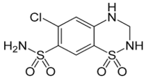
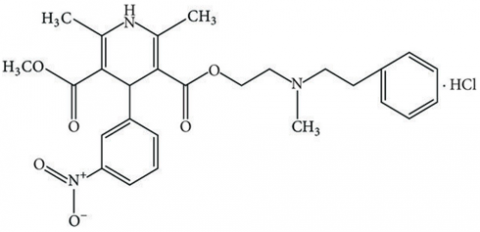
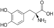
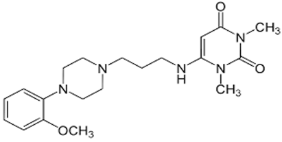
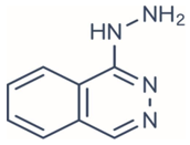
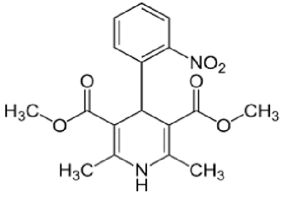
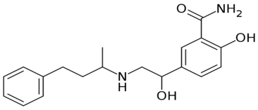
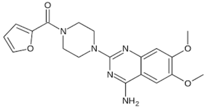
Few antihypertensive drugs like hydrochlorothiazide, nicardipine, methyldopa, urapidil, hydralazine, nifedipine, labetalol, prazosin is identified for the treatment. The drug structures are depicted in Figure 1. The molecular formula for Hydrochlorothiazide is $\mathrm{C}_7 \mathrm{H}_8 \mathrm{CIN}_3 \mathrm{O}_4 \mathrm{S}_2$. Only if the benefits outweigh the risks to the fetus can this be used during pregnancy. The molecular formula for nicardipine is $\mathrm{C}_{26} \mathrm{H}_{29} \mathrm{N}_3 \mathrm{O}_6$. It reduces blood pressure rapidly and effectively during pregnancy. The molecular formula of methyldopa is $\mathrm{C}_{10} \mathrm{H}_{13} \mathrm{NO}_4$. Methyldopa avoids difficulties including preterm birth, low birth weight, and potentially serious illness for both the mother and the child. The molecular formula of Urapidil is $\mathrm{C}_{20} \mathrm{H}_{29} \mathrm{N}_5 \mathrm{O}_3$. Treatment with urapidil was effective to reduce the blood pressure which was higher than 160/110 mmHg to 150/100 mmHg or below. The molecular formulas of Hydralazine are $\mathrm{C}_8 \mathrm{H}_8 \mathrm{N}_4$, Labetalol is $\mathrm{C}_{19} \mathrm{H}_{24} \mathrm{N}_2 \mathrm{O}_3$ and Nifedipine is $\mathrm{C}_{17} \mathrm{H}_{18} \mathrm{N}_2 \mathrm{O}_6$. When a pregnant woman has severe hypertension, she may need an emergency caesarean section and frequently takes magnesium sulphate. Hydralazine, Labetalol, and nifedipine are frequently used to treat this condition. The molecular formula of Prazosin is $\mathrm{C}_{19} \mathrm{H}_{21} \mathrm{N}_5 \mathrm{O}_4$. During the last trimester, prazosin is a safe and effective blood pressure medication.
Graph theory is a mathematics discipline addressing point networks connected via lines. Recreational arithmetic puzzles served as the inspiration for graph theory, but it has evolved into a substantial area of mathematical research, having applications in chemistry. These days, a complete image of molecular structures is provided by molecular topology, graph theory, and physical-chemical measurements like electronic density, melting and boiling points, and ionic and covalent potentials. Moreover, by simulating toxicants, molecular topology by chemical graph theory seems to explain biological activity [4, 5]. The molecular descriptor is the outcome of logical reasoning and mathematical procedure that transforms chemical data stored in a molecule's symbolic representation into a useful component or the result of specific standardized tests. Topological indices attract attention because they correspond strongly with specific chemical features of molecular graphs. Topological indices based on degree can facilitate the prediction of a compound's properties, eliminating the necessity for extensive experimental testing. Traditionally, determining the properties requires extensive laboratory experimentation, which can be time-consuming, costly, and resource-intensive. To address these challenges, Quantitative Structure–Property Relationship (QSPR) models have emerged as effective tools. QSPR methods aim to correlate the structural attributes of molecules with their physicochemical or biological properties, enabling the prediction of unknown properties using computational techniques. This has the potential to optimize efficiency and conserve resources in fields such as pharmaceuticals, ecological research, and materials development. Topological indices grounded in degree can facilitate the exploration of the anti-inflammatory properties within specific chemical networks. Chemistry uses QSPR models to forecast a chemical compound's characteristics based on its molecular structure.
The computation of many degree-based topological indices is part of this study related to medications associated with pregnancy-related hypertension and we have given the theorem proof for the drug Hydrochlorothiazide whereas for the remaining drugs can be generated in the same way. We have also shown how the indices and the chemical structures’ physical characteristics are related using linear regression model [6-9]. Although numerous studies have applied individual topological indices for predicting isolated properties, there is a lack of comparative assessments that systematically evaluate multiple indices across several physicochemical properties. This study addresses that gap by computing and analyzing the correlation of nine different topological indices with five key properties. By doing so, we aim to identify which indices are most suitable for specific property predictions and provide guidance for future QSPR modeling efforts. Additionally, we incorporate detailed calculations [10-12] and internal validation to enhance the interpretability and reliability of the results.
This paper sets itself apart by offering a multi-property, comparative evaluation of topological indices in a consistent QSPR framework. This also assesses and ranks index performance across boiling point, flash point, molar refractivity, polarizability, and molar volume, in contrast to previous studies that concentrated on individual properties or indices. It provides recommendations for index selection in property-specific prediction tasks and lays the groundwork for additional model automation and improvement through this integrative approach. As the foundation for the computation of the topological index, Figure 1 displays the molecular graph representations of the chosen drugs. We have used Chemspider for validating the molecular graphs from the molecular structures.
(a) Hydrochlorothiazide
(b) Nicardipine
(c) Methyldopa
(d) Urapidil
(e) Hydralazine
(f) Nifedipine
(g) Labetalol
(h) Prazosin
Figure 1. Drugs’ molecular structure
The fundamental definitions of the topological indices based on degree were employed are examined in the study in this section:
The definition of a molecular graph G’s ABC index [13] is:
$A B C(G)=\sum_{p q \in E(G)} \sqrt{\frac{d_p+d_q-2}{d_p d_q}}$ (1)
The definition of a molecular graph G’s first Zagreb index [14] is:
$M_1(G)=\sum_{p \in V(G)} d^2(p)$ (2)
The definition of a molecular graph G’s second Zagreb index [15] is:
$M_2(G)=\sum_{p q \in E(G)} d_p d_q$ (3)
The definition of a molecular graph G’s reciprocal Randic index [16] is:
$R R(G)=\sum_{p q \in E(G)} \sqrt{d_p d_q}$ (4)
The definition of a molecular graph G’s hyper-Zagreb index [17] is:
$H M(G)=\sum_{p q \in E(G)}\left(d_p+d_q\right)^2$ (5)
The definition of a molecular graph G’s forgotten index [17] is:
$F(G)=\sum_{p q \in E(G)}\left[d_p^2+d_q^2\right]$ (6)
The definition of a molecular graph G’s Sombor index [18] is:
$S O(G)=\sum_{p q \in E(G)} \sqrt{d_p^2+d_q^2}$ (7)
The definition of a molecular graph G’s inverse sum Indeg index [19] is:
$I S I(G)=\sum_{p q \in E(G)} \frac{d_p d_q}{d_p+d_q}$ (8)
The definition of a molecular graph G’s Shilpa-Shanmukha (SS) index [20] is
$S S(G)=\sum_{p q \in E(G)} \sqrt{\frac{d_p d_q}{d_p+d_q}}$ (9)
This study employed the mentioned nine topological indices to model five physical features: boiling point (BP), molar volume (MV), polarizability (P), flash point (FP), and molar refractivity (MR) of 8 drugs: hydrochlorothiazide, nicardipine, urapidil, hydralazine, nifedipine, labetalol, prazosin, methyldopa. The physicochemical characteristics of the eight medications are shown in Table 1.
Table 1. Physicochemical properties of hypertension drugs in treatment during pregnancy
|
Name of the Medicine |
Boiling Point |
Flash Point |
Molar Refractivity |
Polarizability |
Molar Volume |
|
Hydrochlorothiazide |
577 |
302.7 |
62.7 |
24.9 |
175.8 |
|
Nicardipine |
603.4 |
318.7 |
130 |
51.5 |
389.8 |
|
Urapidil |
549 |
285.8 |
108.3 |
42.9 |
307.4 |
|
Hydralazine |
491.9 |
251.3 |
48.8 |
19.3 |
116.6 |
|
Nifedipine |
475.3 |
241.2 |
87.9 |
34.8 |
272.3 |
|
Labetol |
552.7 |
288.1 |
94.7 |
37.6 |
273.6 |
|
Prazosin |
638.4 |
339.9 |
103.6 |
41.1 |
283.4 |
|
Methyldopa |
441.6 |
220.9 |
53.9 |
21.4 |
150.5 |
3.1 Computation of topological indices
Let $G_1$ represent the hydrochlorothiazide graph. The following are some of its topological indices:
(1) $A B C\left(G_1\right)=13.43$
(2) $M_1\left(G_1\right)=94$
(3) $M_2\left(G_1\right)=111$
(4) $R R\left(G_1\right)=43.74$
(5) $H M\left(G_1\right)=504$
(6) $F\left(G_1\right)=282$
(7) $\operatorname{SO}\left(G_1\right)=70.42$
(8) $I S I\left(G_1\right)=20.51$
(9) $S S\left(G_1\right)=19.04$
Proof: Let $G_1$ represent the hydrochlorothiazide graph. The edges that connect the vertices of degrees $d_p$ and $d_q$ are denoted as $E_{(p, q)}$. Table 2 illustrates the edge set partition of $G_1$.
Table 2. Partition of edges
|
E[dp, dq] |
E(1,4) |
E(1,3) |
E(2,3) |
E(2,2) |
E(3,3) |
E(3,4) |
E(2,4) |
|
Number of edges |
5 |
1 |
5 |
2 |
2 |
2 |
1 |
(1) The following is obtained by utilizing Table 2 and Eq. (1):
$A B C\left(G_1\right)=5 \sqrt{\frac{1+4-2}{1 \times 4}}+1 \sqrt{\frac{1+3-2}{1 \times 3}}+5 \sqrt{\frac{2+3-2}{2 \times 3}}+2 \sqrt{\frac{2+2-2}{2 \times 2}}+2 \sqrt{\frac{3+3-2}{3 \times 3}}+2 \sqrt{\frac{3+4-2}{3 \times 4}}+1 \sqrt{\frac{2+4-2}{2 \times 4}}=13.43$.
(2) The following is obtained by utilizing Table 2 and Eq. (2):
$M_1\left(G_1\right)=5(1+4)+1(1+3)+5(2+3)+2(2+2)+2(3+3)+2(3+4)+1(2+4)=94$.
(3) The following is obtained by utilizing Table 2 and Eq. (3):
$M_2\left(G_1\right)=5(1 \times 4)+1(1 \times 3)+5(2 \times 3)+2(2 \times 2)+2(3 \times 3)+2(3 \times 4)+1(2 \times 4)=111$.
(4) The following is obtained by utilizing Table 2 and Eq. (4):
$R R\left(G_1\right)=5 \sqrt{1 \times 4}+1 \sqrt{1 \times 3}+5 \sqrt{2 \times 3}+2 \sqrt{2 \times 2}+2 \sqrt{3 \times 3}+2 \sqrt{3 \times 4}+1 \sqrt{2 \times 4}=43.74$.
(5) The following is obtained by utilizing Table 2 and Eq. (5):
$H M\left(G_1\right)=5(1+4)^2+1(1+3)^2+5(2+3)^2+2(2+2)^2+2(3+3)^2+2(3+4)^2+1(2+4)^2=504$.
(6) The following is obtained by utilizing Table 2 and Eq. (6):
$F\left(G_1\right)=5\left(1^2+4^2\right)+1\left(1^2+3^2\right)+5\left(2^2+3^2\right)+2\left(2^2+2^2\right)+2\left(3^2+3^2\right)+2\left(3^2+4^2\right)+1\left(2^2+4^2\right)=282$.
(7) The following is obtained by utilizing Table 2 and Eq. (7):
$S O\left(G_1\right)=5 \sqrt{1^2+4^2}+1 \sqrt{1^2+3^2}+5 \sqrt{2^2+3^2}+2 \sqrt{2^2+2^2}+2 \sqrt{3^2+3^2}+2 \sqrt{3^2+4^2}+1 \sqrt{2^2+4^2}=70.42$.
(8) The following is obtained by utilizing Table 2 and Eq. (8):
$I S I\left(G_1\right)=5\left(\frac{1 \times 4}{1+4}\right)+1\left(\frac{1 \times 3}{1+3}\right)+5\left(\frac{2 \times 3}{2+3}\right)+2\left(\frac{2 \times 2}{2+2}\right)+2\left(\frac{3 \times 3}{3+3}\right)+2\left(\frac{3 \times 4}{3+4}\right)+1\left(\frac{2 \times 4}{2+4}\right)=20.51$.
(9) The following is obtained by utilizing Table 2 and Eq. (9):
$S S\left(G_1\right)=5 \sqrt{\left(\frac{1 \times 4}{1+4}\right)}+1 \sqrt{\left(\frac{1 \times 3}{1+3}\right)}+5 \sqrt{\left(\frac{2 \times 3}{2+3}\right)}+2 \sqrt{\left(\frac{2 \times 2}{2+2}\right)}+2 \sqrt{\left(\frac{3 \times 3}{3+3}\right)}+2 \sqrt{\left(\frac{3 \times 4}{3+4}\right)}+1 \sqrt{\left(\frac{2 \times 4}{2+4}\right)}=19.04$.
Likewise, the topological indices of the other molecular drugs are calculated and Table 3 shows the outcomes and Figure 2 gives the two-dimensional graph of the topological indices with respect to the drugs.
Table 3. Topological indices of hypertension drugs in treatment during pregnancy
|
Name of the Medicine |
ABC(G) |
M1(G) |
M2(G) |
RR(G) |
HM(G) |
F(G) |
SO(G) |
ISI(G) |
SS(G) |
|
Hydrochlorothiazide |
13.43 |
94 |
111 |
43.74 |
504 |
282 |
70.42 |
20.51 |
19.04 |
|
Nicardipine |
26.61 |
176 |
205 |
85.38 |
862 |
452 |
127.81 |
41.52 |
38.92 |
|
Urapidil |
20.03 |
132 |
153 |
64.42 |
638 |
332 |
95.37 |
31.5 |
29.54 |
|
Hydralazine |
9.11 |
60 |
70 |
29.66 |
286 |
146 |
42.89 |
14.67 |
13.74 |
|
Nifedipine |
17.19 |
116 |
139 |
56.19 |
584 |
306 |
84.34 |
27.28 |
25.33 |
|
Labetol |
18.10 |
116 |
130 |
56.16 |
550 |
290 |
84.39 |
27.25 |
25.96 |
|
Prazosin |
21.9 |
150 |
180 |
73.48 |
746 |
386 |
108.08 |
35.03 |
33.24 |
|
Methyldopa |
11.26 |
74 |
83 |
34.47 |
376 |
210 |
55.47 |
16.15 |
15.42 |
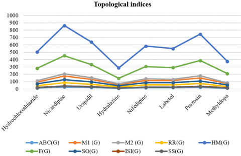
According to Table 3, Nicardipine has the highest values for almost every index, suggesting a complex, highly branched, and potentially stable molecular structure. Hydralazine and methyldopa, on the other hand, have the lowest values, indicating less complex and branched structures. The similarity between nifedipine and labetol suggests that their molecular topologies are similar. These graph-based descriptors can be used to predict molecular behavior, reactivity, or pharmacological properties.
Figure 2. Topological indices with respect to the drugs
Figure 2 clearly shows how the antihypertensive medications under study exhibit notable structural variation, according to the topological indices.
3.2 Model for regression analysis
Regression models are employed to establish a correlation between certain topological indices and the different medications used for managing hypertension in pregnant individuals. The linear regression model is a fundamental statistical technique that assists in identifying the relationship. This model provides significant assistance to individuals in the pharmaceutical industry by uncovering risk factors linked to diseases through the identification of relationships between topological indices, including the ABC index and Randic index, and dependent variables such as boiling point and flash point.
The verification of the linear regression model is conducted through the Eq. (10):
$P=C+b(T I)$ (10)
where, P is the physical property of hypertension drugs during pregnancy, TI represents the topological index, b denotes the regression coefficient, and C signifies a constant.
Based on Eq. (10), the subsequent linear regression models are presented:
(1) Linear regression model for atom bond connectivity index: ABC(G)
$\begin{gathered}\text { Boiling Point }=399.4585+8.2368[A B C(G)] \\ \text { Flash Point }=195.3934+4.9804[A B C(G)] \\ \text { Molar refractivity }=2.0442+4.8939[A B C(G)] \\ \text { Polarizability }=0.8274+1.9391[A B C(G)] \\ \text { Molar Volume }=-18.4881+15.3840[A B C(G)]\end{gathered}$
(2) Linear regression model for first Zagreb index: $M_1$(G)
$\begin{gathered}\text { Boiling Point }=393.9869+1.2826\left[M_1(G)\right] \\ \text { Flash Point }=192.0892+0.7755\left[M_1(G)\right] \\ \text { Molar refractivity }=2.8941+0.7263\left[M_1(G)\right] \\ \text { Polarizability }=1.1635+0.2878\left[M_1(G)\right] \\ \text { Molar Volume }=-15.5784+2.2811\left[M_1(G)\right]\end{gathered}$
(3) Linear regression model for second Zagreb index: $M_2$(G)
$\begin{gathered}\text { Boiling Point }=395.6376+1.0870\left[M_2(G)\right] \\ \text { Flash Point }=193.091+0.6572\left[M_2(G)\right] \\ \text { Molar refractivity }=5.7757+0.6010\left[M_2(G)\right] \\ \text { Polarizability }=2.3082+0.2381\left[M_2(G)\right] \\ \text { Molar Volume }=-6.3178+1.8860\left[M_2(G)\right]\end{gathered}$
(4) Linear regression model for reciprocal Randic index: RR(G)
$\begin{gathered}\text { Boiling Point }=397.7033+2.5878 R R(G) \\ \text { Flash Point }=194.3346+1.5647 R R(G) \\ \text { Molar refractivity }=4.5982+1.4726 R R(G) \\ \text { Polarizability }=1.8416+0.5835 R R(G) \\ \text { Molar Volume }=-9.3787+4.6098 R R(G)\end{gathered}$
(5) Linear regression model for hyper-Zagreb index: HM(G)
$\begin{gathered}\text { Boiling Point }=388.4215+0.2688[H M(G)] \\ \text { Flash Point }=188.7309+0.1625[H M(G)] \\ \text { Molar refractivity }=3.2457+0.1461[H M(G)] \\ \text { Polarizability }=1.2998+0.0579[H M(G)] \\ \text { Molar Volume }=-15.6792+0.4608[H M(G)]\end{gathered}$
(6) Linear regression model for forgotten index: F(G)
$\begin{gathered}\text { Boiling Point }=383.5375+0.5245[F(G)] \\ \text { Flash Point }=185.7810+0.3171[F(G)] \\ \text { Molar refractivity }=2.0391+0.2802[F(G)] \\ \text { Polarizability }=0.8157+0.1111[F(G)] \\ \text { Molar Volume }=-20.9209+0.8888[F(G)]\end{gathered}$
(7) Linear regression model for Sombor index: SO(G)
$\begin{gathered}\text { Boiling Point }=391.4773+1.7906[S O(G)] \\ \text { Flash Point }=190.5731+1.0826[S O(G)] \\ \text { Molar refractivity }=1.7683+1.0104[S O(G)] \\ \text { Polarizability }=0.7149+0.4004[S O(G)] \\ \text { Molar Volume }=-19.852+3.1823[S O(G)]\end{gathered}$
(8) Linear regression model for inverse sum Indeg index: ISI(G)
$\begin{gathered}\text { Boiling Point }=402+5.2045[I S(G)] \\ \text { Flash Point }=196.9328+3.1468[I S(G)] \\ \text { Molar refractivity }=5.1026+3.0344[I S(G)] \\ \text { Polarizability }=2.0453+1.2021[I S(G)] \\ \text { Molar Volume }=-7.8317+9.4996[I S(G)]\end{gathered}$
(9) Linear regression model for Shilpa-Shanmukha index: SS(G)
$\begin{gathered}\text { Boiling Point }=401.3118+5.5609[S S(G)] \\ \text { Flash Point }=196.5138+3.3624[S S(G)] \\ \text { Molar refractivity }=5.1242+3.2253[S S(G)] \\ \text { Polarizability }=2.0515+1.2778[S S(G)] \\ \text { Molar Volume }=-7.2681+10.0778[S S(G)]\end{gathered}$
Table 4. Coefficient of correlation between the drug Ti’s and physicochemical characteristics
|
Topological Index |
BP |
FP |
MR |
PR |
MV |
|
ABC(G) |
0.7107 |
0.7106 |
0.9856 |
0.9859 |
0.9772 |
|
M1(G) |
0.7366 |
0.7365 |
0.9736 |
0.9738 |
0.9644 |
|
M2(G) |
0.7449 |
0.7448 |
0.9613 |
0.9615 |
0.9515 |
|
RR(G) |
0.7357 |
0.7356 |
0,9772 |
0,9774 |
0.9648 |
|
HM(G) |
0.7484 |
0.7482 |
0.9492 |
0.9495 |
0.9446 |
|
F(G) |
0.7467 |
0.7465 |
0.931 |
0.9315 |
0.9315 |
|
SO(G) |
0.7357 |
0.7356 |
0.9691 |
0.9694 |
0.9626 |
|
ISI(G) |
0.7227 |
0.7227 |
0.9834 |
0.9835 |
0.9711 |
|
SS(G) |
0.7264 |
0.7263 |
0.9834 |
0.9835 |
0.9711 |
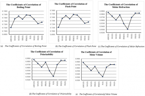
Table 4 shows, there is a strong predictive relationship between topological indices and physicochemical properties, particularly with regard to molar refractivity (MR), polarizability (PR), and molar volume (MV), where correlation values exceed 0.96 for the majority of indices. Structural descriptors appear to be reasonably effective in modeling thermal behavior, as evidenced by their moderate correlations with boiling point (BP) and flash point (FP). The indices that exhibit the strongest overall correlations with the properties under study are $A B C(G), M_1(G), I S I(G) \& S S(G)$, suggesting that they may be useful in QSAR/QSPR modeling. Figure 3 shows the coefficients of correlation of each of the physicochemical property with respect to the topological indices.
Figure 3. The coefficients of correlation of physicochemical properties with topological indices
3.3 Indicators of statistical significance for the linear QSPR model of the topological characteristics
From Tables 5-8, all five properties have p-values less than 0.05, which suggests that the relationships are statistically significant. Strong model fit is demonstrated by the high r values and F-values for polarizability and molar refraction.
Table 5. Statistical parameters for the linear QSPR model for ABC(G)
|
Physical Property |
N |
A |
b |
r |
r2 |
F |
p |
Indicator |
|
Boiling point |
8 |
399.4585 |
8.2368 |
0.7107 |
0.5051 |
6.1237 |
0.0482 |
significant |
|
Flash point |
8 |
195.3934 |
4.9804 |
0.7106 |
0.505 |
6.1212 |
0.0482 |
significant |
|
Molar refraction |
8 |
2.0442 |
4.8939 |
0.9856 |
0.9714 |
203.7902 |
0.0000 |
significant |
|
Polarizability |
8 |
0.8274 |
1.9391 |
0.9859 |
0.972 |
208.2857 |
0.0000 |
significant |
|
Molar volume |
8 |
-18.4881 |
15.3840 |
0.9772 |
0.9549 |
127.0377 |
0.0000 |
significant |
Table 6. Statistical parameters for the linear QSPR model for M1(G)
|
Physical Property |
N |
A |
b |
r |
r2 |
F |
p |
Indicator |
|
Boiling point |
8 |
393.9869 |
1.2826 |
0.7366 |
0.5426 |
7.1176 |
0.0371 |
significant |
|
Flash point |
8 |
192.0892 |
0.7755 |
0.7365 |
0.5424 |
7.1119 |
0.0372 |
significant |
|
Molar refraction |
8 |
2.8941 |
0.7263 |
0.9736 |
0.9479 |
109.1631 |
0.0000 |
significant |
|
Polarizability |
8 |
1.1635 |
0.2878 |
0.9738 |
0.9483 |
110.0542 |
0.0000 |
significant |
|
Molar volume |
8 |
-15.5784 |
2.2811 |
0.9644 |
0.9301 |
79.8369 |
0.0001 |
significant |
Table 7. Statistical parameters for the linear QSPR model for M2(G)
|
Physical Property |
N |
A |
b |
r |
r2 |
F |
p |
Indicator |
|
Boiling point |
8 |
395.6376 |
1.0870 |
0.7449 |
0.5549 |
7.4801 |
0.034 |
significant |
|
Flash point |
8 |
193.091 |
0.6572 |
0.7448 |
0.5547 |
7.4741 |
0.034 |
significant |
|
Molar refraction |
8 |
5.7757 |
0.6010 |
0.9613 |
0.9241 |
73.0514 |
0.0001 |
significant |
|
Polarizability |
8 |
2.3082 |
0.2381 |
0.9615 |
0.9245 |
73.4702 |
0.0001 |
significant |
|
Molar volume |
8 |
-6.3178 |
1.8860 |
0.9515 |
0.9054 |
57.4249 |
0.0003 |
significant |
Table 8. Statistical parameters for the linear QSPR model for RR(G)
|
Physical Property |
N |
A |
b |
r |
r2 |
F |
p |
Indicator |
|
Boiling point |
8 |
397.7033 |
2.5878 |
0.7357 |
0.5413 |
7.0804 |
0.0375 |
significant |
|
Flash point |
8 |
194.3346 |
1.5647 |
0.7356 |
0.5411 |
7.0747 |
0.0375 |
significant |
|
Molar refraction |
8 |
4.5982 |
1.4726 |
0.9772 |
0.9549 |
127.0377 |
0.0000 |
significant |
|
Polarizability |
8 |
1.8416 |
0.5835 |
0.9774 |
0.9553 |
128.2282 |
0.0000 |
significant |
|
Molar volume |
8 |
-9.3787 |
4.6098 |
0.9648 |
0.9308 |
80.7052 |
0.0001 |
significant |
Table 9. Statistical parameters for the linear QSPR model for HM(G)
|
Physical Property |
N |
A |
b |
r |
r2 |
F |
p |
Indicator |
|
Boiling point |
8 |
388.4251 |
0.2688 |
0.7484 |
0.5601 |
7.6395 |
0.0327 |
significant |
|
Flash point |
8 |
188.7309 |
0.1625 |
0.7482 |
0.5598 |
7.6302 |
0.0328 |
significant |
|
Molar refraction |
8 |
3.2457 |
0.1461 |
0.9492 |
0.901 |
54.6061 |
0.0003 |
significant |
|
Polarizability |
8 |
1.2998 |
0.0579 |
0.9495 |
0.9016 |
54.9756 |
0.0003 |
significant |
|
Molar volume |
8 |
-15.6792 |
0.4608 |
0.9446 |
0.8923 |
49.7103 |
0.0004 |
significant |
Table 10. Statistical parameters for the linear QSPR model for SO(G)
|
Physical Property |
N |
A |
b |
r |
r2 |
F |
p |
Indicator |
|
Boiling point |
8 |
391.4773 |
1.7906 |
0.7357 |
0.5413 |
7.0804 |
0.0375 |
significant |
|
Flash point |
8 |
190.5731 |
1.0826 |
0.7356 |
0.5411 |
7.0747 |
0.0375 |
significant |
|
Molar refraction |
8 |
1.7683 |
1.0104 |
0.9691 |
0.9392 |
92.6842 |
0.0000 |
significant |
|
Polarizability |
8 |
0.7149 |
0.4004 |
0.9694 |
0.9397 |
93.5025 |
0.0001 |
significant |
|
Molar volume |
8 |
-19.852 |
3.1823 |
0.9626 |
0.9266 |
75.7439 |
0.0001 |
significant |
Table 11. Statistical parameters for the linear QSPR model for F(G)
|
Physical Property |
N |
A |
b |
r |
r2 |
F |
p |
Indicator |
|
Boiling point |
8 |
383.5375 |
0.5245 |
0.7467 |
0.5576 |
7.5624 |
0.0333 |
significant |
|
Flash point |
8 |
185.7810 |
0.3171 |
0.7465 |
0.5573 |
7.5532 |
0.0334 |
significant |
|
Molar refraction |
8 |
2.0391 |
0.2802 |
0.931 |
0.8668 |
39.0450 |
0.0008 |
significant |
|
Polarizability |
8 |
0.8157 |
0.1111 |
0.9315 |
0.8677 |
39.3515 |
0.0008 |
significant |
|
Molar volume |
8 |
-20.9209 |
0.8888 |
0.9315 |
0.8677 |
39.3515 |
0.0008 |
significant |
Table 12. Statistical parameters for the linear QSPR model for ISI(G)
|
Physical Property |
N |
A |
b |
r |
r2 |
F |
p |
Indicator |
|
Boiling point |
8 |
402 |
5.2045 |
0.7227 |
0.5223 |
6.5602 |
0.0428 |
significant |
|
Flash point |
8 |
196.9328 |
3.1468 |
0.7227 |
0.5223 |
6.5576 |
0.0429 |
significant |
|
Molar refraction |
8 |
5.1026 |
3.0344 |
0.9834 |
0.9671 |
176.3708 |
0.0000 |
significant |
|
Polarizability |
8 |
2.0453 |
1.2021 |
0.9835 |
0.9673 |
177.4862 |
0.0000 |
significant |
|
Molar volume |
8 |
-7.8317 |
9.4996 |
0.9711 |
0.943 |
201.6125 |
0.0000 |
significant |
Table 13. Statistical parameters for the linear QSPR model for SS(G)
|
Physical Property |
N |
A |
b |
r |
r2 |
F |
p |
Indicator |
|
Boiling point |
8 |
401.3118 |
5.5609 |
0.7264 |
0.5277 |
6.7038 |
0.0413 |
Significant |
|
Flash point |
8 |
196.5138 |
3.3624 |
0.7263 |
0.5275 |
6.6984 |
0.0413 |
Significant |
|
Molar refraction |
8 |
5.1242 |
3.2253 |
0.9834 |
0.9671 |
176.3708 |
0.0000 |
Significant |
|
Polarizability |
8 |
2.0515 |
1.2778 |
0.9835 |
0.9673 |
177.4862 |
0.0000 |
Significant |
|
Molar volume |
8 |
-7.2681 |
10.0778 |
0.9691 |
0.9392 |
188.1748 |
0.0000 |
Significant |
From Tables 9 and 10, all five properties have p-values less than 0.05, which suggests that the relationships are statistically significant. Strong model fit is demonstrated by the high r values and F-values for polarizability and molar refraction.
From Tables 11-13 all five properties have p-values less than 0.05, which suggests that the relationships are statistically significant. Strong model fit is demonstrated by the high r values and F-values for molar volume, polarizability and molar refraction.
3.4 Standard error of the estimate
The standard error (SE) of the sample mean is contingent upon both the standard deviation and the sample size. The standard error is mostly utilized for calculating confidence intervals and assessing statistical significance. It quantifies the accuracy of predictions made concerning the computed regression line, as seen in the Table 14.
Table 14. Standard error of the estimate
|
TI |
SE of BP |
SE of FP |
SE of MR |
SE of PR |
SE of MV |
|
ABC(G) |
50.96057 |
30.81866 |
5.24532 |
2.05980 |
20.88680 |
|
M1(G) |
48.99659 |
29.633300 |
7.08948 |
2.79437 |
26.02717 |
|
M2(G) |
48.33020 |
29.23174 |
8.54725 |
3.37826 |
30.28032 |
|
RR(G) |
49.06372 |
29.67296 |
6.58562 |
2.59845 |
25.87194 |
|
HM(G) |
48.04520 |
29.06064 |
9.77009 |
3.85739 |
32.30925 |
|
F(G) |
48.18572 |
29.14664 |
11.33081 |
4.47256 |
35.80146 |
|
SO(G) |
49.06044 |
29.67209 |
7.65532 |
3.01622 |
26.64630 |
|
ISI(G) |
50.07035 |
30.28153 |
5.62635 |
2.22444 |
23.50075 |
|
SS(G) |
49.78620 |
30.10864 |
5.63456 |
2.22292 |
24.26527 |
Table 14 shows that slightly higher standard error values for boiling point indicate more variability in those models, whereas lower standard error values for molar refraction and polarizability indicate highly reliable coefficient estimates.
4.1 Conclusion
This study established topological indices and correlated them with the linear QSPR model for medicines utilized in managing hypertension during pregnancy. The combined mathematical-clinical methodology not only improves our comprehension of medication interactions at the molecular level but also facilitates economical virtual screening in maternal health treatments. The objective of calculating these nine topological indices stems from the fact that a single topological index has not yet been identified that effectively represents all physical properties of the drugs. Gathering information on the structure's topology is the aim of this investigation by utilizing topological indices efficiently and cost-effectively. ABC(G) and SS(G) were more useful for polarizability and molar refractivity, but indices such as M2(G) and HM(G) demonstrated strong correlations with boiling and flash points. The results obtained demonstrate strong correlation coefficients between the physicochemical properties and their corresponding topological indices. The analysis indicates a strong correlation between MR and PR with all the topological indices examined in this study. All these models exhibit a correlation coefficient over 0.7, resulting in a p-value less than or equal to 0.05, hence indicating the relevance of the findings.
4.2 Study implications and future investigations
Utilizing the values of these topological indices, this study provides guidance to chemists and professionals in the pharmaceutical industry in the development of innovative drugs. However, because of dataset limitations, external validation was not possible. The compound library will be extended in future studies to incorporate separate test sets and evaluate generalizability in greater detail. Future studies should enlarge the molecular dataset and incorporate the most promising indices into predictive modeling frameworks in order to convert these correlations into useful tools. Establishing the predictive ability of topological indices in actual compound screening requires these validation procedures. This could help chemists effectively screen compounds for the desired electronic and thermal properties. In alignment with this study, the exploration of different chemical structures is achievable, and insights can be obtained by analysing the relationship between the physical properties of the compounds and the values of the topological indices. A multidisciplinary project can be embraced by individuals from diverse fields to achieve enhanced outcomes.
[1] Kattah, A.G., Garovic, V.D. (2013). The management of hypertension in pregnancy. Advances in Chronic Kidney Disease, 20(3): 229-239. https://doi.org/10.1053/j.ackd.2013.01.014
[2] Podymow, T., August, P. (2008). Update on the use of antihypertensive drugs in pregnancy. Hypertension, 51(4): 960-969. https://doi.org/10.1161/HYPERTENSIONAHA.106.075895
[3] Nirupama, R., Divyashree, S., Janhavi, P., Muthukumar, S.P., et al. (2021). Preeclampsia: Pathophysiology and management. Journal of Gynecology Obstetrics and Human Reproduction, 50(2): 101975. https://doi.org/10.1016/j.jogoh.2020. 101975
[4] Todeschini, R., Consonni, V. (2008). Handbook of Molecular Descriptors. John Wiley Sons. https://onlinelibrary.wiley.com/doi/book/10.1002/9783527613106.
[5] Trinajstic, N. (2018). Chemical Graph Theory. CRC Press, p. 352. https://doi.org/10.1201/97813151 39111
[6] Gutman, I., Trinajstić, N., Wilcox, C.F. (1975). Graph theory and molecular orbitals. XII. Acyclic polyenes. Journal of Chemical Physics, 62(9): 3399-3405. https://doi.org/10.1063/1.430994
[7] Shanmukha, M.C., Usha, A., Praveen, B.M., Douhadji, A. (2022). Degree-based molecular descriptors and QSPR analysis of breast cancer drugs. Journal of Mathematics, 2022(1): 5880011. https://doi.org/10.1155/2022/5880011.
[8] Devi, S.S., Dhanalakshmi, S. (2024). Analysis of degree-based topological indices for stroke treatment drugs: A study on the physicochemical features. IAENG International Journal of Applied Mathematics, 54(6): 1233-1239. https://www.iaeng.org/IJAM/issues_v54/issue_6/index.html.
[9] Adnan, M., Bokhary, S.A. U.H., Abbas, G., Iqbal, T. (2022). Degree-based topological indices and QSPR analysis of antituberculosis drugs. Journal of Chemistry, 2022(1): 5748626. http://doi.org/10.1155/2022/5748626
[10] Movahedi, F., Zameni, M., Akhbari, M.H., Hassan, M., Shahavi, S., Rajabnezhad, S. (2025). Topological indices and data analysis techniques modeling to predict the physicochemical properties of tetracycline antibiotics. Journal of Pharmaceutical Sciences, 114(8): 10387. https://doi.org/10.1016/j.xphs.2025.103871
[11] Isamel, M., Zaman, S., Elahi, K., Koam, A.N.A., Bashir, A. (2024). Analytical expressions and structural characterization of some molecular models through degree based topological indices. Mathematical Modelling of Engineering Problems, 11(1): 47-62. https://doi.org/10.18280/mmep.110105
[12] Ahmed, W.E., Hanif, M.F., Alzahrani, E., Fiidow, O.A. (2025). Predicting bone cancer drugs properties through topological indices and machine learning. Scientific Reports, 15: 31150. https://doi.org/10.1038/s41598-025-16497-1
[13] Das, K.C., Gutman, I., Furtula, B. (2011). On atom-bond connectivity index. Chemical Physics Letters, 511(4-6): 452-454. https://doi.org/10.1016/j.jmaa.2019. 06.069
[14] Gutman, I. (2013). Degree-based topological indices. Croatica Chemica Acta, 86(4): 351-361. http://doi.org/10.5562/cca2294
[15] Gutman, I., Furtula, B., Elphick, C. (2014). Three new/old vertex-degree-based topological indices. Communications in Mathematical and in Computer Chemistry, 72: 617-632. https://match.pmf.kg.ac.rs/electronic_versions/Match72/n3/match72n3_617-632.pdf.
[16] Shirdel, G.H., Rezapour, H., Sayadi, A.M. (2013). The Hyper-Zagreb index of graph operations. Iranian Journal of Mathematical Chemistry, 4: 213-220. https://doi.org/10.22052/ijmc.2013.5294
[17] Furtula, B., Gutman, I. (2015). A forgotten topological index. Journal of Mathematical Chemistry, 53(4): 1184-1190. http://doi.org/10.1007/s10910-015-0480-z
[18] Gutman, I. (2021). Geometric approach to degree-based topological indices: Sombor indices. Communications in Mathematical and in Computer Chemistry, 86(1): 11-16. https://match.pmf.kg.ac.rs/electronic_versions/Match86/n1/match86n1_11-16.pdf.
[19] Vukičević, D., Gašperov, M. (2010). Bond additive modeling 1. Adriatic indices. Croatica Chemica Acta, 83(3): 243-260.
[20] Zhao, W., Shanmukha, M.C., Usha, A., Farahani, M.R., et al. (2021). Computing SS index of certain dendrimers. Journal of Mathematics, 2021(1): 7483508. https://doi.org/10.1155/2021/7483508