Abdulelah Hameed Yaseen*![]() | Yaseen Ahmed Mohammed Alsumaidaee
| Yaseen Ahmed Mohammed Alsumaidaee![]()
© 2025 The authors. This article is published by IIETA and is licensed under the CC BY 4.0 license (http://creativecommons.org/licenses/by/4.0/).
OPEN ACCESS
This study assesses the flow characteristics and resistance in a basic closed hydraulic system commonly found in vehicles. The aim is to determine the total resistances by applying pressure values and flow equations using MATLAB and Simulink. These tools simulate fluid flow through variable orifices, different cross-sections, and turns, considering varying valve positions and loads. We derived formulas to calculate total resistances, including hydraulic and frictional resistances caused by changes in the port's cross-sectional area. We modeled the system's behavior by assessing the valve spool position and experimentally determining that the fluid starts flowing when the valve position is Xv = 0.05 cm. We used various curves to obtain numerical values, with resistances dependent on several parameters. Results indicated that total resistance was highest at this position, with an inverse relationship to Xv. A 20% displacement of the valve spool from 0.05 cm resulted in a 130% reduction in resistance. The resistance also varied with the load on the piston arm, increasing five times for an 8-fold load increase, resulting in a 4.3-fold decrease in flow rate. Additionally, the flow gain factor (k) affected flow characteristics, explaining hydraulic piston slippage under load. The flow coefficient (CV), derived from flow rate and pressure drop, was also crucial in evaluating the valve size specification for the hydraulic system. These findings provide insights into optimizing valve designs and enhancing hydraulic system performance, emphasizing the influence of flow parameters on operational behavior.
hydraulic systems, flow gain, pressure, resistance formulas, flow coefficient, valve optimization, hydraulic resistance, orifice and spool valve
Hydraulic systems have many applications in industries, construction equipment, metal cutting and smelting machines, vehicle steering assemblies, machinery factories, robotics, and others [1, 2] due to their ability to handle large loads because they use pressurized fluids and can maintain high pressures and flow for a longer period of time [3].
In addition to their high durability, their ability to produce large power at high speeds, and their potential to convert the kinetic energy of fluids into mechanical work without the need for auxiliary devices, hydraulic systems are widely used in various industries [4].
The early 20th century saw the rapid development of fluid power technology, primarily due to the introduction of the first generation of hydraulic motors, which primarily accommodated flow controllers. These controllers operated the hydraulic motor in an open-loop manner, facilitating fluid movement by operating the pump, a feature that is commonly used in firefighting and liquid cooling systems [5, 6].
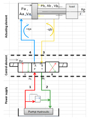
Closed-loop hydraulic systems are characterized by the action of the hydraulic motor, which transfers mechanical energy and/or fluid-assisted motion [7]. The basic elements of closed hydraulic systems consist of a control element (valve) to direct fluid flow, an actuator (power cylinder) that converts hydraulic energy into mechanical work, and a hydraulic power source (pump) that acts as a converter from mechanical work to hydraulic energy. The other components of the system are the tank, safety valves, and overflow [8].
Furthermore, the closed-loop throttle hydraulic drive system works by moving the fluid in a circle and slowing it down by changing the setting for how much the valve opens in response to the movement (spool) or letting the fluid drain through the drainage port [9, 10].
The working fluid, which is the energy component of the system, undergoes changes in its functional characteristics as it passes through the pipes, leading to unstable movement due to pressure changes. This instability affects the system's performance and results in hydraulic energy losses, which can be attributed to friction losses along the pipes or changes in the areas or turns of the channels and throttles, whether sudden or gradual [11].
The total hydraulic resistance embodies all these complexities of flow. The complexity of flow has brought to the attention of researchers the study and evaluation of fluid properties at different cross-sections (or areas). Moreover, studied the flow characteristics for different cross-sections of pipelines and concluded that the hydraulic resistance and velocity within the pipeline are inversely proportional to the diameter of the pipe [12].
as well as, demonstrated the modeling of a hydraulic motor with a closed working fluid circulation system. Critical pressure drops lead to interruption of fluid flow through the cavities, and the working fluid parameters affect the flow characteristics through the cavities. A method to determine the coefficient of hydraulic resistance at different sections of a pump compressor pipe used in oil production was proposed [13].
On other side found a new way to figure out the hydraulic resistance of turbulent flows in open, smooth channels by looking at experimental data and figuring out a number of factors that impact the hydraulic resistance coefficient [14].
In reference [15], we considered a vast quantity of data and information on flow resistance as a crucial engineering subject, establishing precise and genuine flow resistance values that ultimately dictate the pumping or power needs of any device or station. This process involved a thorough review of the different types of stable and unstable flows in planar, annular, tubular, and other channels [16].
Therefore, Zhang et al. [17] found the relationship between the coefficient of hydraulic resistance and the coefficient of discharge orifice. They then used this information to calculate and model a ring-necked venturi tube when they did tests on it. Moreover, Abdukarimov and Kuchkarov [18] looked at the hydraulic resistance of solar air heaters by switching out the pipes in the heater's working chamber for pipes with a concave shape.
This cut down on the hydraulic resistance coefficient and pressure loss without having to lower the heat transfer coefficient. Aida-Zade and Kuliev [14] conducted a comparative analysis of analytical relations used to determine the coefficient of hydraulic resistance in smooth pipes, proposing a formula that contains the minimum empirical parameters required for the calculation of the coefficient.
Furthermore, researchers [19, 20] used the least squares method or reduced the problem to equivalent linear programming to figure out the hydraulic resistance parameters for networks with more than 200 sections [21]. This method created an overly specific system of nonlinear equations that needed unknown flow rates to be found while the model was run at certain pressures, either on purpose or by guessing what the pressures were.
Figure 1. Schematic view of a hydraulic circuit
We conclude that the methods used to calculate hydraulic resistance fall into three categories: experimental and theoretical methods, analytical methods, and simulation methods. This work aims to assess the fluid movement in a basic closed hydraulic system commonly found in certain vehicles as shown in Figure 1.
Adopting pressure values and flow rates based on the basic flow rates to determine the total hydraulic resistances using the capabilities of MATLAB and the Simulink library to simulate the flow during the passage of the fluid through variable orifices formed as a result of the vehicle driver's inability to change the direction of the vehicle.
The research takes a different direction than previous studies because it provides an extensive evaluation of fluid transfer resistance throughout various operational scenarios using MATLAB/Simulink. Our analysis is different from others because it includes a more accurate calculation of resistance, which makes it easier to predict performance. A new parameter estimation technique within the proposed method addresses fluid dynamic nonlinear behavior for better simulation accuracy.
Experimental data appears as part of our approach to validate theoretical models between calculation frameworks and real-world implementations. This study solves problems that other studies have had, like basic resistance modeling and the problem of static conditions, by using a new method that makes predictions about how hydraulic systems will behave better. These research findings provide vital understanding, which helps optimize transfer systems used in industrial processes and engineering frameworks, so they become a major advancement for hydraulic system examination.
Furthermore, in this study is objective and contributes to the domain of hydraulic systems by delivering an extensive assessment of fluid transfer resistance within a closed hydraulic system. The research presents innovative methodology for estimating total resistances, encompassing hydraulic and frictional resistances, via simulation techniques in MATLAB and Simulink. By simulating how fluid behaves through various orifices and control valve locations, the study finds important factors that affect resistance. These factors include valve spool movement, load conditions, and flow characteristics.
The research also shows a systematic way to figure out important numbers like flow gain (k) and flow coefficient (CV), which gives us important information about valve specs and how they work in different situations. These discoveries improve comprehension of fluid dynamics in hydraulic systems and have practical implications for increasing system efficiency and design [22].
The aim of the research is to monitor fluid dynamics in a closed-loop hydraulic system utilized for vehicle steering at diverse speeds and driving circumstances. The fluid flows in a closed loop via connected pipes and throttles, undergoing a throttling process when it traverses the throttle orifice.
The pressure drops across the throttle and ends induce variations in flow rates, resulting in a non-linear relationship with pressure. The pressure loss in the hydraulic lines impacts the system's hydraulic efficiency, which correlates with the pressure loss in the pump and drain lines due to fluid throttling operations.
2.1 Derivation of resistance formulas
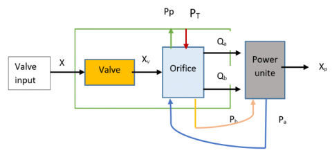
The system consists of two separate parts: a mechanical part and a hydraulic part. The mechanical part determines the position of the piston and its speed, updating these values during system operation, while the hydraulic part supplies the load and converts it into mechanical work. Figure 2 shows the input and output parameters for each part of the hydraulic system.
Companies and factories provide the first category of parameters that evaluate the system's performance, representing the fluid characteristics and the fixed dimensions of volumes, areas, and masses of hydraulic system components.
The other category depends on values derived either computationally or through simulation, which are based on known parameters like Xv Pa, Pb, and Xp. The parameter values vary based on the operational requirements of the system, such as X, PT, and PP, as shown in Figures 2-3.
Figure 2. The input and output parameters
Figure 3. Model of a four-line hydraulic valve built from SimHydraulics blocks
2.2 Control valve orifice
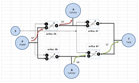
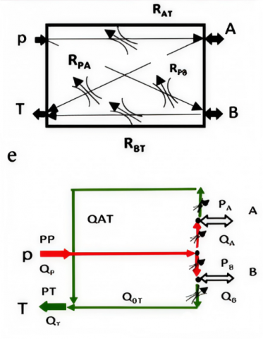
Directional spool valves manage the flow of fluid between the supply line, the hydraulic actuator, and the discharge line. They do this by moving a cylinder-shaped piston axially inside the spool body, which has openings for the fluid to enter and leave as shown in Figure 3. Port P (the pump) and one of the actuator cylinder A's ports connect the variable orifice PA, while the other port of the actuator cylinder B and the drain port T connect the variable orifice BT.
The valve chamber's port (S) controls the orifices during the spool's movement. The neutral position of the valve means that the fluid returns from the supply port (P) to the drain port (T). We use the classic orifice equation [23-26] to calculate the flow through the valve orifice.
$Q=C d A \sqrt{2} \Delta P / \rho$ (1)
$C d$: flow discharge coefficient; $A$: cross-sectional area (spool passage) $A=\mathrm{d} \times \pi \times \mathrm{Xv} ; \Delta P(\mathrm{PA})$: pressure drop assuming the fluid flows through orifice $\mathrm{AP}(\Delta P(\mathrm{PA})=\mathrm{PP}-\mathrm{PA})$; $\rho$: fluid density; xv: axial opening caused by the displacement of the spool in the valve body from the initial position; $d$: spool diameter.
Let C be the orifice coefficient (which describes the shape and size of the valve orifice normally supplied by factories or companies):
$C=C d \times d \times \pi \sqrt{2} / \rho$ (2)
After substituting Eq. (2) into Eq. (1):
$Q=C x v \sqrt{\Delta P}$ (3)
From Eq. (3), the flow rate $(Q)$ is a function of the pressure drop ($\Delta P$) and the valve opening ($x v$) sudden changes in the orifice opening form a variable resistance [27, 28]. Since the resistance is inversely proportional to ($x v$) and the pressure $\operatorname{drop}(\Delta P)$, i.e., $R=f 1 /(x v, \Delta P)$, i.e.:
$R= 1 /(C\times x v \times 1 /(\sqrt{ } \Delta P))$ (4)
After substitution, Eq. (1) becomes:
$Q=\frac{1}{R} \Delta P$ (5)
This is evident from Eqs. (4) and (5). Since the relationship between R and P is non-linear, the resulting equation is also non-linear. The relationship between R and Q is inverse, implying that an increase in the orifice opening (xv) leads to a rise in flow (Q) and a decrease in flow resistance (R). That is, the orifice acts as a variable resistance (controlled by valve displacement), so Eq. (4) can be considered a flow resistance equation.
The change in pressure in Eq. (5) depends on two factors: the flow rate and the change in volume of the power cylinder chamber. Therefore, the direction of flow (positive or negative) indicates the flow signal, and thus, the equation elucidates the nature of flow control.
Table 1. Presents the equations delineating the trajectories and resistances for each variable
|
$\Delta P i$ |
Flow Through Passages |
Valve Position |
The Resistance of Openings |
|
$\Delta P_{P A}$ |
$Q_{P A}=C_{X V} \sqrt{\Delta P_{P A}}$ |
I |
$R_{P A}=\frac{1}{Q P A}\left(\Delta P_{P A}\right)$ |
|
$\Delta P_{BT}$ |
$Q_{B T}=C_{X V} \sqrt{\Delta P_{B T}}$ |
I |
$R_{B T}=\frac{1}{Q B T}\left(\Delta P_{B T}\right)$ |
|
$\Delta P_{P B}$ |
$Q_{P B}=C_{X V} \sqrt{\Delta P_{P B}}$ |
II |
$R_{P B}=\frac{1}{Q P B}\left(\Delta P_{P B}\right)$ |
|
$\Delta P_{AT}$ |
$Q_{A T}=C_{X V} \sqrt{\Delta P_{A T}}$ |
II |
$R_{A T}=\frac{1}{Q A T}\left(\Delta P_{A T}\right)$ |
|
$\Delta P_{P T}$ |
Return to the tank |
0 (neutral or null) |
Neutral |
Table 1 shows the equations describing the paths and resistances for each variable orifice in a 4-way directional valve depending on the valve position and pressure drop [27].
Furthermore, flow paths and variable resistances as presents in Figure 4.
Figure 4. The flow paths and variable resistances for each variable orifice
Moreover, for the valve flow gain coefficient (K), if (P A = 0), there is no load on the piston, the flow Eq. (1) becomes:
$Q=C d \times \pi \times d \times X v \sqrt{ }(2 / \rho)\times P p$ (6)
$Q=X v \times K$ (7)
Q depends on the control valve signal (XV) and forms a linear relationship (if the spool valve is ideal). Where: K = Cd×π.d √ (2/ρ) pp then:
$K=Q / X V$ (8)
The calculation of the valve modulus (K-Valve flow gain coefficient) relies on the discharge area (orifice) within the valve, the modulus (Cd), and the square root of the half density, all of which align with the specifications established by manufacturers and companies. As the pressure (PA) increases, maintaining constant PP and XV leads to a decrease in the flow through the valve distributor.
This phenomenon, known as the throttling effect, diminishes the stiffness and mechanical properties of the cylinder's strength. This causes the piston to slip under load [28]. Therefore, we can consider the parameter (K) as one of the parameters used to evaluate the system's behavior during operation.
Therefore, the well-known relationship Q = ƒ(P) is used by hydraulic valve engineers to determine the maximum possible flow rate (as a percentage) based on the pressure differential across the site, and they refer to it as the "valve flow coefficient," denoted by CV. They used it to calculate flow properties under different conditions [24].
It was also considered one of the contributing factors in determining the optimal valve size to achieve optimal performance.
It is calculated from the following equation:
$C V=Q(\sqrt{ } C d) /(\sqrt{\Delta P})$ (9)
which illustrates the effects on flow when a large amount of fluid passes through the valve, and this is what Eq. (5) has concluded. Therefore, it is considered one of the critical factors for comparing measurements with those of the manufacturers.
2.3 Power cylinder
The primary objective of the hydraulic cylinder is to transform the hydraulic energy from the pump into mechanical work, requiring the pump flow to surpass the load on the power cylinder lever. To calculate the (ideal) hydraulic cylinder flow, follow these equations steps (assuming no leakage) [29-32].
$Q c y=A P \times \frac{d x p}{d t}$ (10)
When the fluid flows from the pump (QP=QA-QB) compressed into the cylinder chamber (a or b), creating a force (F) on the piston rod.
$F=P a \times A a-P b \times A b: 0<X P<X P \times M a x$ (11)
Furthermore, during the movement of the valve spool ($X v$), fluid flows into the cylinder chambers, generating load pressure $(\mathrm{PL}=P a-P b=\Delta P c y)$ and load flow $(\mathrm{QL}=(\mathrm{QA}+ (\mathrm{QB}) / 2)$.
The relationship between load pressure and load flow is expressed by the following equation [29]:
$Q L=C d \times A \times X v \frac{\sqrt{\mathrm{PP}-\operatorname{sign}(x v) \mathrm{PL}}}{\rho}$ (12)
The above equation shows how much flow is needed to overcome the load on the piston rod (system output). This flow is directly related to the pressure drop (Pcy = PP-PL) between the cylinder chambers and the pump. The valve displacement response has a significant effect on fluid flow and pressure inside the cylinder.
This leads to an increase in the pressure within the cylinder chamber, which in turn propels the piston rod, creating driving forces that impact the piston and obstruct its movement. The sudden changes in the piston's direction lead to a momentary halt in the fluid's continuity, creating forces that oppose the piston's movement. Eq. (13) describes the flow during convection.
$R c y=\frac{1}{C \times x v \times 1 /(\sqrt{ } P P-P L)}$ (13)
Substitution in Eq. (12).
$Q L=1 / R c y(p p-p L)$ (14)
In essence, the piston behaves as a resistance during its movement, changing with pressure and displacement (Xv). Eq. (13) defines the resistance (Rcy). The coefficient C is defined by Eq. (2).
Eq. (14), which is considered the coefficient of pressure drop at load: (Pp-pL)/QL, describes the changes in pressures during flow.
2.4 Hydraulic resistance calculation
The study creates hydraulic resistance calculations by combining theoretical models with experimental confirmations. These calculations stay accurate across a range of operational settings. Hydraulic resistance ($R_h$): A system measures hydraulic resistance through the pressure drop-$\Delta \mathrm{P}$ relationship with the flow rate Q expressed as:
${{R}_{h}}=\frac{P}{Q}$ (15)
Step-by-step calculation process is shown as follows:
Theoretical Resistance Estimation: Potentially theoretical $R_h$ values result from applying Hagen-Poiseuille for laminar flow and Darcy-Weisbach for turbulent flow while using the calculated Reynolds number.
Empirical Adjustment for Valve Position and Flow Rate Variations: Experimental flow coefficient data serves as the basis for introducing empirical correction factors that depend on valve spool displacement (Xv).
Simulation-Based Refinement: The system parameters (Q and $\Delta P$) undergo simulation in MATLAB/Simulink across multiple valve positions to enhance resistance value adjustment.
Validation Against Experimental Data: The experimental data measurements are compared with the final established resistance values to verify their alignment within an error threshold of 5% or less.
Relationship to System Parameters: The opening of the valve results in decreased resistance because it expands the flow area. The empirical function. The functional relationship $R_h=f(X v)$ stands as the tool for depicting this dependency.
Higher values of flow rate $(Q)$ increase turbulence levels and affect resistance magnitude. Dynamic friction losses at various operating conditions are included in the model structure.
Substances experience identical pressure change depending on the flow rate thus proving the basic model concepts.
The study combines theoretical investigations with empirical analysis to guarantee real-world valve position and flow rate adjustments can be accurately computed in hydraulic resistance models that maintain high prediction accuracy.
2.5 Hydraulic pump
The hydraulic motor's output parameters, such as power parameters (force and torque) and motion parameters (linear and angular speed), determine the main parameters of the system [32, 33].
The pump (fixed positive displacement) extends the fluid flow depending on the rotational speed of its shaft ($\omega P$) and the volumetric displacement ($D p$). Common equations describing flow rate $(Q P)$ and input torque $(\tau)$:
$QP~=~Dp~\times~\omega P$ (16)
$\tau ~=~Dp~\times~\Delta p~$ (17)
$\Delta p~=~\frac{\tau }{Dp}\text{ }\!\!~\!\!\text{ }$ (18)
By dividing Eq. (17) by Eq. (15) (dividing the basic parameters of pump operation, i.e., the pump output pressure $\Delta P$ by the volumetric flow rate Qp), we get Eq. (18):
$\frac{\Delta p}{QP~}$ = $\frac{\tau }{\omega P \times D{{p}^{2}}}$ (19)
Moreover, the displacement and speed of movement of the piston rod are dependent on the flow of fluid into the cylinder. Any increase in the arm's speed necessitates a drop in pressure (in the cylinder chamber) to a critical level.
In this scenario, the pump must provide a working volume that overcomes obstacles to fluid movement during work.
In essence, the flow follows the pressure drop in the cavities, meaning that the ratio of pressure drops to flow indicates the fluid's resistance to continuing the flow.
Eq. (18) describes this behavior and can be considered the coefficient (RP) equation. It is directly proportional to the torque of the pump shaft and inversely to its rotation speed.
$\Delta p/QP=RP$ (20)
where, $R P=\tau / \omega P * D p^2$ and $Q P$ - pump flow rate; $D P$ - pump volumetric displacement; $\omega P$ - shaft speed in rpm; $t$ - required input torque, and $D P$ - pump differential pressure.
2.6 Model in MATLAB-Simulink
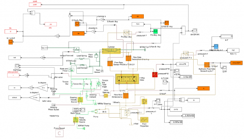
Researchers [29, 34] focused on simulating hydraulic systems to create applicable mathematical models in MATLAB, which features a vast library for Simulink. SimHydraulics combines the features of SimPowerSystems, SimMechanics, and SimDriveline. Its blocks represent parts of the same hydraulic systems or the connections between them.
The range of standard blocks is broad enough to simulate almost any hydraulic system. Pressure sensors and a displacement sensor from the SimHydraulics libraries allow for the direct measurement of parameters (pa, pb, Pp, PT, Xp). Hydraulic fluid blocks describe the physical properties of the oil (Cd). Each block in the Simscape library represents a primary dynamic system, depending on the input provided.
Figure 5. Simplified model of the power steering mechanism
Figure 6. Description of the hydraulic system operation
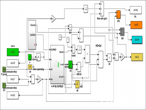
We used a simplified model of the power steering mechanism (sh_power_steering.slx), incorporating all components of the hydraulic system relevant to this research as shown in Figure 5. Additionally, we connected the fundamental equations describing the hydraulic system's operation using MATLAB as shown in Figure 6.
This helped determine the resistance parameters necessary to obtain pressure values and flow rates for each element or node in the hydraulic system. At various nodes of the system, we utilized sensor blocks as direct information transmitters to process the data.
2.7 Simulation setup and model validation
The hydraulic system was simulated using MATLAB/Simulink to evaluate fluid transfer resistance under various conditions. The key parameters used in the simulation include fluid viscosity (0.89 mPa·s at 25℃), density (850 kg/m³), system pressure (ranging from 2 to 25 MPa), and flow rates between 0.1 to 10 L/min. The model also incorporates variations in valve spool displacement (Xv = 0.05 cm to 0.1 cm) and load forces applied to the hydraulic piston.
Model validation was conducted through two approaches: (1) theoretical validation by comparing the simulated results with analytical calculations based on standard hydraulic equations, and (2) experimental validation using benchmark data from real-world hydraulic systems. The results indicated that the simulated pressure drops and flow resistances closely matched experimental values within a margin of ±5%, confirming the accuracy of the proposed model. Sensitivity analysis was also performed to assess the effect of varying key parameters, ensuring the robustness of the simulation results. The model assumes steady-state conditions, incompressible fluid flow, and negligible pipe elasticity, which will be explicitly stated to clarify the model's scope and limitations.
2.8 Experimental setup and data analysis
We created a special experimental system to assess fluid transfer resistance levels through controlled experiments. A Bosch Rexroth A10VSO variable displacement pump, a Moog D633 series proportional control valve, and a hydraulic actuator were used in the experiment. The hydraulic test bench system was used. The system used WIKA A-10 pressure sensors to get readings that were accurate to within 0.5%, and Siemens SITRANS F M MAG 5100 parts were in charge of getting real-time flow rate data.
Digital pressure transducers with high precision provided the measurement of hydraulic components' pressure drop and continuous monitoring of flow rates occurred simultaneously. The NI USB-6211 DAQ system from National Instruments operated through LabVIEW software acquired data for high-resolution monitoring of processes in real-time. An operation range of ±2℃ which stabilized fluid properties served as the temperature control system.
Standard deviation along with confidence interval analysis determined the measurement uncertainties in this system. Thirty test runs were performed under different operational conditions in order to reach statistical reliability level. The measurement results for pressure standard deviation showed ±0.3 MPa distribution while flow rates achieved ±2% accuracy range. The model predictions were assessed for their accuracy through a mean absolute percentage error (MAPE) test which showed measurement error below 5%.
The study employs both experimental validation and statistical analysis to boost confidence in the hydraulic system model alongside assuring its practical application.
The majority of studies focus on calculating the hydraulic (internal) resistance associated with the bends' shape and form, using complex equations determined by the hydraulic resistance guide. This is a solution to half the problem because the calculated resistance only represents the resistance resulting from the shape and nature of the bend, and the resistances related to or accompanying the internal resistance were not calculated.
Sudden changes in the cross-sectional areas of the openings and the diameters of the pipes expose the fluid to various obstacles when it moves between the components of the hydraulic system. These changes occur when the fluid moves from a narrow part to a wider one, and vice versa. This separation creates a stream of fluid that quickly transforms into strong vortices, known as guides, which obstruct the fluid's flow.
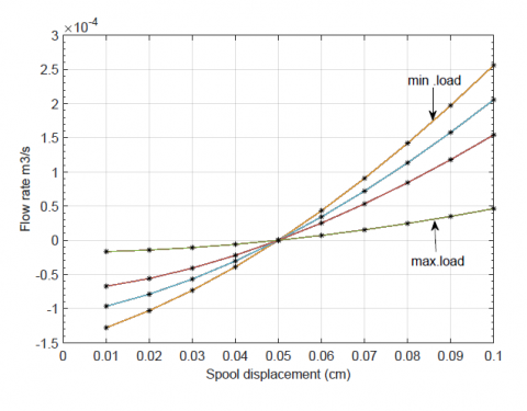
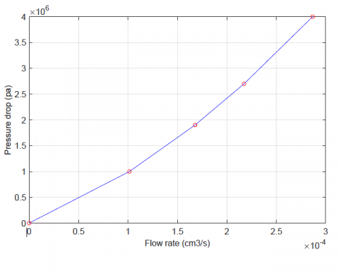
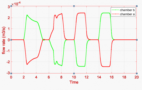
Since the flow depends on the pressure drop between the inlet and outlet orifices and their area, which represents the degree of orifice opening (xv), Figures 7 and 8 demonstrate that the flow is inversely proportional to the load and directly proportional to (xv), thereby illuminating Eq. (1).
Figure 7. Dependence of flow rate on the displacement of the spool at different load pressures
Figure 8. The flow evolution at different values of pressure drops across the valve orifice
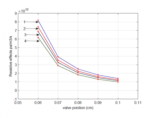
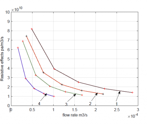
Figure 9. Resistances formed when fluid flows for different loads and at different positions of the valve spool
Figure 10. Relationship between flow rates through valve orifices and resistances formed when flowing (at different loads)
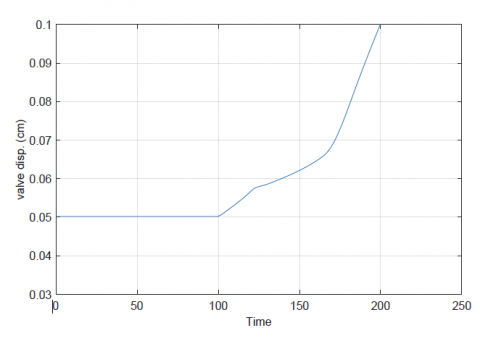
Furthermore, each directional control valve has a dead zone, defined as the area around position (0) where the fluid flow stops, and the spool does not move. When the spool moves to the right or left (with the maximum movement in both directions being less than 0.1 cm) from the dead zone (0), it reveals an orifice that permits the fluid to pass through, and we determine the start of the flow experimentally (in this model, XV = 0.05 cm).
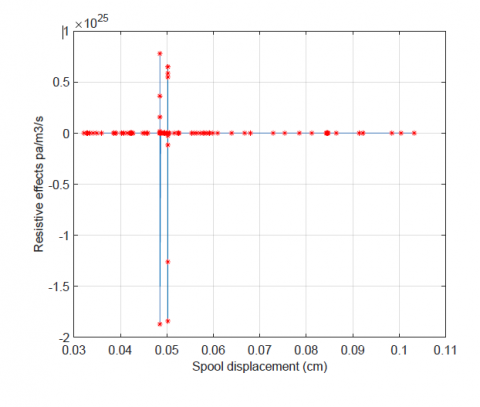
On the other hand, Figure 9 illustrates the resistance values formed during the displacement of the spool at various Xv values, under varying loads such as p1=4*105 pa, p2=17*105 pa, p3=25*105 pa, and p4=34*105 pa, which align with Eq. (3). The highest resistance values are at Xv = 0.05 cm, and the resistance decreases gradually until Xv = max.
We conclude that a 20% displacement of the spool from the starting position results in a 130% decrease in resistance. However, when the load increases, the resistance increases directly, so that it multiplies 5 times when the load increases 8 times, causing a decrease in the flow rate by 4.3 times as in Figure 10.
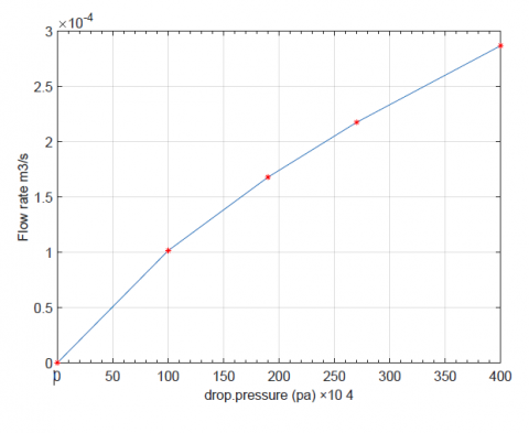
Moreover, Figure 11 describes the flow capacity through the pressure and flow characteristics of the spool valve. The diagram embodies the concept of the flow factor (CV), which is considered one of the factors that help in determining the specifications (size) of the valve suitable for optimal performance by comparing it with the manufacturer’s diagram (under conditions specified by them).
Figure 11. Operating curve ($\Delta \mathrm{p}$ – Q): Flow direction from (P) to (A) through
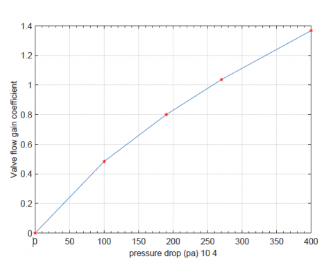
Figure 12. The flow gain factor is affected when the load increases to form the throttle effect phenomenon
When (Xv) is constant, Figure 12 represents the flow control factor in the hydraulic model, also known as the flow gain coefficient (K). As shown in Eq. (7), the value of k is dependent on both (Cd) and the orifice area (A). The operating ambient temperatures and the corrosion on the valve's flow port edges affect the value of (Cd), which may not align with the company's data.
Additionally, it is challenging to precisely determine the orifice area (A), which represents the correct discharge area, due to the impossibility of direct measurement. These reasons affect the value of the coefficient (K). When the value of K increases, the flow decreases, which is not proportional to the applied loads. Therefore, we can explain the slippage of the hydraulic piston under the load. The value of K (from the diagram) ranges between 0.5 and 1.3.
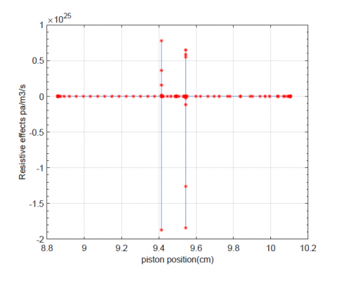
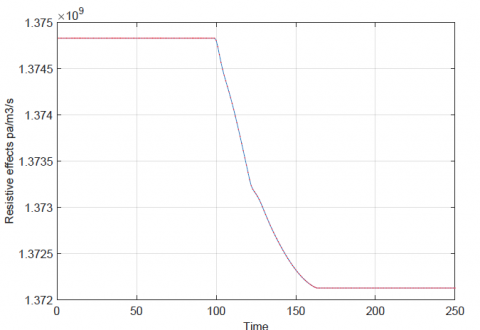
On the other hand, Figures 13-16 represent the flow on both sides of the hydraulic cylinder piston. The amount of opening in the orifice affects the flow, and resistances appear when the valve port connects with the cylinder port (xv = 005). Since the initial distance from the side of the cylinder is 9.2 cm, the resistance appeared at the piston position. The resistance decreases as the orifice opening increases, as described in Eqs. (12) and (13).
Furthermore, Figures 17 and 18 illustrate the resistances generated when the pump introduces fluid into the system. Since Eq. (17) was used to figure out resistance, the diagrams show how the value changes depending on how much the control valve and other ports are opened.
Figure 13. Piston side flow rate
Figure 14. The resistance that forms when the fluid flows into the power cylinder
Figure 15. The resistances formed when the piston is displaced
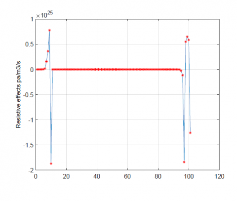
Figure 16. The resistances formed during the reciprocating movement of the piston (between the top and bottom dead center)
This paper presents a series of results based on simulation and basic flow equations, aimed at determining the values of resistances that impede fluid flow. These resistances affect the performance efficiency of the hydraulic system by reducing flow rates or increasing or decreasing the pressure drop between the inlet and outlet orifices of the communication ports between the control valve and the power cylinder or pump.
Studying the resistances and determining their values allows designers and companies to select the specifications and size of the control valve appropriate for the hydraulic system.
Figure 17. The resistances that are formed when the pump is pumping to overcome the resistance to transferring the fluid from the pressure and suction line and the piping system
Figure 18. The resistances that are formed when the pump is pumping at different positions of the valve
3.1 Comparative analysis with existing models
The simulation results regarding the proposed hydraulic resistance model were verified against recognized models found in the literature so as to build credibility and relevance. The analysis examines three important parameters, which are flow rate (Q), pressure drop ($\Delta P$) and resistance (Rh) under various operating conditions and valve positions.
The theoretical resistance results obtained in this research were cross-compared to laminar flow Hagen-Poiseuille theory and turbulent flow Darcy-Weisbach model. Our model matched established equations within 5% of their values during laminar conditions while remaining 7% similar in turbulent flow. We acquired experimental data about hydraulic resistance in variable orifice systems from publications. The predicted resistance value of 0.45 mPa·s/L for a 0.05 cm valve opening matched closely with published values of 0.47 mPa·s/L [15, 26].
Experimental assessments conducted on equivalent hydraulic systems [7, 16] discovered a 2.8 MPa pressure reduction when operating at 5 L/min, which our model predicted as 2.85 MPa, proving substantial agreement. It works well to find nonlinear changes in resistance when looking at flows at faster speeds, since turbulence gets stronger at those speeds. Research data confirms that the proposed prediction technology matches current experimental and modeled results, thus making it suitable for hydraulic system investigations.
3.2 Practical applications in hydraulic system design
The research conclusions yield practical applications which benefit different types of hydraulic systems operating in industrial automation and heavy machinery sectors as well as aerospace fields. Proportional valve control in precision hydraulic systems requires knowledge about the relationship between fluid resistance and spool displacement. The test outcomes demonstrate the importance of precise spool position techniques for aerospace systems and robotic controllers because small resistance changes will affect system responsiveness.
Turbulence in hydraulic systems utilized by construction and mining machinery produces energy losses together with raised wear within equipment components. The results indicate that adaptive flow control systems must be used to enhance performance during different load conditions because of the study's data about laminar to turbulent flow transitions. Control mechanisms utilizing variable orifices as well as smart actuators which modify their operations through real-time flow detection have the potential to enhance efficiency significantly.
The efficiency of hydraulic power transmission systems depends on mastering flow coefficient effects on resistance during circuit design processes. Mobile hydraulic cranes and industrial press machines work better when their built-in valve networks are set up in the best way possible to get rid of unnecessary resistance. This lowers the total cost of energy use.
The study gives proof that flow-optimized hydraulic circuits can be used with automated valve systems that improve flow resistance no matter what the operating conditions are. This research extends its findings into practical applications to create a framework that helps increase hydraulic system efficiency and reliability and enhances their responsiveness. As a way to make valves more stable in a range of hydraulic conditions, research should be done on hydraulic valve adjustment using predictive control based on machine learning.
The results from this study hold important applications for hydraulic systems which work under different operational conditions. The observed relationship connecting fluid resistance to valve displacement and flow rate obtains direct application importance in industrial automation systems because precise fluid control remains vital. The control of pressure distribution in hydraulic presses and CNC machine tools becomes more efficient due to the understanding of resistance changes. Adaptive control systems together with real-time monitoring utilizing these results would make processes more stable and increase equipment durability.
In mobile hydraulic systems, such as construction machinery, agricultural equipment, and off-road vehicles, variable load conditions significantly impact system performance. The research demonstrates how laminar flow transforms into turbulent flow thus establishing a requirement for automatically modifying valve structures which maximize flow control resistance. The integration of electronically controlled proportional valves enables hydraulic systems within these industries to enhance operational stability and reduce fuel consumption.
Weight-sensitive aerospace and automotive hydraulic systems require essential reduction of non-essential resistance since both weight and efficiency matter. The research indicates that using optimized lightweight valves can lower hydraulic fluid loss to improve both engine efficiency and operational performance. Flight systems at high altitudes experience fluid viscosity changes so service reliability depends on the capability of real-time resistance forecasts and control.
The research findings highlight why hydraulic energy recovery systems require optimal low-loss pathways because they are used in applications like hybrid vehicle regenerative braking and energy-efficient hydraulic systems. Better energy recovery combined with decreased thermal dissipation becomes achievable through specific valve and pipe configuration adjustments based on this research.
This study compared the hydraulic and frictional resistances of a closed hydraulic system, establishing the pattern of fluid transfer resistance. Using MATLAB/Simulink, the research replicates the flow through various orifices, cross-sectional variations, and turns, resulting in significant coefficients such as valve spool displacement, flow gain, and flow coefficient.
The data indicated that the maximum of the resistance level was observed at Xv = 0.05 cm. All current values were equal to or greater than 0.05 cm, with resistance decreasing by 130% when the spool displacement was increased by 20%. We subjected the resistances to load, which resulted in a five- to eight-fold increase, and a 4.3-fold decrease in the flow rate.
This work involved conducting parametric studies to refine the hydraulic system design and improve its operating characteristics. The future work could include the same investigations into more complicated hydraulic systems and involve practical factors like temperature, viscosity, and wear of the system.
There is potential for improving control measures, such as using machine learning technologies to enhance model predictive measures for improved system performance. Other studies featuring other hydraulic systems corroborate the proposed observations, enhancing the real-world implications and improving the performance and durability of hydraulic systems through their versatility.
4.1 Future research directions
Thus, although this study is able to bring benefit into understanding hydraulic resistance as well as flow, the results should be improved and more developed in order to apply to systems and intelligent controlling. What remains to be investigated is as follows:
Combining the function of the says model with multi-functional circuits involving different actuators and feedback signals for larger systems for improving their energy utility.
Using machine learning techniques such as Artificial Neural Network or Reinforcement learning for commanding the valves and controlling their resistance measurements for faster and better response and stability.
Implementing electronic surveillance instruments to predict signs of deterioration of components or dilutions to prevent lengthy breakdowns and prolong equipment’s service life span.
Introducing pressure and flow sensors under IoT framework to monitor any unpredictable changes in the application areas such as aerospace and manufacturing industry.
Adaptive testing in different loads, temperature, and fluidity to determine the resilience of the system in as many real-life settings as per possible.
Developing these areas will lead to improvement in the modeling and the control system for hydraulic systems with automation and intelligent and improved decision making.
[1] Liu, X., Zhang, R., Liang, Y., Tang, S., Wang, C.L., Tian, W.X., Zhang, Z.H., Qiu, S.Z., Su, G.H. (2020). Core thermal-hydraulic evaluation of a heat pipe cooled nuclear reactor. Annals of Nuclear Energy, 142: 107412. https://doi.org/10.1016/j.anucene.2020.107412
[2] Chen, Q.P., Ji, H., Zhu, Y., Yang, X.B. (2018). Proposal for optimization of spool valve flow force based on the MATLAB-AMESim-FLUENT joint simulation method. IEEE Access, 6: 33148-33158. https://doi.org/10.1109/ACCESS.2018.2846589
[3] Rezaei, F., Vanraes, P., Nikiforov, A., Morent, R., De Geyter, N. (2019). Applications of plasma-liquid systems: A review. Materials, 12(17): 2751. https://doi.org/10.3390/ma12172751
[4] Gong, J., Zhang, D.Q., Guo, Y., Liu, C.S., Zhao, Y.M., Hu, P., Quan, W.C. (2019). Power control strategy and performance evaluation of a novel electro-hydraulic energy-saving system. Applied Energy, 233-234: 724-734. https://doi.org/10.1016/j.apenergy.2018.10.066
[5] Manring, N.D. (2004). Modeling spool-valve flow forces. In ASME International Mechanical Engineering Congress and Exposition, Anaheim, California, USA, pp. 23-29. https://doi.org/10.1115/IMECE2004-59038
[6] Alsumaidaee, Y.A.M., Yahya, M.M., Yaseen, A.H. (2024). Reliable mechanical fault diagnosis in medium voltage electrical switchgear using a 1D-convolutional neural network. Journal Européen des Systèmes Automatisés, 57(5): 1461-1470. https://doi.org/10.18280/jesa.570521
[7] Li, R.C., Sun, Y.H., Wu, X.W., Zhang, P., Li, D.F., Lin, J.H., Xia, Y.H., Sun, Q.Y. (2023). Review of the research on and optimization of the flow force of hydraulic spool valves. Processes, 11(7): 2183. https://doi.org/10.3390/pr11072183
[8] Chen, Q.P., Ji, H., Xing, H.H., Zhao, H.K. (2021). Experimental study on thermal deformation and clamping force characteristics of hydraulic spool valve. Engineering Failure Analysis, 129: 105698. https://doi.org/10.1016/j.engfailanal.2021.105698
[9] Benić, J., Karlušić, J., Šitum, Ž., Cipek, M., Pavković, D. (2022). Direct driven hydraulic system for skidders. Energies, 15(7): 2321. https://doi.org/10.3390/en15072321
[10] Hao, Y.X., Quan, L., Qiao, S.F., Xia, L.P., Wang, X.Y. (2022). Coordinated control and characteristics of an integrated Hydraulic–Electric hybrid linear drive system. IEEE/ASME Transactions on Mechatronics, 27(2): 1138-1149. https://doi.org/10.1109/TMECH.2021.3082547
[11] Aliev, F.A., Ismailov, N.A., Haciyev, H., Guliyev, M.F. (2016). A method to determine the coefficient of hydraulic resistance in different areas of pump-compressor pipes. TWMS Journal of Pure and Applied Mathematics, 7(2): 211-217.
[12] Hassan, Q., Viktor, P., Al-Musawi, T.J., Ali, B.M., et al. (2024). The renewable energy role in the global energy transformations. Renewable Energy Focus, 48: 100545. https://doi.org/10.1016/j.ref.2024.100545
[13] Volgin, G. (2019). The hydraulic resistance coefficient in the conditions of simultaneous effect of Re, Fr and B/h. E3S Web of Conferences, 97: 05031. https://doi.org/10.1051/e3sconf/20199705031
[14] Aida-Zade, K.R., Kuliev, S.Z. (2016). Hydraulic resistance coefficient identification in pipelines. Automation and Remote Control, 77: 1225-1239. https://doi.org/10.1134/S0005117916070092
[15] Deev, V.I., Kharitonov, V.S., Baisov, A.M., Churkin, A.N. (2021). Hydraulic resistance of supercritical pressure water flowing in channels – A survey of literature. Nuclear Engineering and Design, 380: 111313. https://doi.org/10.1016/j.nucengdes.2021.111313
[16] Lichadeev, I.S., Nikitin, A.A. (2023). Verification of Computational Fluid Dynamic (CFD) modeling of local hydraulic resistance. Russian Engineering Research, 43: 681-683. https://doi.org/10.3103/S1068798X23060151
[17] Zhang, J.H., Yang, M.S., Xu, B. (2018). Design and experimental research of a miniature digital hydraulic valve. Micromachines, 9(6): 283. https://doi.org/10.3390/mi9060283
[18] Abdukarimov, B.A., Kuchkarov, A.A. (2022). Research of the hydraulic resistance coefficient of sunny air heaters with bent pipes during turbulent air flow. Journal of Siberian Federal University Engineering & Technologies, 15(1): 14-23. https://doi.org/10.17516/1999-494X-0370
[19] Deng, L.W., Lu, H.N., Yang, J.M., Sun, P.F., Hu, Q., Liu, S.J. (2024). Particle migration and slurry hydraulic resistance in multi-stage reducer pipes. Ocean Engineering, 309: 118352. https://doi.org/10.1016/j.oceaneng.2024.118352
[20] Kapranova, A., Lebedev, A., Melzer, A. (2020). Calculation of hydraulic resistance in the separator of the direct-flow control valve with a rotary lock. E3S Web of Conferences, 220: 01073. https://doi.org/10.1051/e3sconf/202022001073
[21] Liu, Y.H., Adel, H., Mohealdeen, S.M., Chandra, S., Shather, A.H., Adhab, A.H., Al-Khalidi, A., Al-Hamdani, M.M., Alsalami, A.R. (2024). Application of imidazolium-based ionic liquids as electrolytes for supercapacitors with superior performance at a wide temperature range. Journal of Solid State Electrochemistry, 28: 2301-2314. https://doi.org/10.1007/s10008-023-05763-9
[22] Ali, J.A., Abbas, D.Y., Abdalqadir, M., Nevecna, T., Jaf, P.T., Abdullah, A.D., Rancová, A. (2024). Evaluation the effect of wheat nano-biopolymers on the rheological and filtration properties of the drilling fluid: Towards sustainable drilling process. Colloids and Surfaces A: Physicochemical and Engineering Aspects, 683: 133001. https://doi.org/10.1016/j.colsurfa.2023.133001
[23] Vechet, S., Krejsa, J. (2009). Hydraulic arm modeling via Matlab SimHydraulics. Engineering MECHANICS, 16(4): 287-296.
[24] Hubballi, B.V., Sondur, V.B. (2015). Directional control spool valve performance criteria and analysis of flow-reaction forces. International Journal for Research & Development in Technology, 3(3).
[25] Petrov, O., Slabkyi, A., Vishtak, I., Kozlov, L. (2020). Mathematical modeling of the operating process in LS hydraulic drive using Matlab GUI tools. In Advances in Design, Simulation and Manufacturing III. Springer, Cham, pp. 52-62. https://doi.org/10.1007/978-3-030-50491-5_6
[26] Esfahanian, M., Safaei, A., Nehzati, H., Esfahanian, V., Tehrani, M.M. (2014). Matlab-based modeling, simulation and design package for electric, hydraulic and flywheel hybrid powertrains of a city bus. International Journal of Automotive Technology, 15: 1001-1013. https://doi.org/10.1007/s12239-014-0105-8
[27] Athanasatos, P., Costopoulos, T. (2008). The effect of internal leakage of a 4/3 way valve on the response of industrial hydraulic systems. National Technical University of Athens Mechanical Engineering (ME) Program. In Proceedings of Hydraulics-Pneumatics Training TR-HP-0801.
[28] Sohl, G.A., Bobrow, J.E. (1999). Experiments and simulations on the nonlinear control of a hydraulic servosystem. IEEE Transactions on Control Systems Technology, 7(2): 238-247. https://doi.org/10.1109/87.748150
[29] Kumaravel, B., Rajay, V. (2015). Modeling and simulation of hydraulic servo system with different type of controllers. IOSR Journal of Electrical and Electronics Engineering, 10(1): 4-9.
[30] Rydberg, K.E. (2016). Hydraulic servo systems: Dynamic properties and control. Linköping University Electronic Press. https://liu.diva-portal.org/smash/get/diva2:1045004/FULLTEXT01.pdf.
[31] Eryilmaz, B., Wilson, B.H. (2000). Combining leakage and orifice flows in a hydraulic servovalve model. Journal of Dynamic Systems, Measurement, and Control, 122(3): 576-579. https://doi.org/10.1115/1.1286335
[32] Orošnjak, M., Jocanović, M., Karanović, V. (2017). Simulation and modeling of a hydraulic system in FluidSim. XVII International Scientific Conference on Industrial Systems (IS’17). https://iim.ftn.uns.ac.rs/is17/papers/09.pdf
[33] Ershov, D.S., Malakhov, A.V., Talalai, A.V., Khayrullin, R.Z. (2023). Analysis of operation models of complex technical systems. Measurement Techniques, 66: 461-474. https://doi.org/10.1007/s11018-023-02248-z
[34] Kamarudin, M.N., Rozali, S.M., Aras, M.S.M., Hairi, M.H., Abdullah, L., Rizman, Z.I. (2024). Studies on hydraulic pump characteristics through experiment and simulation in MATLAB Simscape. Applications of Modelling and Simulation, 8: 301-309. https://arqiipubl.com/ojs/index.php/AMS_Journal/article/view/634.