Khaled Habri*![]() | Zin-Eddine Azzouz
| Zin-Eddine Azzouz![]() | Karim Negadi
| Karim Negadi![]() | Abdenbi Mimouni
| Abdenbi Mimouni![]()
© 2025 The authors. This article is published by IIETA and is licensed under the CC BY 4.0 license (http://creativecommons.org/licenses/by/4.0/).
OPEN ACCESS
This paper introduces a hybrid computational method for characterizing far-field electromagnetic radiation from lightning over a perfectly conducting ground. The method combines the Finite-Difference Time-Domain (FDTD) technique with Sommerfeld integrals to address the high memory demands associated with large simulation domains. It enables efficient field mapping by reducing memory usage by up to 90% compared to full-domain FDTD, while maintaining high accuracy. The approach is computationally scalable, making it well-suited for analyzing complex geometries and large-scale scenarios relevant to lightning modeling and electromagnetic compatibility (EMC) studies. By significantly lowering the computational burden, the method allows for simulations that would be impractical using conventional techniques. Future developments will aim to further accelerate the computation, incorporate realistic ground conditions, and extend the model to three-dimensional configurations for broader applicability.
absorbing boundary conditions, FDTD method, electromagnetic compatibility, lightning electromagnetic field, Maxwell's equations, Sommerfeld integrals
Several studies focusing on the characterization of lightning-induced electromagnetic radiation have primarily aimed at developing computational methods to model this phenomenon as accurately as possible. The main objective is to establish reliable predictive models that can be implemented numerically to simulate lightning’s electromagnetic radiation, thereby reducing the costs associated with experimentation. Two main approaches are commonly distinguished in this field: analytical methods, which reduce the problem of electromagnetic radiation to the evaluation of specific integrals known as "Sommerfeld integrals"—which can be challenging in terms of convergence without simplifying assumptions (such as the assumption of a perfectly conducting ground)—and numerical methods, which solve Maxwell’s equations using a predefined spatial mesh.
One of the major challenges in numerical methods lies in the infinite extent of the analysis domain, necessitating artificial truncation through the introduction of appropriate boundary conditions. These conditions, referred to as "Absorbing Boundary Conditions" (ABC), aim to minimize non-physical reflections at the boundaries, making them nearly transparent to waves propagating outward. These conditions are also referred to as transparent, non-reflective, radiation, free-space, or open conditions when they are written in asymptotic form.
The assumption of a perfectly conducting ground has significantly simplified the electromagnetic field equations over distances of a few kilometers, as demonstrated by several researchers [1-3]. Two main approaches are used to obtain the electromagnetic field waveforms in the time domain: the first is based on Maxwell’s equations and the image theory [4], while the second involves making the soil conductivity tend toward infinity in Sommerfeld integrals [5].
In this study, we focus on characterizing the electromagnetic radiation of lightning under the assumption of a perfectly conducting ground. To achieve this, we have developed computational codes within the MATLAB environment, utilizing a numerical approach based on the Finite-Difference Time-Domain (FDTD) method. The main contribution of our work lies in the proposal of a new type of absorbing boundary conditions. Unlike conventional conditions, these are determined analytically by numerically evaluating Sommerfeld integrals at the fictitious boundaries of the domain, independently of the internal field values. This hybrid approach thus combines an analytical method (Sommerfeld integrals) with a numerical method FDTD to enhance the modeling of lightning-induced electromagnetic fields.
While several studies have explored hybrid approaches combining FDTD and Sommerfeld integrals for lightning field simulations, our work introduces an innovative way of integrating analytically computed absorbing boundary conditions. Unlike conventional techniques such as Mur’s ABC or Perfectly Matched Layer (PML) [6-15], our approach enhances the accuracy of wave propagation by rigorously defining boundary values.
This methodology is particularly advantageous for long-distance simulations, where conventional numerical ABCs introduce errors. Furthermore, we demonstrate significant memory savings without compromising accuracy, making this method suitable for large-scale computations.
It is worth noting that most previous studies combining the FDTD method with Sommerfeld integrals have primarily focused on improving far-field calculations or modeling multilayered ground structures [6, 7]. However, they have not directly addressed how to leverage the analytical structure of Sommerfeld integrals to generate boundary conditions specifically tailored for FDTD models in the time domain. These studies often relied on approximate solutions or frequency-domain transformations without explicit analytical incorporation in the time domain [8]. This reveals a research gap that the present work aims to fill: the lack of a hybrid methodology that connects accurate analytical calculations at the external boundaries using Sommerfeld integrals with numerical computation within the domain using FDTD, in a way that ensures high accuracy and physically consistent wave propagation.
The innovative aspect of this work lies in developing a new type of absorbing boundary condition, calculated numerically through Sommerfeld integrals at the domain boundaries. This eliminates the dependence on traditional boundary conditions such as Mur or PML and significantly reduces nonphysical reflections. Unlike previous approaches that implement these two methods separately or approximately, our approach integrates them explicitly within the numerical solving loop.
The potential contributions of this work include, from a theoretical perspective, introducing a new framework for modeling electromagnetic wave propagation in FDTD environments with analytically defined open boundaries. On the practical side, the approach enhances simulation performance for lightning-induced electromagnetic fields over long distances without the need for excessively large computational domains or high memory usage. Moreover, the methodology enables the development of more accurate models for electromagnetic protection system design or lightning interference level assessment.
This is how the rest of the paper is organized: In Section 2, the electromagnetic field is mathematically modeled, focusing on Maxwell’s equations and their adaptation to cylindrical coordinates. Section 3 outlines the fundamental principles of the FDTD method, including spatial and temporal discretization techniques. Section 4 introduces a novel approach to absorbing boundary conditions based on Sommerfeld integrals, improving the efficiency and accuracy of numerical simulations. Section 5 discusses the implementation of boundary conditions at the ground plane, assuming a perfectly conducting ground to simplify the equations. Section 6 presents simulation results and a comparative analysis with conventional techniques, highlighting memory efficiency improvements. Finally, Section 7 concludes the paper by summarizing key findings and proposing potential future research directions.
Equations of Maxwell’s describe all electromagnetic phenomena. The FDTD method [9-13] facilitates their resolution within the computational domain by incorporating boundary conditions and reformulating them into a system of algebraic equations. Solving this system enables the determination of the spatiotemporal electromagnetic field distribution at a given mesh's nodes.
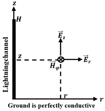
Figure 1. Problematic geometry of electromagnetic radiation from lightning [9]
For clarity, a consistent notation is adopted for Maxwell’s equations and their transformation into cylindrical coordinates (see Figure 1). These field equations are formulated as follows [9, 14, 15]:
$\vec{\nabla} \times \vec{E}=-\mu . \frac{\partial \vec{H}}{\partial t}$ (1)
$\vec{\nabla} \times \vec{H}=\sigma . \vec{E}+\varepsilon . \frac{\partial \vec{E}}{\partial t}$ (2)
where:
$\vec{E}:$ is the electric field,
$\vec{H}:$ denotes the magnetic field,
$\mu:$ represents the magnetic permeability,
$\varepsilon:$ corresponds to the dielectric permittivity,
$\sigma:$ denotes the electrical conductivity.
The following form can be used to express the partial differential equations that come from mathematically developing Eqs. (1) and (2) using a spatial representation in a cylindrical coordinate system:
$\left\{\begin{array}{c}\frac{\partial H_{\varphi}}{\partial t}=\frac{1}{\mu}\left[\frac{\partial E_z}{\partial r}-\frac{\partial E_r}{\partial z}\right] \\ \sigma E_r+\varepsilon \frac{\partial E_r}{\partial t}=\frac{\partial H_{\varphi}}{\partial z} \\ \sigma E_z+\varepsilon \frac{\partial E_z}{\partial t}=\frac{1}{r} \frac{\partial}{\partial r}\left(r H_{\varphi}\right)\end{array}\right.$ (3)
where:
$E_r:$ is the horizontal electric field,
$E_z:$ is the vertical electric field,
$H_{\varphi}:$ is the azimuthal magnetic field,
$z:$ is the elevation of the observation site relative to the ground,
$r:$ is the horizontal separation between the lightning channel and the observation location.
The previous expression can be made as follows in the computation region (above ground) where $\sigma=0$, $\varepsilon=\varepsilon_0$, and $\mu=\mu_0$ are present:
$\left\{\begin{array}{c}\frac{\partial H_{\varphi}}{\partial t}=\frac{1}{\mu_0}\left[\frac{\partial E_z}{\partial r}-\frac{\partial E_r}{\partial z}\right] \\ \varepsilon_0 \frac{\partial E_r}{\partial t}=\frac{\partial H_{\varphi}}{\partial z} \\ \varepsilon_0 \frac{\partial E_z}{\partial t}=\frac{1}{r} \frac{\partial}{\partial r}\left(r H_{\varphi}\right)\end{array}\right.$ (4)
3.1 Discretization in space and time
The FDTD technique is used to solve the system of partial differential Eq. (4) [9]. First, we assume a spatiotemporal scalar function f(r,z,t) defined at every point p(r,z) belonging to a finite space $\Omega$ and every time t belongs to a finite interval of time $\psi$ in order to illustrate the fundamental idea of this resolution:
$[p(r, z) \in \Omega] \Leftrightarrow\left\{\begin{array}{l}r_{\min } \leq r \leq r_{\max } \\ z_{\min } \leq z \leq z_{\max }\end{array}\right.$ (5)
$t \in \psi \Leftrightarrow t_{min } \leq t \leq t_{max }$ (6)
The spatial discretization (mesh) in r and z directions with space steps $\Delta r$ and $\Delta z$, respectively, creates a network of nodes whose positions are determined by:
$\left\{\begin{array}{l}r=r_i=r_{min }+i . \Delta r \\ z=z_j=z_{min }+j . \Delta z\end{array}\right.$ (7)
The following formula represents the temporal discretization with a step $\Delta t:$
$t=t_n=t_{min }+n . \Delta t$ (8)
where, n: an increase in time.
As a result, the function f can be evaluated as follows at any node and at any time:
$f(r, z, t)=f\left(r_{min }+i \Delta r, z_{min }+j \Delta z, t_{min }+n \Delta t\right)=f^n(i, j)$ (9)
with: $\left\{\begin{array}{c}0 \leq i \leq i_{max } \\ 0 \leq j \leq j_{max } \\ 0 \leq n \leq n_{max }\end{array}\right.$.
The partial derivatives of function f are approximated at the first order level as follows [9]:
$\left\{\begin{array}{l}\left.\frac{\partial f(r, z, t)}{\partial r}\right|_{i \Delta r}=\frac{f^n\left(i+\frac{1}{2}, j\right)-f^n\left(i-\frac{1}{2}, j\right)}{\Delta r} \\ \left.\frac{\partial f(r, z, t)}{\partial z}\right|_{j \Delta z}=\frac{f^n\left(i, j+\frac{1}{2}\right)-f^n\left(i, j-\frac{1}{2}\right)}{\Delta z} \\ \left.\frac{\partial f(r, z, t)}{\partial t}\right|_{n \Delta t}=\frac{f^{n+\frac{1}{2}}(i, j)-f^{n-\frac{1}{2}}(i, j)}{\Delta t}\end{array}\right.$ (10)
3.2 Dissecting the equations for the electromagnetic field
The elements of the electromagnetic field emitted by lightning can be written as follows using the system's partial differential Eq. (4) and the basic idea of the FDTD approach described in Eq. (10).
$E_z^{n+1}\left(i, j+\frac{1}{2}\right)=E_z^n\left(i, j+\frac{1}{2}\right)+\frac{\Delta t}{\varepsilon_0 . r_i . \Delta r}\left[\left(r_{i+\frac{1}{2}}\right) . H_{\varphi}^{n+\frac{1}{2}}\left(i+\frac{1}{2}, j+\frac{1}{2}\right)-\left(r_{i-\frac{1}{2}}\right) . H_{\varphi}^{n+\frac{1}{2}}\left(i-\frac{1}{2}, j+\frac{1}{2}\right)\right]$ (11)
with: $\left\{\begin{array}{c}0 \leq i \leq i_{max } \\ 0 \leq j \leq j_{max }-1 \\ 0 \leq n \leq n_{max }-1\end{array}\right.$.
$E_r^{n+1}\left(i+\frac{1}{2}, j\right)=E_r^n\left(i+\frac{1}{2}, j\right)-\frac{\Delta t}{\varepsilon_0 . \Delta z}\left[H_{\varphi}^{n+\frac{1}{2}}\left(i+\frac{1}{2}, j+\frac{1}{2}\right)-H_{\varphi}^{n+\frac{1}{2}}\left(i+\frac{1}{2}, j-\frac{1}{2}\right)\right]$ (12)
with: $\left\{\begin{array}{c}0 \leq i \leq i_{max }-1 \\ 1 \leq j \leq j_{max } \\ 0 \leq n \leq n_{max }-1\end{array}\right.$.
$H_{\varphi}^{n+\frac{1}{2}}\left(i+\frac{1}{2}, j+\frac{1}{2}\right)=H_{\varphi}^{n-\frac{1}{2}}\left(i+\frac{1}{2}, j+\frac{1}{2}\right)+\frac{\Delta t}{\mu_0 . \Delta r} .\left[E_z^n\left(i+1, j+\frac{1}{2}\right)-E_z^n\left(i, j+\frac{1}{2}\right)\right]-\frac{\Delta t}{\mu_0. \Delta z} .\left[E_r^n\left(i+\frac{1}{2}, j+1\right)-E_r^n\left(i+\frac{1}{2}, j\right)\right]$ (13)
with: $\left\{\begin{array}{c}0 \leq i \leq i_{max }-1 \\ 0 \leq j \leq j_{max }-1 \\ 0 \leq n \leq n_{max }-1\end{array}\right.$.
Lastly, it should be mentioned that the time step $\Delta t$ and the spatial steps $\Delta r$ and $\Delta z$ must satisfy a stability calculation requirement, which is represented by the following equation:
$\Delta t<\frac{min (\Delta r, \Delta z)}{2 c}$ (14)
where, c represent the light velocity.
You can also refer to the references [9, 16-25] for additional information on the FDTD approach.
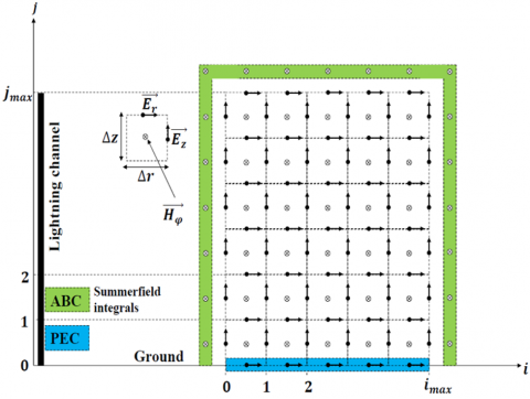
Restricting the computing domain is required when employing finite difference methods to solve time-domain electromagnetic field equations in an unbounded space. In order to simulate the unbounded environment, the mesh is truncated and ABC are applied at its artificial bounds (see Figure 2).
Numerous absorbing border conditions are presented in the literature with the goal of minimizing reflections at the boundaries of the computational domain. The PML [26], the Complementary Boundary Operator (CBO) [27], the Low Frequency Boundary Algorithm (LFBA) [28], and Mur's boundary conditions [29] are some of the most often utilized.
Figure 2. FDTD in cylindrical coordinates for 2D mesh
We suggest a different kind of absorption barrier in this study, in which the magnetic field values at the boundaries are assessed analytically separately from the field values inside the analysis zone.
Assuming a perfectly conducting ground, the boundary calculations will primarily focus on determining the Sommerfeld integrals [9] that describe the magnetic field (Figure 2).
One advantage of this boundary type is that it allows the lightning channel to be excluded from the analysis region, as the internal electromagnetic field values will be adjusted based on the pre-calculated values at the boundaries. This property is crucial for reducing the size of the matrices involved in the calculation. The following expressions illustrate how these boundaries are computed:
4.1 In the horizontal direction
$H_{\varphi}^{n+\frac{1}{2}}\left(-\frac{1}{2}, j+\frac{1}{2}\right)=\frac{r_{-\frac{1}{2}}}{4 \pi} \int_{-H}^H\left[\frac{i\left(z^{\prime}, t_{n+\frac{1}{2}}-\frac{R_{-\frac{1}{2}, j+\frac{1}{2}}}{c}\right)}{\left(R_{-\frac{1}{2}, j+\frac{1}{2}}\right)^3}+\frac{1}{c} \frac{\partial i\left(z^{\prime}, t_{n+\frac{1}{2}}-\frac{R_{-\frac{1}{2}, j+\frac{1}{2}}}{c}\right)}{\left(R_{-\frac{1}{2}, j+\frac{1}{2}}\right)^2 \partial t}\right] d z^{\prime}$ (15)
and:
$H_{\varphi}^{n+\frac{1}{2}}\left(i_{ {max }}+\frac{1}{2}, j+\frac{1}{2}\right)=\frac{r_{i_{ {max }}+\frac{1}{2}}}{4 \pi} \int_{-H}^H\left[\frac{i\left(z^{\prime}, t_{n+\frac{1}{2}}-\frac{{ }_{i_{ {max }}+\frac{1}{2}, j+\frac{1}{2}}}{c}\right)}{\left(R_{i_{ {max }}+\frac{1}{2}, j+\frac{1}{2}}\right)^3}+\frac{1}{c} \frac{\partial i\left(z^{\prime}, t_{n+\frac{1}{2}}-\frac{{ }_{i_{ {max }}+\frac{1}{2}, j+\frac{1}{2}}}{c}\right)}{\left(R_{i_{ {max }}+\frac{1}{2}, j+\frac{1}{2}}\right)^2 \partial t}\right] d z^{\prime}$ (16)
with: $\left\{\begin{array}{c}0 \leq j \leq j_{max }-1 \\ 0 \leq n \leq n_{max }-1\end{array}\right.$.
4.2 In the vertical direction
$H_{\varphi}^{n+\frac{1}{2}}\left(i+\frac{1}{2}, j_{max }+\frac{1}{2}\right)=\frac{r_{i+\frac{1}{2}}}{4 \pi} \int_{-H}^H\left[\frac{i\left(z^{\prime}, t_{n+\frac{1}{2}}-\frac{R_{i+\frac{1}{2}, j_{max }+\frac{1}{2}}^c}{c}\right)}{\left(R_{i+\frac{1}{2}, j_{max }+\frac{1}{2}}\right)^3}+\frac{1}{c} \frac{\partial i\left(z^{\prime}, t_{n+\frac{1}{2}}-\frac{R_{i+\frac{1}{2}, j_{max }+\frac{1}{2}}^c}{c}\right)}{\left(R_{i+\frac{1}{2}, j_{max }+\frac{1}{2}}\right)^2 \partial t}\right] d z^{\prime}$ (17)
with: $\left\{\begin{array}{c}0 \leq i \leq i_{max }-1 \\ 0 \leq n \leq n_{max }-1\end{array}\right.$.
The lightning channel's height, represented by z', varies between -H and -H. The channel's image, which simulates the complete reflection of a perfectly conducting ground, is represented by the height's negative values. The elementary dipole dz' in the lightning channel and the observation point with coordinates $r_i$ and $z_j$ are separated by $R_{i, j}$.
The expression that follows provides this distance:
$R_{i, j}=\sqrt{r_i^2+\left(z^{\prime}-z_j\right)^2}$ (18)
$i\left(z^{\prime}, t\right):$ is how the return stroke current is distributed over time and space. It is mathematically expressed through a number of "engineering models" that are the most often used in the literature [9-13, 30]. In essence, they are predicated on a straightforward formulation that connects the time dependence of the base channel current to the spatiotemporal distribution of the channel current. As a result, it is also articulated by a number of models that use time functions as representations (see references [9, 13-35] for further information).
One of the best engineering models used in the literature, the MTLE (Modified Transmission line with exponential decay) model [36], is utilized in this work to depict the current distribution throughout the lightning channel. The Heidler Formula [37] is used to simulate the base channel current. This work's MTLE model is expressed as follows:
$i\left(z^{\prime}, t\right)=\left\{\begin{array}{r}i\left(0, t-\frac{z^{\prime}}{v}\right) \cdot e^{-z^{\prime} / \lambda_{z^{\prime}}} \leq v . t \\ 0 \quad\quad\quad\quad\quad\quad\,\,\,\,\,\,\,\,\, z^{\prime}>v . t\end{array}\right.$ (19)
where:
v: is the current's velocity of propagation across the channel,
λ: is the current's attenuation factor.
According to Heidler's model, $i(0, t)$ is the current at the lightning channel's base:
$i(0, t)=\sum_{k=1}^2 i_k(0, t)$ (20)
$i_k(0, t)=\left(\frac{I_k}{\eta_k}\right)\left[\frac{\left(t / \tau_{k 1}\right)^{n_k}}{1+\left(t / \tau_{k 1}\right)^{n_k}}\right] \exp \left(-t / \tau_{k 2}\right)$ (21)
$\eta_k=\exp \left[\left(-\frac{\tau_{k 1}}{\tau_{k 2}}\right) \cdot\left(n_k \frac{\tau_{k 2}}{\tau_{k 1}}\right)^{n_k}\right]$ (22)
where, $\eta_k$ is an exponent with values between 2 and $10, n_k$ is the amplitude correction factor, $I_k$ is the current's amplitude, $\tau_{k 1}$ is the front time constant, and $\tau_{k 2}$ is the decay time constant.
4.3 Numerical evaluation of Sommerfeld integrals
The analytical expressions that define the boundary conditions in the proposed hybrid method rely on Sommerfeld integrals that are numerically computed using the Gaussian quadrature method with a precision of 10-6, by means of MATLAB’s built-in “quad function. This function ensures adaptive point selection and efficient numerical convergence without the need for manual coding of the algorithm.
In this case, the integration kernel does not exhibit strong singularities within the integration domain, so no special singularity-handling techniques were required. Moreover, since the integration is performed with respect to the spatial variable $z^{\prime}$, which corresponds to the current distribution along the channel, no time-shifting or temporal interpolation is needed at this stage. The resulting values of these integrals are used to compute the magnetic field components at the domain boundaries, enabling consistent and accurate coupling with the internal FDTD solution.
The tangential electric field at the ground must be zero in order for the assumption of a perfectly conducting ground to be enforced, as illustrated in Figure 2. The following formula represents this boundary condition, also referred to as the "Perfect Electrical Conductor" (PEC):
$E_r^n\left(i+\frac{1}{2}, 0\right)=0$ (23)
with: $\left\{\begin{array}{c}0 \leq i \leq i_{max }-1 \\ 0 \leq n \leq n_{max }\end{array}\right.$.
Eq. (23) enforces the PEC boundary condition at the ground plane, ensuring that the tangential electric field component remains zero. While this assumption simplifies numerical computation, it may lead to overestimations of field strengths compared to real-world situations where the ground has finite conductivity. In reality, ground conductivity varies with soil composition, moisture content, and frequency factors that can significantly affect electromagnetic field propagation. Therefore, future research will aim to extend the current model to more realistic scenarios involving finitely conducting or stratified ground. This may include the use of advanced formulations of Sommerfeld integrals, such as the Wait approximation, which allows for approximate field calculations in multilayered media, or the incorporation of correction-based methods reported in the literature to adjust boundary field values. Adapting the hybrid method to account for non-ideal ground properties is a key priority in our future work.
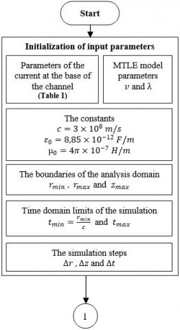
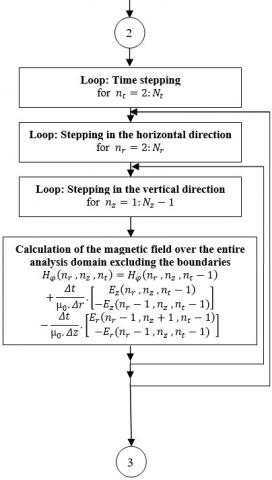
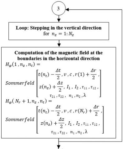
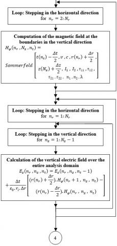
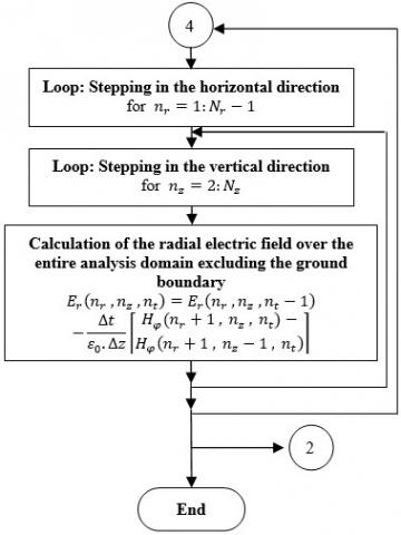
Based on the mathematical models described in the previous sections of this paper, which combine the accurate analytical formulation of Sommerfeld integrals at the domain boundaries with numerical processing inside the domain using the FDTD method, this section presents the main steps used to implement the proposed algorithm (Figure 3) within the MATLAB environment. These steps are as follows:
Figure 3. Algorithmic workflow of the hybrid approach
6.1 Initialization phase
The simulation begins with the initialization of all necessary parameters:
Input Parameters: These include the current waveform injected at the base of the lightning channel (as specified in Table 1, the parameters of the Modified Transmission Line with Exponential decay MTLE model, and relevant physical constants.
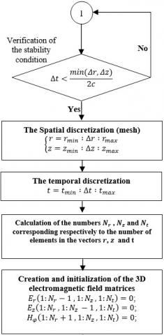
Spatial Discretization: The computational domain is discretized into a two-dimensional mesh along the radial r and vertical z axes. This meshing determines the resolution of the electromagnetic field components.
Temporal Discretization: The simulation time domain is defined, and the temporal step size $\Delta t$ is selected in accordance with stability criteria represented by Eq. (14).
Matrix Initialization: Three-dimensional matrices are created and initialized to store the electromagnetic field component $E_r(r, z, t)$, $E_z(r, z, t)$ and $H_{\varphi}(r, z, t)$.
Indexing Parameters: The number of discrete points along each axis $N_r$, $N_z$ and $N_t$ are computed to set the bounds of the iterative loops.
Stability Check: The condition given by Eq. (14) is verified to ensure numerical stability.
Table 1. Parameters of the current at the lightning channel base [38]
|
I1 (kA) |
τ11 (µs) |
τ12 (µs) |
n1 |
I2 (kA) |
τ21 (µs) |
τ22 (µs) |
n2 |
|
10.5 |
0.6 |
0.9 |
2 |
7 |
1.4 |
14 |
2 |
6.2 Time-stepping loop
A main loop iterates over each time step from t=0 to t=tmax. Within each time step, the following operations are performed sequentially:
6.3 Magnetic field computation
Interior Domain: The angular component of the magnetic field is updated over the entire analysis domain, excluding boundary cells. The update is based on Eq. (14).
Boundary Conditions: The subroutine named "Sommerfeld", which was previously developed, is invoked with all the required input parameters in order to compute the accurate numerical values of the magnetic field at the horizontal and vertical boundaries of the analysis domain. This subroutine performs its calculations based on Eqs. (15)-(17), and utilizes the numerical integration function quad provided by the MATLAB environment, as previously mentioned in an earlier section.
6.4 Vertical electric field computation
The vertical component of the electric field is updated across the full computational domain using Eq. (11), incorporating the effect of the magnetic field previously computed.
6.5 Radial electric field computation
The radial component of the electric field is calculated in all interior cells using Eq. (12), except for the cells located at the bottom boundary (ground interface), where the PEC condition is applied. This condition represents a perfectly conducting ground model, as described in Eq. (23).
6.6 Iteration
The algorithm loops over all spatial grid points in both radial and vertical directions at each time step. Once all components for the current time step are computed, the simulation advances to the next time level. This process continues until the entire temporal domain has been simulated.
This work presents a simulation of the electromagnetic field radiated by lightning, employing a hybrid strategy that blends the finite difference time domain technique and Sommerfeld integral techniques as absorbing boundary conditions.
To evaluate the scalability of the proposed approach, we conducted simulations with varying domain sizes and observation points. The computational complexity of the method primarily depends on the numerical evaluation of Sommerfeld integrals, which scales with FDTD. Compared to traditional FDTD with Mur’s ABC, our method significantly reduces the required memory by approximately 90%. Furthermore, the method exhibits better numerical stability for long-distance field calculations due to the elimination of artificial reflections at domain boundaries. The simulation, implemented in MATLAB, aimed to evaluate the accuracy and robustness of this hybrid method under simplified conditions.
Key parameters included observation distances of r=1 km and r=10 km, with a source height of z=5 m above a perfectly conductive ground. The electric and magnetic field components were analyzed at these observation points.
Results show that the hybrid approach minimizes boundary reflections more effectively than first-order Mur conditions, especially at greater distances. While the differences are negligible at r=1 km, significant improvements in stability and accuracy were observed at r=10 km. The assumption of perfectly conductive soil simplified the computations but may have led to an overestimation of field strength compared to realistic scenarios.
In the same context, a comparison was also conducted between the results obtained using the proposed method and experimental data available in the specialized literature. This comparison, carried out for waveforms recorded at distances of r=2 km, r=9 km and r=200 km from the lightning channel, showed good agreement between the two sets of results.
7.1 Observation point located 1 km from the canal
With the aim of highlighting some advantages of the approach for calculating the electromagnetic field radiated by lightning, which is based on a combination of the FDTD approach and Sommerfeld integral techniques used as absorbing boundary conditions, we decided to contrast the outcomes of this strategy with those of the identical FDTD method, but with first-order Mur absorbing boundary conditions. Through this comparison, we aim to demonstrate that bringing the vertical boundary of the analysis region closer to the observation point, as calculated by first-order Mur boundary conditions, introduces a significant error in the results. On the other hand, this proximity has an almost negligible impact when analytically calculated absorbing boundary conditions based on Sommerfeld integrals are used. This comparison was conducted in this work as follows:
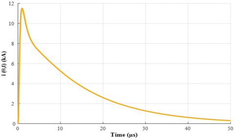
Figure 4 presents the time waveform of this current, which is characterized by a peak of 12 kA.
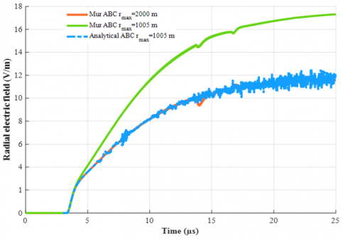
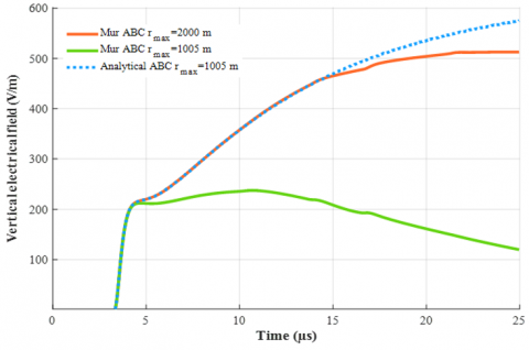
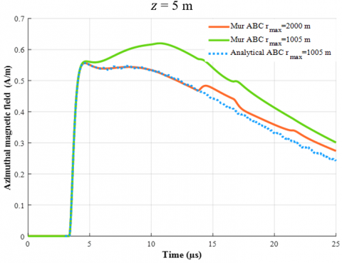
Figures 5-7 respectively show the waveforms of the radial electric field, vertical electric field and the azimuthal magnetic field evaluated at the observation point (r=1 km, z=5 m). To observe the effect of bringing the vertical boundary closer to this observation point, each of these waveforms was plotted again for the following three cases:
A boundary sufficiently far from the observation point to ensure good accuracy, placed at $r_{max }=2000 \mathrm{~m}$, and calculated using first-order Mur absorbing boundary conditions.
A boundary very close to the observation point, placed at $r_{max }=1005 \mathrm{~m}$, and calculated using first-order Mur absorbing boundary conditions.
In this work, the lightning channel is modeled using the MTLE approach, with a current propagation speed of $\mathrm{v}=0.8 \times 10^8 \mathrm{~m} / \mathrm{s}$ and a decay rate along the channel of λ=1 km. The current at the channel's base is represented as the sum of two Heidler functions, with parameters detailed in Table 1 [38].
Based on this comparison, assuming that the waveforms obtained for the first case, where a Mur's ABC is placed at $r_{max }=2000 \mathrm{~m}$, show good accuracy due to the ABC being sufficiently distant from the observation point, we can identify the significant error introduced in these waveforms when considering the second case with the ABC placed at $r_{max }=1005 \mathrm{~m}$.
This error is less pronounced for the magnetic field waveform since this component remains tangential at the analysis region boundaries. In contrast to the waveform behavior as the vertical boundary approaches the observation point, the curves obtained using boundary conditions calculated analytically through the numerical evaluation of Sommerfeld’s integrals maintain good accuracy, even when these absorbing boundary conditions are computed near the observation point.
Figure 4. Current at the channel's base
Figure 5. Radial electric field variation at r = 1 km and z = 5 m
Figure 6. Vertical electric field variation at r = 1 km and z = 5 m
Figure 7. Azimutal magnetic field variation at r = 1 km and z = 5 m
To better assess the improvement offered by the proposed hybrid method compared to the traditional Mur absorbing boundaries, we calculated the Root Mean Square Error (RMSE) and the total relative error (TRE) for both approaches at a selected observation point, based on the waveforms of the three field components $\mathrm{E}_{\mathrm{r}}, \mathrm{E}_{\mathrm{z}}$, and $\mathrm{H}_{\varphi}$, shown respectively in Figures 5-7. The calculations were performed using Eqs. (24) and (25), and the obtained results are summarized in Table 2.
Here, we assume that the time-domain waveforms obtained in the first case, where Mur’s ABC was placed at $\mathrm{r}_{\max }=2 \mathrm{~km}$, serve as the reference curves, since the absorbing boundary is located far enough to avoid reflections back to the observation point.
$R M S E=\sqrt{\frac{1}{n_{max }} \sum_{n=1}^{n_{max }}\left[W(n)-W_{r e f}(n)\right]^2}$ (24)
${TRE}(\%)=\frac{R M S E}{{Max}\left[W_{ {ref }}(n)\right]} \times 100$ (25)
where:
Wref(n): The reference instantaneous values of one of the components $E_r, E_z$, and $H_{\varphi}$.
W(n): The instantaneous values of one of the components $E_r, E_z$, and $H_{\varphi}$.
Table 2. Comparison of RMSE and the total relative error TRE between Mur’s ABC and Sommerfeld-based boundaries
|
W |
Method |
RMSE |
TRE (%) |
|
$E_r(\mathrm{V} / \mathrm{m})$ |
Mur ABC |
4.04 V/m |
27.47 |
|
Sommerfeld ABC |
0.35 V/m |
1.4 |
|
|
$E_z(\mathrm{V} / \mathrm{m})$ |
Mur ABC |
131.6 V/m |
27.83 |
|
Sommerfeld ABC |
2.16 V/m |
0.46 |
|
|
$H_{\varphi}(\mathrm{A} / \mathrm{m})$ |
Mur ABC |
0.06 A/m |
11.24 |
|
Sommerfeld ABC |
0.01 A/m |
1.88 |
These results (Table 2) clearly demonstrate that the absorbing boundary condition based on Sommerfeld integrals provides significantly higher accuracy, especially when the vertical boundary is located close to the observation point. In addition, computational resource usage was analyzed, and the results (as shown in Table 3) indicate that the proposed method achieves up to 90% memory savings compared to Mur’s approach, confirming its efficiency for large-scale simulations.
Therefore, we can conclude that this method for calculating the electromagnetic field radiated by lightning possesses a distinctive advantage not found in Mur's ABCs: It ensures high accuracy even for nodes located near the boundaries of the analysis region.
7.2 Observation point located 10 km from the canal
The objective here is to demonstrate that the advantages of this approach become particularly evident when focusing on long distances. This is reflected mainly in a significant reduction in memory use and, consequently, in computation time. This improvement is due to the fact that it is not necessary to mesh the analysis region up to the lightning channel. This calculation method allows the lightning channel to be replaced by magnetic field values obtained on a lower vertical boundary using Sommerfeld integrals.
In this context, we used our MATLAB calculation code, developed for this work and based on this approach, to plot Figures 8 and 9, which respectively present the waveforms of the vertical electric field and the azimuthal magnetic field evaluated at the observation point (r=10 km, z=5 m).
Figure 8. Vertical electric field variation at r=10 km, z=5 m
Figure 9. Azimutal magnetic field variation at r=10 km, z=5 m
For comparison, we also plotted on each of these two figures the waveforms obtained by adopting first-order Mur boundary conditions. We can clearly observe in both figures what is likely a superposition of a numerically reflected wave through Mur boundary conditions, unlike the patterns obtained using Sommerfeld integrals. This is one of the advantages of this approach.
Thus, Table 3 illustrates a comparison of matrix sizes involved in the calculations for the two cases mentioned above (FDTD + Mur ABC and FDTD + Sommerfeld ABC). The comparison was made for each component of the radiated electromagnetic field.
Table 3. Matrix sizes of three electromagnetic field components used in the calculation
|
Cases |
Er |
Ez |
Hφ |
|
ABC of Mur |
2000×801×10001 |
2001×800×10001 |
2001×801×10001 |
|
ABC of Sommerfeld |
400×201×4001 |
401×200×4001 |
402×201×4001 |
We can observe from this comparison a significant reduction in matrix sizes when using the FDTD approach with Sommerfeld ABC. This reduction reaches 90% of the memory space used compared to the same FDTD method with Mur ABC. This represents a major advantage of this approach for studying the far-field radiated electromagnetic field generated by lightning.
In this study, we assume a perfectly conducting ground to simplify the computation of electromagnetic fields. However, real ground conditions involve varying conductivities, which can significantly impact field propagation. Future work will extend our model to consider finitely conducting ground using more complex Sommerfeld integral formulations. Incorporating multi-layer soil conductivity models or using experimental validation from field measurements will enhance the realism and applicability of this approach.
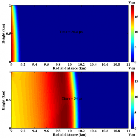
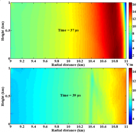
Using the numerical code developed in this research, we were able to generate time-evolving maps of the vertical electric field, providing a more comprehensive and clearer representation of the results.
It is important to note that the analysis area was defined by the following spatial limits: $r_{\min }=9 \mathrm{~km}$ and $r_{\max }=11 \mathrm{~km}$ for the vertical dimension, as well as $z_{\text {min }}=0$ and $z_{\text {max }}=$ 1 km for the horizontal dimension. The temporal range of the study extended from $t_{\min }=30 \,\, \mu s$ to $t_{\max }=50 \,\, \mu s$.
In this study, we present some excerpts from these maps for the moments 30.6, 34, 37, and 39 µs (see Figure 10).
The analysis of these results allows us to formulate the following observations:
1- The emergence of a vertical electric field wave through the lower vertical boundary of the analysis region ($r_{min }=9 \mathrm{~km}$) at t=30.6 µs demonstrates that the approach used in this work to compute this field, unlike traditional absorbing boundary conditions, enabled the wave to penetrate the analysis region. This occurred despite the lightning channel— the source of the electric field— being located outside this region. This characteristic is a major advantage of the proposed approach, as it allows for flexible reduction of the analysis region based on simulation requirements, without the constraint of defining it relative to the lightning channel, as is necessary with conventional absorbing boundaries.
Figure 10. The time-evolving maps of the vertical electric field
2- The vertical electric field wave propagates within the analysis region (at t=34 µs) without any distortion in the boundaries between its different levels caused by non-physical reflections. This demonstrates that the approach used in this study effectively prevents such reflections.
3- The vertical electric field wave begins to exit the analysis area at t=37 µs through the maximum vertical boundary $r_{max }=11 \mathrm{~km}$ smoothly, without any distortions in the separation lines between its different levels, despite being near this boundary. This reinforces the findings from Figures 4-6, highlighting the effectiveness of the proposed boundary type in this research, particularly in regions close to the boundary.
4- The wave fully exits the analysis area at t=39 µs, confirming that the vertical electric field values inside the area remain unaffected by any reflections that could introduce significant calculation errors.
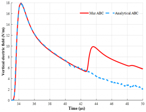
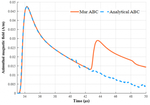
7.3 Experimental validation
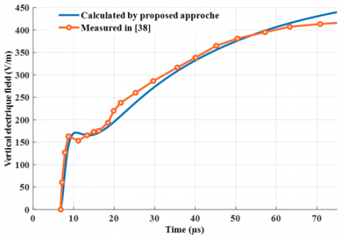
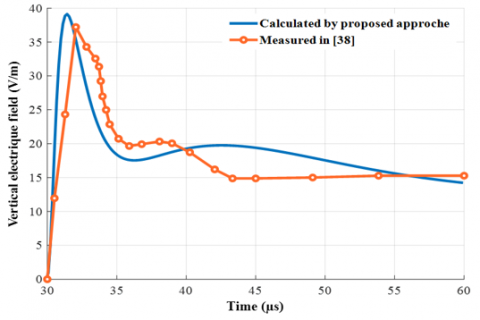
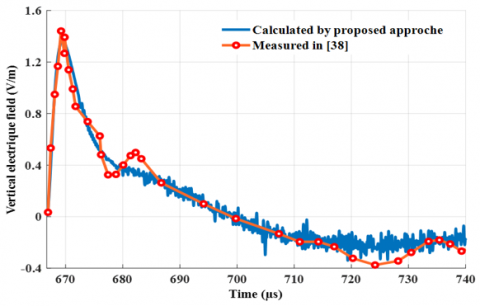
The developed computational code was experimentally validated by comparing simulation results obtained using our implementation of the proposed approach with measurement data reported in reference [38], collected during an experimental campaign conducted in August 1987 at the Kennedy Space Center in Florida. This comparison (see Figures 11-13) reveals a good agreement between the waveforms calculated and those obtained from the experimental measurements at the Kennedy Space Center [38].
Additionally, we would like to point out that the simulation results clearly demonstrated the most prominent characteristics of both the near and far electromagnetic fields, which have been reported by many researchers specialized in this field [39]. The electromagnetic field exhibits, at all distances (between 1 km and 200 km), an initial peak whose intensity is approximately inversely proportional to the distance. At relatively close distances, the electric field shows a gradual decay following the initial peak. As for the distant electric and magnetic fields (at distances greater than approximately 50 km), they essentially share the same waveform and exhibit a polarity reversal a phenomenon known as polarity inversion in the far field, which is considered one of the most distinctive features of such fields the polarity reversal phenomenon in the far-field, which is considered one of the most distinctive characteristics of such fields.
Figure 11. Vertical electric field variation at r = 2 km
Figure 12. Vertical electric field variation at r = 9 km
Figure 13. Vertical electric field variation at r = 200 km
It can also be observed in Figure 13 that there are some minor high-frequency reflections in the tail of the waveform; however, they did not significantly affect the overall shape of the wave. The appearance of these reflections is attributed to the reduced size of the analysis domain, as well as the large time window used relative to the capabilities of the available basic numerical tools, considering the computational load required.
In this study, we applied our previously proposed hybrid approach [9], combining the FDTD method and Sommerfeld integrals, to compute the far-field electromagnetic radiation of lightning over a perfectly conducting ground. Our objective was to reduce memory usage while maintaining accuracy in large-scale computations. The results demonstrate a significant decrease in allocated memory space, confirming the efficiency of the method for far-field electromagnetic field mapping.
Despite the promising results, further improvements can be explored. Future work could focus on extending the approach to more complex ground conditions, such as finitely conducting or stratified media, to enhance realism. Additionally, optimizing the algorithm for three-dimensional simulations could provide a more comprehensive understanding of lightning-induced electromagnetic effects.
Another avenue for development is the parallelization of computations to further improve efficiency and reduce execution time. Integrating machine learning techniques for adaptive meshing and optimization could also enhance computational performance. These improvements would make the method more suitable for real-time applications in lightning protection, electromagnetic compatibility studies, and geophysical investigations.
We sincerely appreciate everyone who dedicated their time and efforts, both directly and indirectly, to the successful completion of our project as part of our curriculum. We are also deeply grateful to the Electrical Engineering Department for its invaluable support and resources.
|
E |
Electric field |
|
Er |
Radial (horizontal) component of electric field |
|
Ez |
Vertical component of electric field thermal |
| H | Magnetic field |
|
Hϕ |
Azimuthal magnetic field component |
|
I |
Peak current (Heidler function parameter) |
|
i(z, t) |
Lightning return stroke current distribution in time and space |
|
v |
Propagation speed of lightning current along the channel |
|
c |
Speed of light |
|
Greek symbols |
|
|
$\varepsilon$ |
Permittivity (F/m) |
|
$\mu$ |
Permeability (H/m) |
|
$\sigma$ |
Electrical conductivity (S/m) |
|
$\lambda$ |
Attenuation factor of current along the channel (1/m) |
|
$\eta$ |
Exponential factor in Heidler function |
|
$\tau_1, \tau_2$ |
Front and tail time constants (µs) |
|
Subscripts |
|
|
r |
Radial or horizontal direction |
|
z |
Vertical direction (elevation) |
|
ϕ |
Azimuthal direction (angular) |
[1] Rachidi, F., Nucci, C.A., Ianoz, M., Mazzetti, C. (2002). Influence of a lossy ground on lightning-induced voltages on overhead lines. IEEE Transactions on Electromagnetic Compatibility, 38(3): 250-264. https://doi.org/10.1109/15.536054
[2] Rubinstein, M. (1996). An approximate formula for the calculation of the horizontal electric field from lightning at close, intermediate, and long range. IEEE Transactions on Electromagnetic Compatibility, 38(3): 531-535. https://doi.org/10.1109/15.536087
[3] Zeddam, A., Degauque, P. (2017). Current and voltage induced on telecommunication cables by a lightning stroke. In Lightning Electromagnetics. Routledge, pp. 377-400. https://doi.org/10.1080/02726348708908197
[4] Uman, M.A. (2001). The lightning discharge. Physics Today, 42(5): 75-76. https://doi.org/10.1063/1.2811019
[5] Leteinturier, C. (1980). Champ électromagnétique émis par une décharge orageuse: Modèle théorique intégrant les variations de la résistivité du sol. Doctoral dissertation.
[6] Liu, X., Ge, T. (2020). An efficient method for calculating the lightning electromagnetic field over perfectly conducting ground. Applied Sciences, 10(12): 4263. https://doi.org/10.3390/app10124263
[7] Arzag, K., Ghemri, B., Azzouz, Z.E. (2018). Lightning electric and magnetic fields computation using the 3D-FDTD method and electromagnetic models in presence of different ground configurations. IEEJ Transactions on Power and Energy, 138(5): 315-320. https://doi.org/10.1541/ieejpes.138.315
[8] La Fata, A., Nicora, M., Mestriner, D., Aramini, R., Procopio, R., Brignone, M., Delfino, F. (2023). Lightning electromagnetic fields computation: A review of the available approaches. Energies, 16(5): 2436. https://doi.org/10.3390/en16052436
[9] Habri, K., Azzouz, Z., Mimouni, A. (2019). Hybridization between the FDTD method and sommerfeld integrals for lightning electromagnetic field calculation. In 2019 International Conference on Advanced Electrical Engineering (ICAEE), Algiers, Algeria, pp. 1-8. https://doi.org/10.1109/ICAEE47123.2019.9015116
[10] Arzag, K., Azzouz, Z.E., Baba, Y. (2019). 3D-FDTD computation of lightning electromagnetic fields in the presence of a mountain and a river. In 2019 International Symposium on Lightning Protection (XV SIPDA), Sao Paulo, Brazil, pp. 1-6. https://doi.org/10.1109/SIPDA47030.2019.8951698
[11] Kohlmann, H. (2020). FDTD simulation of lightning electromagnetic fields: An approach with the software package MEEP. Diploma thesis, Technische Universität Wien. https://doi.org/10.34726/hss.2020.65348
[12] Makarov, P.A., Ustyugov, V.A. (2024). Features of numerical solution of the maxwell equations by the FDTD method in the homogeneous and inhomogeneous formulations. Technical Physics, 69(8): 2227-2240. https://doi.org/10.1134/S1063784224700543
[13] Zhang, G., Chen, M., Wang, S., Gao, Y., Du, Y.P. (2023). A new FDTD model for lightning return stroke channel above lossy ground and its validation with rocket-triggered lightning data. IEEE Access, 11: 84475-84486. https://doi.org/10.1109/ACCESS.2023.3303478
[14] Mimouni, A. (2007). Electromagnetic environment in the immediate vicinity of a lightning return stroke. Journal of Lightning Research, 2: 64-75.
[15] Mimouni, A. (2007). Analyse des problèmes de compatibilité électromagnétique par modélisation et simulation du rayonnement électromagnétique de la foudre. Université desSciences and Technologies Oran Mohamed Boudiaf.
[16] Yee, K. (1966). Numerical solution of initial boundary value problems involving Maxwell's equations in isotropic media. IEEE Transactions on Antennas and Propagation, 14(3): 302-307. https://doi.org/10.1109/TAP.1966.1138693
[17] Jiang, L., Dong, X., Zhou, X., Wang, J., Song, J., Ma, Q. (2023). Propagation characteristics of lightning radiation field on three-layer vertical layered ground based on cpml absorption boundary. IEEE Transactions on Electromagnetic Compatibility, 65(4): 1191-1201. https://doi.org/10.1109/TEMC.2023.3268311
[18] Padilla-Perez, D., Medina-Sanchez, I., Hernández, J., Couder-Castaneda, C. (2022). Accelerating electromagnetic field simulations based on memory-optimized CPML-FDTD with OpenACC. Applied Sciences, 12(22): 11430. https://doi.org/10.3390/app122211430
[19] Zhang, Z., Tian, Y., Wang, C., Wang, X., Tian, Y. (2021). Lightning return stroke electromagnetic field and energy at close distance by using 3D FDTD simulation. International Journal of Applied Electromagnetics and Mechanics, 65(2): 215-233. https://doi.org/10.3233/JAE-190133
[20] Chahmi, A., Birane, M. (2022). Contribution to the analysis of the electromagnetic field radiated by lightning taking into account the conductivity of the ground. In 2022 International Conference of Advanced Technology in Electronic and Electrical Engineering (ICATEEE), M'sila, Algeria, pp. 1-5. https://doi.org/10.1109/ICATEEE57445.2022.10093740
[21] Fan, X., Zhang, Y., Krehbiel, P.R., Zhang, Y., Zheng, D., et al. (2020). Application of ensemble empirical mode decomposition in low-frequency lightning electric field signal analysis and lightning location. IEEE Transactions on Geoscience and Remote Sensing, 59(1): 86-100. https://doi.org/10.1109/TGRS.2020.2991724
[22] M'ziou, N., Mokhnache, L., Boubakeur, A., Azzouz, Z., Kattan, R. (2010). Computation of lightning electromagnetic field in the presence of a tall tower with the HYBRID method. COMPEL-The International Journal for Computation and Mathematics in Electrical and Electronic Engineering, 29(4): 930-940. https://doi.org/10.1108/03321641011044343
[23] Elcherbeni, A.Z., Demir, V. (2015). The Finite-Difference Time-Domain Method for Electromagnetics with MATLAB Simulation (2nd ed.). SciTech Publishing.
[24] Inan, U.S., Marshall, R.A. (2011). Numerical Electromagnetics: The FDTD Method. Cambridge University Press.
[25] Arzag, K., Azzouz, Z.E., Ghemri, B. (2016). 3D-FDTD computation of lightning return stroke current and associated electromagnetic field using electromagnetic models. International Review of Electrical Engineering (IREE), 11(5): 517. https://doi.org/10.15866/iree.v11i5.9697
[26] Berenger, J.P. (1994). A perfectly matched layer for the absorption of electromagnetic waves. Journal of Computational Physics, 114(2): 185-200. https://doi.org/10.1006/jcph.1994.1159
[27] Ramahi, O.M. (1997). Complementary boundary operators for wave propagation problems. Journal of Computational Physics, 133(1): 113-128. https://doi.org/10.1006/jcph.1997.5658
[28] Rudolph, T., He, T., Sherman, B.D., Nozari, B. (1995). Low frequency boundary condition for the time domain finite difference technique. In Proceedings of International Symposium on Electromagnetic Compatibility, Atlanta, GA, USA, pp. 163-167. https://doi.org/10.1109/ISEMC.1995.523539
[29] Mur, G. (2007). Absorbing boundary conditions for the finite-difference approximation of the time-domain electromagnetic-field equations. IEEE Transactions on Electromagnetic Compatibility, 4: 377-382. https://doi.org/10.1109/TEMC.1981.303970
[30] McCoy, D.E., Shneidman, A.V., Davis, A.L., Aizenberg, J. (2021). Finite-difference time-domain (FDTD) optical simulations: A primer for the life sciences and bio-inspired engineering. Micron, 151: 103160. https://doi.org/10.1016/j.micron.2021.103160
[31] Ghania, S.M. (2023). Electromagnetic transients around power lines using FDTD method. Engineering, Technology & Applied Science Research, 13(6): 12.
[32] Xiang, Y., Rao, P., Feng, W., Ouyang, B. (2024). Evaluation of temporal distribution of lightning electromagnetic field in inhomogeneous soil. Acta Geophysica, 72: 793-805. https://doi.org/10.1007/s11600-023-01100-w
[33] Brignone, M., Procopio, R., Nicora, M., Mestriner, D., Rachidi, F., Rubinstein, M. (2022). A Prony-based approach for accelerating the lightning electromagnetic fields computation above a perfectly conducting ground. Electric Power Systems Research, 210: 108125. https://doi.org/10.1016/j.epsr.2022.108125
[34] Cooray, V., Cooray, G., Rubinstein, M., Rachidi, F. (2023). Exact expressions for lightning electromagnetic fields: Application to the Rusck field-to-transmission line coupling model. Atmosphere, 14(2): 350. https://doi.org/10.3390/atmos14020350
[35] Li, D., Luque, A., Rachidi, F. (2022). Application of the finite-difference time-domain (FDTD) technique in lightning studies. In Advanced Time Domain Modeling for Electrical Engineering. https://doi.org/10.1049/SBEW550E_ch11
[36] Nucci, C.A., Mazzetti, C., Rachidi, F., Ianoz, M. (1988). Analyse du champ électromagnétique dû à une décharge de foudre dans les domaines temporel et fréquentiel. Annales des Télécommunications, 43(11): 625-637. https://doi.org/10.1007/BF02995262
[37] Heidler, F. (1985). Analytic lightning current functions for LEMP calculations. In 18th International Conference on Lightning Protection (ICLP), VDE Verlag, Berlin, West Germany, pp. 63-66.
[38] Orzan, D. (1998). Couplage interne et externe entre un champ électromagnétique et un réseau de lignes multifilaires. Doctoral dissertation, École Polytechnique Fédérale de Lausanne.
[39] Lin, Y.T., Uman, M.A., Tiller, J.A., Brantley, R.D., Beasley, W.H., Krider, E.P., Weidman, C.D. (1979). Characterization of lightning return stroke electric and magnetic fields from simultaneous two-station measurements. Journal of Geophysical Research: Oceans, 84(C10): 6307-6314. https://doi.org/10.1029/JC084iC10p06307