Boyun Guo*![]() | Yin Feng
| Yin Feng![]() | Sohail Nawab
| Sohail Nawab![]()
© 2025 The authors. This article is published by IIETA and is licensed under the CC BY 4.0 license (http://creativecommons.org/licenses/by/4.0/).
OPEN ACCESS
Production forecasting in hydraulic-fractured shale reservoirs requires reliable mathematical models that capture the coupled flow between fractures and the surrounding rock matrix. This study develops an analytical solution for distributed cross-flow (DCF) in a shale reservoir by formulating and solving a differential-integral equation that accounts for pressure evolution under varying boundary conditions. The analysis is based on two key assumptions: (1) the study focuses on the steady-state and pseudo-steady-state regimes, when boundary effects dominate; and (2) the model assumes flow along the x-direction inside the fracture and flow in the y-direction from the matrix to the fracture, while horizontal flow within the matrix is neglected. These assumptions enable a tractable yet insightful formulation of fluid movement from the shale matrix to the fracture network. The analytical approach provides explicit expressions for pressure and flow distributions, allowing rapid evaluation of production scenarios without reliance on heavy numerical simulations. Results show that under a no-flow boundary condition, the cumulative fluid rate is initially higher but declines with time due to reservoir depletion, whereas constant-pressure boundaries maintain a steady flux. The framework offers both physical clarity and practical advantages, including computational efficiency, straightforward sensitivity analysis, and adaptability for integration into larger reservoir models.
shale reservoir, hydraulic fracture, well productivity, distributed cross-flow, differential-integral equation
1.1 Background
The development of shale oil and gas resources through horizontal drilling and multi-stage hydraulic fracturing has transformed the global energy landscape, enabling production from formations once considered uneconomic. Hydraulic fractures act as highly conductive flow conduits, connecting ultra-tight shale matrix systems (often with nano-Darcy-level permeability) to the wellbore. This connectivity is critical to production performance, but the prediction of well productivity relies on accurately modeling how fluids migrate from the matrix through complex fracture networks.
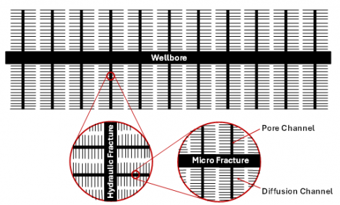
Shale formations are inherently heterogeneous and hierarchical. Figure 1 depicts the fractal structure of fluid flow in a hydraulically fractured shale reservoir: (i) at the highest level, fluids flow from hydraulic fractures into the wellbore; (ii) at the next level, microfractures feed into the main hydraulic fractures; (iii) at a finer scale, fluids flow from pore channels into microfractures; and (iv) at the smallest scale, diffusion occurs from the matrix solid into the pore network. These four levels are presented as a conceptual hierarchy because they correspond to commonly observed flow domains reported in core studies, microseismic analyses, and lab-scale imaging. Each level is controlled by distinct mechanisms: matrix-to-pore exchange is dominated by diffusion and capillarity; pore-to-microfracture transfer is governed by capillary imbibition and viscous resistance; microfracture-to-fracture flow occurs under pressure-driven Darcy flow; and fracture-to-wellbore flow is controlled by high-conductivity fracture transport. This “four-level” representation is scalable: depending on data resolution and rock type, the hierarchy can collapse into fewer levels or expand to include nanopores within kerogen or natural fractures intersecting the hydraulic network.
Figure 1. Fractal presentation of fluid flow in hydraulic-fractured shale reservoirs
Distributed cross-flow (DCF) is not unique to shale reservoirs. Similar phenomena occur in particle filtration systems, water movement in unconfined aquifers, and multiphase flow in heterogeneous reservoirs. In this study, we use DCF analogies selectively and explicitly tie them to shale processes. For example, in cross-flow membrane filtration, the buildup of a fouling layer is conceptually similar to microfracture plugging in shale, where the “sub-stream” (pore-scale flow) faces increasing restriction. Likewise, heat exchangers provide analytical frameworks for cross-flow transfer that mirror the pressure-driven coupling between the shale matrix and fracture system. These analogies are used not as unrelated examples, but to illustrate how restrictive cross-domain transfer in shale can be captured analytically. What distinguishes shale, however, is the extreme restriction on sub-stream flow at multiple levels: the transition from matrix to pore channels, from pore channels to micro fractures, and so forth. Each transition is influenced by capillary forces, viscous resistance, and sometimes gravity segregation, creating a cascade of restrictive flows. This complex interplay means that modeling shale production is not simply a matter of simulating flow through fractures as it requires understanding how each restrictive DCF interface contributes to overall system behavior.
A variety of approaches have been developed to characterize and model flow in hydraulically fractured shale reservoirs. The literature can be grouped into three major areas: fracture characterization, modeling approaches, and DCF research.
2.1 Fracture characterization
Microseismic monitoring with geophones has been widely used to track the propagation and geometry of hydraulic fractures during stimulation treatments [1, 2]. Microseismic data reflect the locations of rock failure events inside shale formations and have revealed that event source points rarely follow planar geometries in three-dimensional space, indicating significant fracture path variability [1]. Warpinski [2] reported microseismic data suggesting fracture propagation trends perpendicular to the horizontal wellbore, though no definitive fracture configuration was derived.
Building on microseismic imaging, Abdulaziz [3] mapped hierarchical fracture branches in the Barnett Shale, while Barati and Liang [4] assumed hydraulic fractures with lateral branches in their fracturing fluid system design. Li and Zhang [5] presented a fracture network model incorporating fracture complexity, and Feng et al. [6] analyzed factors influencing fracture system complexity based on energy conservation principles. Other researchers have focused on the intersection of induced fractures with natural microfractures, forming hybrid or tree-like networks [7-10]. Post-fracturing studies further confirmed complex fracture evolution and reactivation processes [11, 12].
While these studies have greatly advanced understanding of fracture morphology, the mechanism of oil flow in hydraulically fractured shale remains a topic of debate. Observations from microseismic data, laboratory experiments, and field studies are often reconciled by building mathematical models that “fit” production history through parameter tuning, rather than deriving relationships grounded in first principles. This practice makes it challenging to distinguish whether a model’s accuracy reflects true physical understanding or merely calibration flexibility.
2.2 Modeling approaches
Classic analytical fracture models laid the foundation for modern shale reservoir modeling. Warren and Root’s dual-porosity model [13] first formalized the concept of matrix–fracture fluid exchange, while Cinco-Ley and Samaniego-V [14] provided semi-analytical solutions for finite- and infinite-conductivity fractures that remain widely used. Gringarten et al. [15] expanded these approaches to include transient flow, setting the stage for decades of analytical and semi-analytical studies. Building on these foundations, more recent research has incorporated discrete fracture network (DFN) modeling [16] and stimulated reservoir volume (SRV) concepts to represent fracture complexity at field scale. Recent works have also explored hybrid physics–data approaches for production forecasting (e.g., references [17, 18]), integrating physics-based understanding with machine learning to improve prediction accuracy.
A broad range of modeling strategies have been developed to describe flow in fractured shales, ranging from empirical decline curve methods to fully numerical simulators. Hyman et al. [19] conceptualized production decline in three distinct flow stages (fracture-dominated, damaged zone, and matrix contribution) providing a useful qualitative framework. Dai et al. [20] applied semi-analytical models assuming fractal fracture networks, capturing some of the hierarchical features revealed by microseismic data. Hu et al. [21] advanced the field by creating discrete fracture network (DFN)–based models for gas production, explicitly incorporating fracture geometry. Despite these contributions, many models remain heavily numerical in nature, requiring extensive tuning of poorly constrained parameters (e.g., fracture conductivity, stimulated reservoir volume) to match production histories. Such models often obscure underlying physics and provide limited insight into scaling relationships or sensitivity trends.
2.3 DCF research
The flow between the shale matrix and fractures conceptually falls into the broader category of DCF, defined as mass transfer between domains driven by a potential gradient. In shale systems, this includes flow from matrix to pores, pores to microfractures, and microfractures to hydraulic fractures, each representing a level of restricted DCF. DCF phenomena have been well studied in other engineering disciplines, including filtration, aquifer flow, and heat transfer, offering valuable analogies for shale modeling. For example, Huisman [22] reviewed early work on membrane separations and microfiltration; Ferreira and Massarani [23] developed a phenomenological model correlating pressure fields, filtration rates, and cake thickness in axial cross-flow filtration; and Hakami et al. [24] investigated ceramic membrane microfiltration for wastewater treatment, focusing on fouling and flow restriction. More recent reviews (e.g., reference [25]) on microalgal dewatering further highlight the importance of DCF in particle filtration systems.
Other studies moved beyond empirical work into numerical and semi-analytical territory. Kazemi et al. [26] conducted numerical simulations of cross-flow microfiltration of diluted malt extract suspensions by tubular ceramic membranes, showing strong agreement with experimental data—but the discretized nature of their solution makes it difficult for practitioners to use directly. Park and Nägele [27] presented an analytical model for ultrafiltration of permeable particle dispersions in hollow fiber membranes, using a semi-analytic modified boundary layer approximation. Parasyris et al. [28] extended similar concepts to circular filtration modules. While useful, these works either over-simplified the coupling between mainstream and sub-stream flow or ignored sub-stream flow restriction—a critical feature of shale systems.
DCF research in heat transfer also offers partial parallels. Bradley [29] presented simplified analytical treatments for counterflow, crossflow, and concurrent-flow heat exchangers. More recently, Liu et al. [30] developed a distributed parameter model for plate-fin heat exchangers (PFHEs) to investigate counterflow and cross-flow thermodynamics, including the effect of longitudinal conduction. However, none of these studies, across filtration, aquifer, or heat transfer literature, address the analytical modeling of restrictive DCF systems where the sub-stream is strongly coupled to, and constrained by, the mainstream flow.
2.4 Knowledge gaps
Despite decades of research, analytical modeling of flow in fractured shale systems remains underdeveloped. The industry relies heavily on numerical simulation tools such as dual-porosity and dual-permeability models, which can handle heterogeneity and multiphase effects but are computationally demanding and often obscure the underlying physics. For many engineers, these models are essentially “black boxes” offering little insight into sensitivity trends or scaling behavior. While the DCF concept is widely recognized in other engineering disciplines, shale applications have few (if any) analytical treatments that capture both fracture flow and matrix contribution in a single, closed-form framework. In shale, the “sub-stream” (e.g., fluid flow from matrix or microfractures) is highly restricted and tightly coupled to the “mainstream” flow within hydraulic fractures. Representing this interdependency analytically is challenging. In most cases, systems must be discretized, and numerical methods are used approaches that can be inaccessible to field engineers and obscure physical interpretation. The pseudo-steady-state period when reservoir boundaries begin to influence pressure and production behavior, is critical for production forecasting and decline analysis. Yet very few studies explicitly analyze how constant-pressure versus no-flow boundaries affect flow evolution and flux partitioning in shale systems. Existing analytical studies often focus on a single scale (e.g., matrix to fracture) and do not explicitly account for the cascading nature of DCF from pore channels up to fractures and then to the wellbore.
2.5 Objectives
This study aims to fill these gaps by developing an analytical solution for DCF between the shale matrix and hydraulic fractures using a differential–integral equation (DIE) formulation. The solution is derived under two simplifying but physically meaningful assumptions: (1) the analysis focuses on the pseudo-steady-state regime; and (2) flow is assumed to occur along the fracture in the x-direction and from the matrix in the y-direction, neglecting horizontal flow within the matrix. By incorporating these assumptions, we derive closed-form expressions for pressure and flow distributions under both constant-pressure and no-flow boundaries. This analytical framework provides a transparent and computationally efficient alternative to purely numerical simulations, offering both conceptual clarity and practical utility for reservoir engineers.
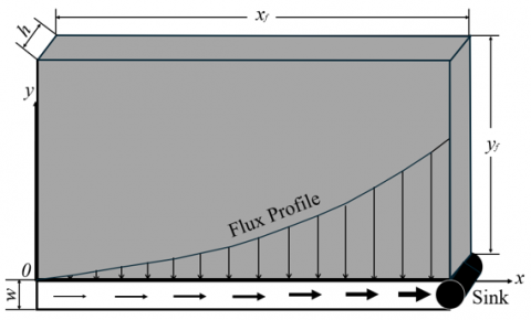
Mass or heat DCF in a 2-dimentional domain is depicted in Figure 2. The DIE method used in this study involves the following procedure:
Define the flux function in the 2D-domain based on physics law (e.g., Darcy’s law for fluid flow in porous media or Fourier’s law for heat conduction):
$q_y(x, 0)=a \frac{h \Delta x}{y_f}\left[\Phi\left(x, y_f\right)-\Phi(x, 0)\right]$ (1)
where, $q(x, 0)$ is the flow rate, $\Phi$ is potential function, $a$ is constant, and other quantities are shown in Figure 3.
Figure 2. Mass or heat DCF in a 2-dimentional domain
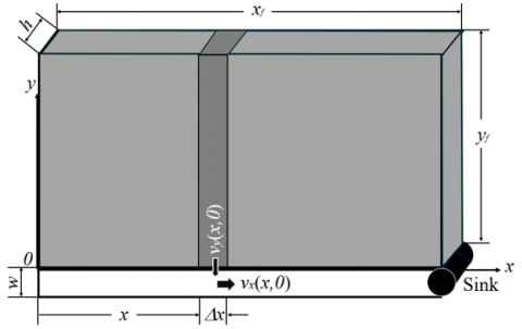
Figure 3. Velocities at the joint of DCF in a 2-dimentional domain
Formulate the flux velocity in y-direction at x by dividing flow rate by flow cross-sectional area:
$v_y(x, 0)=\frac{a}{y_f}\left[\Phi\left(x, y_f\right)-\Phi(x, 0)\right]$ (2)
Formulate the flow rate in x-direction at x-point by integrating the influx from x=0 to x:
$q_x(x, 0)=\frac{a h}{y_f} \int_0^x\left[\Phi\left(x, y_f\right)-\Phi(x, 0)\right] d x$ (3)
Formulate the flux velocity in x-direction at x by dividing flow rate by flow cross-sectional area of the mainstream:
$v_x(x, 0)=\frac{\mathrm{a}}{w y_f} \int_0^x\left[\Phi\left(\mathrm{x}, y_f\right)-\Phi(\mathrm{x}, 0)\right] d x$ (4)
Formulate the velocity in x-direction at x in the mainstream based on physics law (e.g., Darcy’s law for fluid flow in porous media or Fourier’s law for heat conduction):
$v_x(x, 0)=-b \frac{d \Phi(x, 0)}{d x}$ (5)
The velocity at point x must be unique. Therefore, the right sides of Eq. (4) and Eq. (5) must be equal, i.e.,
$\frac{a}{w y_f} \int_0^x\left[\Phi\left(x, y_f\right)-\Phi(x, 0)\right] d x=-b \frac{d \Phi(x, 0)}{d x}$ (6)
which is a differential-integration equation to solve.
Taking derivative of Eq. (6) with respect to $x$ gives:
$\frac{a}{w y_f}\left[\Phi\left(x, y_f\right)-\Phi(x, 0)\right]=-b \frac{d^2 \Phi(x, 0)}{d x^2}$ (7)
Solve Eq. (7) with boundary conditions for the potential function $\Phi(x, 0)$.
Submit the potential function back to Eq. (3) and integrate the latter will allow for determination of the influx profile function.
The total influx at the sink is obtained by integrating the influx function from $x=0$ to $x=x_f$, i.e.,
$q_x\left(x_f, 0\right)=\frac{a h}{y_f} \int_0^{x_f}\left[\Phi\left(x, y_f\right)-\Phi(x, 0)\right] d x$ (8)
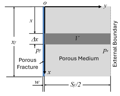
Figure 4. Fluid DCF from a porous medium to a fracture of finite conductivity
Figure 4 depicts fluid DCF from a porous medium to a porous fracture in a horizontal plane. Only crossflow on one side of the fracture is shown due to symmetry. If the external boundary is a no-flow boundary, consider the fluid in a volume element V flowing to the fracture. The fluid volume is expressed as:
$V=\frac{1}{2} \phi h S_f \Delta x$ (9)
where, $\phi$ is porosity, $h$ is the thickness of the flow domain, $S_f$ is the length of the flow domain, and $\Delta x$ is the width of the element $V$.
The governing equation for fluid flow in the porous medium is:
$\frac{\partial^2 p}{\partial y^2}=\frac{\phi \mu C}{k_m} \frac{\partial p}{\partial t}$ (10)
where, $p$ is pressure, $\mu$ is fluid viscosity, $C$ is fluid compressibility, $k_m$ is permeability, and $t$ is time.
3.1 Solution under constant-pressure boundary condition
The constant-pressure boundary creates a steady flow, i.e., $\partial p / \partial t=0$. Then Eq. (10) degenerates to:
$\frac{\partial^2 p}{\partial y^2}=0$ (11)
or
$\frac{\partial p}{\partial y}=c_0$ (12)
where, $c_0$ is a constant and according to Darcy's law, $c_0= \frac{\mu q(x)}{k_m h \Delta x}$.
$q(x)=\frac{k_m h \Delta x}{\mu} \frac{\partial p}{\partial y}$ (13)
which is integrated to get:
$p=\frac{\mu}{k_m h \Delta x} q(x) y+c_0^{\prime}$ (14)
The inner boundary condition is:
$\left.p\right|_{y=0}=p_f(x)$ (15)
which is applied to Eq. (14) to give:
$c_0^{\prime}=p_f(x)$ (16)
Substituting Eq. (16) into Eq. (14) and evaluating the latter at the outer boundary where $y=\frac{S_f}{2}$ gives:
$p_e=\frac{\mu S_f}{2 k_m h \Delta x} q(x)+p_f(x)$ (17)
which is arranged to get:
$q(x)=\frac{2 k_m h \Delta x}{\mu S_f}\left[p_e-p_f(x)\right]$ (18)
Note that segment flow rate $q(x)$ as shown in Eq. (18) only considers inflow from a single fracture face and to account for both fracture faces, the rate must be multiplied by two.
3.2 Solution under no-flow boundary condition
The fluid compressibility is defined as:
$C=-\frac{1}{V}\left(\frac{\partial V}{\partial p}\right)$ (19)
which is divided by dt and rearranged to get
$C V \frac{\partial p}{\partial t}=-\frac{\partial V}{\partial t}=-q(x)$ (20)
where, $q(x)$ is the volumetric flow (flux) rate at point $x$. Substituting Eq. (9) into Eq. (20) gives:
$\frac{\partial p}{\partial t}=-\frac{q(x)}{C V}=-\frac{2 q(x)}{C \phi h S_f \Delta x}$ (21)
which is substituted into Eq. (10) and integrated to get:
$\frac{\partial p}{\partial y}=-\frac{2 \mu q(x)}{k_m h S_f \Delta x} y+c_1$ (22)
For the no-flow boundary at $y=\frac{s_f}{2}$, the boundary condition is expressed as:
$\left(\frac{\partial p}{\partial y}\right)_{y=s_f / 2}=0$ (23)
Applying the boundary condition Eq. (23) to Eq. (22) gives:
$c_1=\frac{\mu q(x)}{k_m h \Delta x}$ (24)
Substituting Eq. (24) into Eq. (22) yields:
$\frac{\partial p}{\partial y}=\frac{\mu q(x)}{k_m h \Delta x}\left[1-\frac{2 y}{S_f}\right]$ (25)
which is integrated to give:
$p=\frac{\mu q(x)}{k_m h \Delta x}\left[y-\frac{y^2}{S_f}\right]+c_2$ (26)
The inner boundary condition is expressed as:
$\left.p\right|_{y=0}=p_f(x)$ (27)
which is applied to Eq. (26) to give:
$c_2=p_f(x)$ (28)
Substituting Eq. (28) into Eq. (26) and evaluating the latter at the outer boundary where $y=\frac{s_f}{2}$, gives:
$p_e=p_f(x)+\frac{\mu q(x)}{k_m h \Delta x}\left[\frac{S_f}{2}-\frac{\frac{S_f^2}{4}}{S_f}\right]$ (29)
which is arranged to get:
$q(x)=\frac{4 k_m h \Delta x}{\mu S_f}\left[p_e-p_f(x)\right]$ (30)
which is a doubled rate compared to Eq. (18).
3.3 Cumulative flow rate formulation
For the no-flow boundary solution, the influx velocity is expressed as
$v(x)=\frac{q(x)}{h \Delta x}=\frac{4 k_m}{\mu S_f}\left[p_e-p_f(x)\right]$ (31)
The cumulative flux rate from 2 fracture faces is counted as:
$Q(x)=2 \int_0^x v(x) h d x=\int_0^x \frac{8 k_m h}{\mu S_f}\left[p_e-p_f(x)\right] d x$ (32)
The next step is to determine the expression of the fracture pressure function $p_f(x)$. The fluid velocity inside the fracture is expressed as:
$v_f(x)=\frac{Q(x)}{w h}$ (33)
Now consider the Darcy flow inside the fracture. The Darcy velocity is written as:
$v_f(x)=-\frac{k_f}{\mu} \frac{d p_f(x)}{d x}$ (34)
where, $k_f$ is fracture permeability. Because the fluid viscosity at a given point is unique, substituting Eq. (34) into Eq. (33) yields:
$\frac{Q(x)}{w h}=-\frac{k_f}{\mu} \frac{d p_f(x)}{d x}$ (35)
Substitution of Eq. (32) into Eq. (35) gives:
$\frac{d p_f(x)}{d x}=-\int_0^x \frac{8 k_m}{k_f w S_f}\left[p_e-p_f(x)\right] d x$ (36)
which is the differential-integral equation for fracture pressure. To solve the equation for the fracture pressure distribution, taking derivative of the equation with respect to distance x yields:
$\frac{d^2 p_f(x)}{d x^2}=-\frac{8 k_m}{k_f w S_f}\left[p_e-p_f(x)\right]$ (37)
Solution of this ODE is (see derivation in Appendix A):
$p_f(x)=p_e-\left(p_e-p_w\right) e^{\sqrt{c}\left(x-x_f\right)}$ (38)
where, $p_w$ is the pressure at the sink and
$c=\frac{8 k_m}{k_f w S_f}$ (39)
Substituting Eq. (38) into Eq. (32) gives:
$Q(x)=\int_0^x \frac{8 k_m h}{\mu S_f}\left(p_e-p_w\right) e^{\sqrt{c}\left(x-x_f\right)} d x$ (40)
which is integrated for the no-flow boundary condition, resulting in
$Q(x)=\frac{8 k_m h}{\mu S_f \sqrt{c}}\left(p_e-p_w\right)\left(1-e^{-\sqrt{c} x}\right)$ (41)
An expression of the total DCF flux rate for the no-flow boundary condition is obtained by setting $x=x_f$ as follows:
$Q(x)=\frac{8 k_m h}{\mu S_f \sqrt{c}}\left(p_e-p_w\right)\left(1-e^{-\sqrt{c} x_f}\right)$ (42)
Following the same procedure, the DCF for the constant-pressure condition can be derived as:
$Q(x)=\frac{4 k_m h}{\mu S_f \sqrt{c}}\left(p_e-p_w\right)\left(1-e^{-\sqrt{c} x}\right)$ (43)
and
$Q(x)=\frac{4 k_m h}{\mu S_f \sqrt{c}}\left(p_e-p_w\right)\left(1-e^{-\sqrt{c} x_f}\right)$ (44)
where, $c=\frac{4 k_m}{k_f w S_f}$ for constant pressure condition.
3.4 Extension to the pseudo-steady state regime
The previous derivations for the no-flow boundary condition assumed a constant external boundary pressure $p_e$. However, this assumption is insufficient to capture the temporal evolution of the pressure field under true no-flow conditions - To address this limitation, we extend the formulation by allowing $p_e$ - to evolve with both time and location, $p_e(x, t)$ under the pseudo-steady state condition. This enables incorporation of reservoir depletion effects and provides a more realistic description of the no-flow boundary behavior. The following modifications and derivations present this enhanced mathematical model.
Based on Eq. (21), the depletion of $p_e$ can be expressed as Eq. (45).
$\frac{d p_e(x, t)}{d t}=\frac{-2 q(x, t)}{C \phi h S_f \Delta x}$ (45)
Accordingly, the segment flow rate $q(x, t)$ and and the fracture pressure $p_f(x, t)$ can be expressed as Eq. (46) and Eq. (47). Substituting Eq. (47) into Eq. (46) vields Eq. (48).
$q(x, t)=\frac{4 k_m h \Delta x}{\mu S_f}\left(p_e(x, t)-p_f(x, t)\right)$ (46)
$p_f(x, t)=p_e(x, t)-\left(p_e(x, t)-p_w\right) e^{\sqrt{c}\left(x-x_f\right)}$ (47)
$q(x, t)=\frac{4 k_m h \Delta x}{\mu S_f}\left(p_e(x, t)-p_w\right) e^{\sqrt{c}\left(x-x_f\right)}$ (48)
By substituting Eq. (48) into Eq. (45) and integrating the resulting ordinary differential equation, we obtain the time-dependent external pressure $p_e(x, t)$ as shown in Eq. (49).
$p_e(x, t)=p_w+\left(p_{e, i}-p_w\right) e^{-K t}$ (49)
where, $K=\frac{8 k_m}{C \phi \mu S_f^2} e^{\sqrt{c}\left(x-x_f\right)}$ and $p_{e, i}$ is the initial external pressure at $t=0$.
Finally, by substituting Eq. (49) into Eq. (48), the expression for $q(x, t)$ can be reorganized as Eq. (50). It should be noted that Eq. (50) considers inflow from a single fracture face and for a system with two fracture faces, the calculated rate must be multiplied by two.
$q(x, t)=\frac{4 k_m h \Delta x}{\mu S_f}\left(p_{e, i}-p_w\right) e^{\sqrt{c}\left(x-x_f\right)} e^{-K t}$ (50)
Therefore, the cumulative flow rate is derived as shown in Eq. (51)
$Q\left(x_f, t\right)=\beta\left(p_{e, i}-p_w\right)\left(e^{-\alpha t \cdot e^{-\sqrt{c} x} f}-e^{-\alpha t}\right)$ (51)
where, $\alpha=\frac{8 k_m}{C \phi \mu S_f^2}, \beta=\frac{4 k_m h}{\mu \alpha t S_f \sqrt{c}}$ and when $t=0, Q\left(x_f, 0\right)= \frac{8 k_m h}{\mu S_f \sqrt{c}}\left(p_{e, i}-p_w\right)\left(1-e^{-\sqrt{c} x_f}\right)$.
A demonstrative case study was conducted to illustrate the application of the presented equations. The computational parameters used in this example are summarized in Table 1.
Table 1. Parameters used for the demonstrative calculation
|
Parameter |
Value |
|
$k_m$ (m2) |
10E-15 |
|
$h$ (m) |
20 |
|
$w$ (m) |
0.001 |
|
$p_w$ (Pa) |
1E+7 |
|
$h$ (Pa-1) |
1E-8 |
|
$k_m$ (m2) |
$w^2 / 12$ |
|
$\mu$ (Pa.sec) |
0.001 |
|
$S_f$ (m) |
100 |
|
$x_f$ (m) |
500 |
|
$p_{e, i}$ (m) |
2E+7 |
|
$\phi$ |
0.2 |
|
$\Delta x$ (m) |
5 |
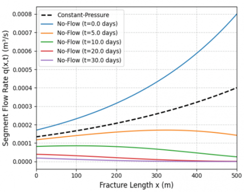
A single curve represents the constant‑pressure boundary condition (black, dashed), while multiple curves show the no‑flow boundary condition at different times.
Figure 5 illustrates the profiles of segment flow rate $q$ under different boundary conditions and production times. Under the constant-pressure condition, the segment flow rate gradually increases toward the wellbore from the fracture tip. For the no-flow boundary, the initial profile at $t=0$ exhibits a similar shape but with a higher magnitude of flow rate. However, as production time progresses under the no-flow boundary, this expected trend no longer holds: reservoir depletion causes the inflow near the wellbore to decline so sharply that, at later times, the segment flow rate close to the wellbore can fall below the flow rate contributed by segments farther from the wellbore. This phenomenon can be explained by Figure 6 that illustrates the pressure profiles along fracture length. Notably, flow rate is a volumetric quantity. To calculate the flow rate at a given location $x$, the fracture length is discretized into 100 segments, each with a segment length of $\Delta x=50 \mathrm{~m}$.
Figure 5. Segment flow rate distribution along the fracture
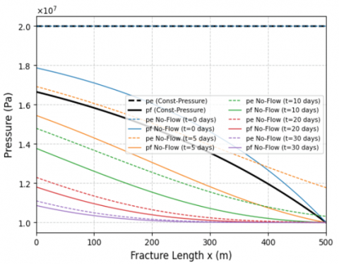
Figure 6. Profiles of $p_e$ and $p_f$ along fracture length for both constant pressure and no-flow boundary conditions
In Figure 6, black solid and dashed lines represent the distribution of $p_e$ and $p_f$ under the constant-pressure boundary condition. Because this assumption imposes a fixed external boundary pressure, $p_e$ remains constant across the entire fracture length, appearing as a horizontal line. In contrast, the fracture pressure $p_f$ declines from the fracture tip toward the wellbore, creating an increasing pressure differential $\left(p_e-p_f\right)$ closer to the wellbore. This growing differential explains why the high segment flow rate near the wellbore under constant-pressure conditions. However, under no-flow boundary conditions, the depletion of $p_e$ is directly linked to the segment flow rate $q$. Higher flow rates accelerate the depletion of $p_e$, which in turn reduces the pressure differential $\left(p_e-p_f\right)$ and negatively impacts subsequent inflow. In Figure 6, $p_e$ and $p_f$ at the same time step are plotted using the same color, with solid lines for $p_f$ and dashed lines for $p_e$ to facilitate comparison. At any given time, a larger gap between $p_e$ and $p_f$ corresponds to a higher segment flow rate at that location. At later times, this gap narrows while approaching the wellbore, which aligns with the segment flow rate evolution shown in Figure 5.
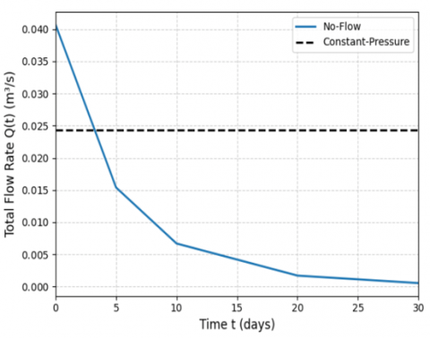
Figure 7 presents cumulative flow rate profiles, calculated as the integral of segment flow rates along the fracture length $x_f$. Under the constant‑pressure boundary condition, the cumulative rate remains constant over time, reflecting the assumption of an unlimited external pressure source. In contrast, for the no‑flow boundary condition, the cumulative rate starts high but declines significantly over time as reservoir pressure depletes, illustrating the nature of fluid flow under closed‑boundary conditions.
Figure 7. Comparison of cumulative flow rate profiles at different times for the no‑flow and constant‑pressure boundary conditions
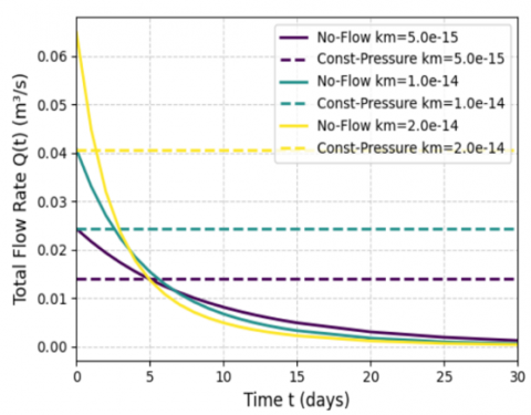
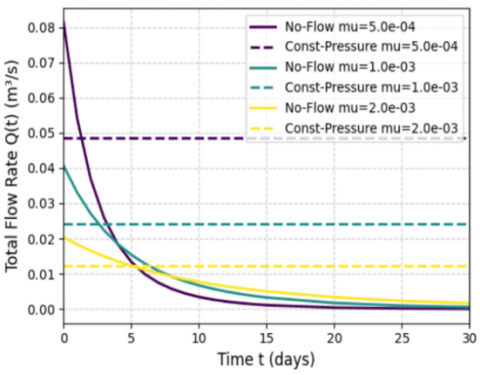
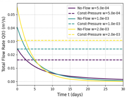
A series of sensitivity tests was carried out to evaluate the influence of matrix permeability ($k_m$), fluid viscosity ($\mu$), and fracture aperture ($w$) on the cumulative flow rate response. Figures 8-10 illustrate how variations in these parameters affect the cumulative flow rate $Q(t)$ under both no-flow and constant-pressure boundary conditions, respectively. In all figures, solid lines represent the no-flow solutions, while dashed lines represent the corresponding constant-pressure solutions.
Figure 8. Sensitivity of cumulative flow rate $Q(t)$ under noflow and constant-pressure boundary conditions to varying matrix permeabilities ( $k_m=5 \times 10^{-15}, 1 \times 10^{-14}, 2 \times \left.10^{-14} \cdot m^2\right)$
Figure 9. Sensitivity of cumulative flow rate $Q(t)$ under no-flow and constant-pressure boundary conditions to varying fluid viscosities $\left(\mu=5 \times 10^{-4}, 1 \times 10^{-3}, 2 \times 10^{-3} \cdot p a \cdot s\right)$
Figure 10. Sensitivity of cumulative flow rate $Q(t)$ under no-flow and constant-pressure boundary conditions to varying fracture aperture widths $\left(w=5 \times 10^{-4}, 1 \times 10^{-3}, 2 \times 10^{-3} \cdot m\right)$
Figure 8 examines the effect of matrix permeability on cumulative flow rate. Higher permeability values produce markedly higher flow rates for both boundary conditions by improving connectivity between the matrix and fracture. Under no-flow conditions, the enhanced permeability results in a strong initial surge in flow that declines rapidly as the system depletes, while the constant-pressure curves remain steady but scale upward with permeability. Figure 9 investigates the impact of fluid viscosity on cumulative flow rate. Lower viscosity promotes significantly higher flow rates by reducing hydraulic resistance. Figure 10 explores the role of fracture aperture on cumulative flow rate. The constant-pressure curves rise in magnitude with aperture, while the no-flow curves reveal sharper early-time surges followed by more rapid depletion for the wider fracture scenarios.
In this work, analytical models of DCF were successfully developed by deriving and solving a differential–integral equation that describes fluid transfer from the shale matrix into hydraulic fractures. By assuming the pseudo-steady-state regime and neglecting horizontal flow in rock matrix, this formulation provides a clear mathematical framework for evaluating fracture–matrix interactions under different boundary conditions. It is important to note that this study is fundamentally theoretical: the “validation” discussed here refers to the mathematical rigor and internal consistency of the solutions, rather than direct comparison with field data. Full-scale validation using field observations, which would involve additional complexities such as reservoir heterogeneity and operational variability, remains outside the present scope. Future work should apply this analytical framework to field data to assess its predictive performance and refine the model for practical deployment. Some conclusions can be drawn as follows:
•The analytical solution offers key advantages over purely numerical methods. It provides explicit expressions for pressure and flow distributions, enabling rapid computation, straightforward sensitivity analysis, and intuitive understanding of the impact of fracture geometry, boundary conditions, and reservoir properties—all without the computational burden of fully discretized models.
•Results from the derived equations clarify the impact of boundary conditions on production. Under a no-flow boundary, cumulative flow rates start higher than those under constant-pressure boundaries due to fluid expansion effects but decline over time as reservoir pressure depletes. Constant-pressure boundaries maintain steady inflow, offering a useful contrast for field interpretation and forecasting.
•The model demonstrates versatility for engineering applications. It can be applied to different shale formations and fracture configurations and serves as a foundation for hybrid workflows, where analytical solutions guide or benchmark more detailed numerical simulations.
Overall, this study demonstrates that carefully constructed analytical models can complement numerical simulations by offering transparent, efficient, and scalable tools for understanding flow mechanisms in hydraulic-fractured shale reservoirs.
The authors express their gratitude to the Energy Institute of Louisiana at the University of Louisiana at Lafayette for supporting the research.
The differential equation is
$\frac{d^2 p_d(x)}{d x^2}=c p_d$ (A.1)
and
$p_d=p_e-p_f(x)$ (A.2)
The boundary conditions are written as follows:
$\left.p_d\right|_{x=x_f}=p_d^*=p_e-p_w$ (A.3)
and
$\left(\frac{d p_e}{d x}\right)_{p_d=0}=0$ (A.4)
Let
$p_d^{\prime}=\frac{d p_d}{d x}$ (A.5)
then
$\frac{d^2 p_d}{d x^2}=\frac{d p_d^{\prime}}{d x}=\frac{d p_d^{\prime}}{d p_d} \cdot \frac{d p_d}{d x}=p_d^{\prime} \frac{d p_d^{\prime}}{d p_d}$ (A.6)
Substituting this equation to Eq. (A.1) gives:
$p_d^{\prime} \frac{d p_d^{\prime}}{d p_d}=c p_d$ (A.7)
which is integrated to get:
$\frac{1}{2}\left(p_d^{\prime}\right)^2=\frac{1}{2} c\left(p_d\right)^2+c_3$ (A.8)
Apply the boundary condition given by Eq. (A.5) gives $c_3=0$. Then Eq. (A.8) is rearranged to yield:
$\frac{d p_d}{d x}=\sqrt{c} p_d$ (A.9)
which is integrated to get:
$\ln \left(p_d\right)=\sqrt{c} x+c_4$ (A.10)
Apply the boundary condition given by Eq. (A.3) gives:
$c_4=\ln \left(p_d^*\right)-\sqrt{c} x_f$ (A.11)
Substituting this equation to Eq. (A.10) yields:
$\ln \left(\frac{p_d}{p_d^*}\right)=\sqrt{c}\left(x-x_f\right)$ (A.12)
which gives:
$p_d=p_d^* e^{\sqrt{c}\left(x-x_f\right)}$ (A.13)
Substituting Eq. (A.4) into Eq. (A.13) results in:
$p_f(x)=p_e-\left(p_e-p_w\right) e^{\sqrt{c}\left(x-x_f\right)}$ (A.14)
[1] Maxwell, S., Cho, D., Norton, M. (2011). Integration of surface seismic and microseismic part 2: Understanding hydraulic fracture variability through geomechanical integration. CSEG Recorder, 36(2): 27-30.
[2] Warpinski, N.R. (2013). Understanding hydraulic fracture growth, effectiveness, and safety through microseismic monitoring. In ISRM International Conference for Effective and Sustainable Hydraulic Fracturing, Brisbane, Australia, pp. ISRM-ICHF-2013-047.
[3] Abdulaziz, A.M. (2013). Microseismic imaging of hydraulically induced-fractures in gas reservoirs: A case study in Barnett shale gas reservoir, Texas, USA. Open Journal of Geology, 3(5): 361-369.
[4] Barati, R., Liang, J.T. (2014). A review of fracturing fluid systems used for hydraulic fracturing of oil and gas wells. Journal of Applied Polymer Science, 131(16): 40735. https://doi.org/10.1002/app.40735
[5] Li, S., Zhang, D. (2018). A fully coupled model for hydraulic-fracture growth during multiwell-fracturing treatments: Enhancing fracture complexity. SPE Production & Operations, 33(2): 235-250. https://doi.org/10.2118/182674-PA
[6] Feng, F., Wang, X., Guo, B., Ai, C. (2017). Mathematical model of fracture complexity indicator in multistage hydraulic fracturing. Journal of Natural Gas Science and Engineering, 38: 39-49. https://doi.org/10.1016/j.jngse.2016.12.012
[7] Zhang, D., Dai, Y., Ma, X., Zhang, L., Zhong, B., Wu, J., Tao, Z. (2018). An analysis for the influences of fracture network system on multi-stage fractured horizontal well productivity in shale gas reservoirs. Energies, 11(2): 414. https://doi.org/10.3390/en11020414
[8] Wang, J., Ge, H., Wang, X., Shen, Y., Liu, T., Zhang, Y., Meng, F. (2019). Effect of clay and organic matter content on the shear slip properties of shale. Journal of Geophysical Research: Solid Earth, 124(9): 9505-9525. https://doi.org/10.1029/2018JB016830
[9] Xue, L., Dai, C., Wang, L., Chen, X. (2019). Analysis of thermal stimulation to enhance shale gas recovery through a novel conceptual model. Geofluids, 2019(1): 4084356. https://doi.org/10.1155/2019/4084356
[10] Yu, L., Wang, J., Wang, C., Chen, D. (2019). Enhanced tight oil recovery by volume fracturing in Chang 7 reservoir: Experimental study and field practice. Energies, 12(12): 2419. https://doi.org/10.3390/en12122419
[11] Guo, B., Shaibu, R., Hou, X. (2020). Crack propagation hypothesis and a model to calculate the optimum water-soaking period in shale gas/oil wells for maximizing well productivity. SPE Drilling & Completion, 35(4): 655-667. https://doi.org/10.2118/201203-PA
[12] Fu, C., Guo, B., Mokhtari, A. (2021). Quantitative analysis of the sequential initiation and simultaneous propagation of multiple fractures in shale gas/oil formations. Journal of Petroleum Science and Engineering, 200: 108272. https://doi.org/10.1016/j.petrol.2020.108272
[13] Warren, J.E., Root, P.J. (1963). The behavior of naturally fractured reservoirs. Society of Petroleum Engineers Journal, 3(3): 245-255. https://doi.org/10.2118/426-PA
[14] Cinco-Ley, H., Samaniego-V, F. (1981). Transient pressure analysis for fractured wells. Journal of Petroleum Technology, 33(0): 1749-1766. https://doi.org/10.2118/7490-PA
[15] Gringarten, A.C., Ramey Jr, H.J., Raghavan, R. (1974). Unsteady-state pressure distributions created by a well with a single infinite-conductivity vertical fracture. Society of Petroleum Engineers Journal, 14(4): 347-360. https://doi.org/10.2118/4051-PA
[16] Olson, J.E. (2007). Fracture aperture, length and pattern geometry development under biaxial loading: A numerical study with applications to natural, cross-jointed systems. Geological Society London Special Publications, 289(1): 123-142. https://doi.org/10.1144/SP289.8
[17] Han, D., Kwon, S. (2021). Application of machine learning method of data-driven deep learning model to predict well production rate in the shale gas reservoirs. Energies, 14(12): 3629. https://doi.org/10.3390/en14123629
[18] Zhou, W., Li, X., Qi, Z., Zhao, H., Yi, J. (2024). A shale gas production prediction model based on masked convolutional neural network. Applied Energy, 353, 122092. https://doi.org/10.1016/j.apenergy.2023.122092
[19] Hyman, J.D., Jiménez-Martínez, J., Viswanathan, H.S., Carey, J.W., et al. (2016). Understanding hydraulic fracturing: A multi-scale problem. Philosophical Transactions of the Royal Society A: Mathematical, Physical and Engineering Sciences, 374(2078): 20150426. https://doi.org/10.1098/rsta.2015.0426
[20] Dai, S., Chen, C., Wang, H., Fu, Z., Liu, D. (2019). A semianalytical approach for production of oil from bottom water drive tight oil reservoirs with complex hydraulic fractures. Journal of Chemistry, 2019(1): 5186831. https://doi.org/10.1155/2019/5186831
[21] Hu, B., Wang, J., Ma, Z. (2020). A fractal discrete fracture network based model for gas production from fractured shale reservoirs. Energies, 13(7): 1857. https://doi.org/10.3390/en13071857
[22] Huisman, I.H. (2000). Membrane separations| microfiltration. In Encyclopedia of Separation Science, pp. 1764-1777. https://doi.org/10.1016/B0-12-226770-2/05251-0
[23] Ferreira, A.S., Massarani, G. (2005). Physico-mathematical modeling of crossflow filtration. Chemical Engineering Journal, 111(2-3): 199-204. https://doi.org/10.1016/j.cej.2005.02.002
[24] Hakami, M.W., Alkhudhiri, A., Al-Batty, S., Zacharof, M.P., Maddy, J., Hilal, N. (2020). Ceramic microfiltration membranes in wastewater treatment: Filtration behavior, fouling and prevention. Membranes, 10(9): 248. https://doi.org/10.3390/membranes10090248
[25] Mkpuma, V.O., Moheimani, N.R., Ennaceri, H. (2022). Microalgal dewatering with focus on filtration and antifouling strategies: A review. Algal Research, 61: 102588. https://doi.org/10.1016/j.algal.2021.102588
[26] Kazemi, M.A., Soltanieh, M., Yazdanshenas, M. (2013). Mathematical modeling of crossflow microfiltration of diluted malt extract suspension by tubular ceramic membranes. Journal of Food Engineering, 116(4): 926-933. https://doi.org/10.1016/j.jfoodeng.2013.01.029
[27] Park, G.W., Nägele, G. (2020). Modeling cross-flow ultrafiltration of permeable particle dispersions. The Journal of Chemical Physics, 153(20): 204110. https://doi.org/10.1063/5.0020986
[28] Parasyris, A., Discacciati, M., Das, D.B. (2020). Mathematical and numerical modelling of a circular cross-flow filtration module. Applied Mathematical Modelling, 80: 84-98. https://doi.org/10.1016/j.apm.2019.11.016
[29] Bradley, J.C. (2010). Counterflow, crossflow and cocurrent flow heat transfer in heat exchangers: Analytical solution based on transfer units. Heat and Mass Transfer, 46(4): 381-394. https://doi.org/10.1007/s00231-010-0579-5
[30] Liu, Y., Li, K., Wen, J., Wang, S. (2023). Thermodynamic characteristics of counter flow and cross flow plate fin heat exchanger based on distributed parameter model. Applied Thermal Engineering, 219: 119542. https://doi.org/10.1016/j.applthermaleng.2022.119542