Jamil Safarov![]() | Ramil I. Hasanov*
| Ramil I. Hasanov*![]() | Emiliya Huseynova
| Emiliya Huseynova![]() | Arzu Safarli
| Arzu Safarli![]()
© 2025 The authors. This article is published by IIETA and is licensed under the CC BY 4.0 license (http://creativecommons.org/licenses/by/4.0/).
OPEN ACCESS
Aluminum serves as a cornerstone in promoting environmentally sustainable practices, underscoring the strategic importance of the global aluminum industry within the framework of the evolving green economy. Primary aluminum production (PAP) has experienced a significant upward trend over the past five decades, reflecting the growing demand across various industrial sectors worldwide. This study advances production forecasting methodologies by integrating time series analysis, incorporating a range of scenarios from a central baseline to optimistic and pessimistic perspectives. Through the utilization of the AutoRegressive Integrated Moving Average (ARIMA) model, the research offers forecasts of PAP trends until 2030, conducting a comprehensive analysis of the industry's trajectory. Through empirical examination, the forecast reveals a consistent upward trajectory in global PAP. Volumes are anticipated to increase from around 70 million tonnes in 2023 to more than 82 million tonnes by 2030, representing an overall growth of approximately 17%. The model selection and validation procedures involved stationarity testing, analysis of autocorrelation patterns, and evaluation using information criteria to ensure robustness and reliability. Forecasts are presented with confidence intervals to account for uncertainty in future production estimates. This anticipated expansion highlights the enduring global demand and the critical role of aluminum in supporting industrial development and the green energy transition.
primary aluminum production (PAP), AutoRegressive Integrated Moving Average (ARIMA) model, statistics, time series forecasting, mathematical modelling
The growing demand for aluminum, often called the metal of the future, stems from its unique physical properties, durability, and eco-friendly attributes. Consequently, global aluminum production continues to rise, nearing levels historically dominated by iron, the traditional foundation of the metallurgical industry.
Primary aluminum refers to aluminum extracted from electrolytic cells or pots during the electrolytic reduction process of metallurgical aluminum oxide. The method known as the Hall-Héroult process, discovered independently in 1886 by Charles Martin Hall from the United States and Paul Héroult from France, remains the principal industrial process for producing primary aluminum [1]. The various chemical, electrochemical, and thermal processes involved in aluminum production from alumina are thoroughly examined, encompassing activities such as refining alumina, conducting electrolysis, and implementing recycling techniques [2].
From 2000 to 2020, worldwide aluminum production more than doubled. China played a pivotal role in this growth, accounting for 57 percent of global aluminum production in 2020 [3]. In 2023, China accounted for 41.5 million tons of primary aluminum production (PAP) out of the world's total production of 70 million tons [4]. Azerbaijan stands as the sole primary aluminum producer in the Caucasus region. The Ganja Aluminum Complex, operational for over a decade, spearheads this endeavor. With an annual PAP volume ranging between 50,000 to 55,000 tons, the complex is poised to double its output in the foreseeable future [5]. Investigating and forecasting future trends within the aluminum industry, which holds significant promise for economic development, is crucial both on a global scale and within local contexts. Although prior research has predominantly concentrated on regional output and aluminum pricing frameworks, there is a notable scarcity of studies offering long-term, data-driven forecasts of global PAP based on rigorous statistical techniques. Furthermore, the incorporation of scenario-based modeling to evaluate alternative future pathways remains underexplored. This study seeks to bridge this gap by utilizing the AutoRegressive Integrated Moving Average (ARIMA) time series forecasting approach to project global aluminum production trends through 2030 under baseline.
The primary aluminum industry is associated with substantial carbon emissions, presenting a pressing concern due to its role as a primary contributor to global climate change, especially in tandem with increased production. The focal point of both the global business and scientific spheres is the imperative to reduce CO2 emissions while concurrently expanding production within this industry, leading to numerous scholarly inquiries into this matter [6]. Subsequent phases of aluminum production primarily involve chemical processing operations, characterized by significantly reduced levels of carbon emissions [7].
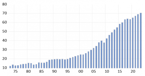
Figure 1 illustrates the global PAP spanning the last five decades, indicating a predominant trend towards growth. Notably, even during the periods of the 2007-2008 financial crisis and the 2020-2021 COVID-19 pandemic, which significantly impacted numerous industries, the primary aluminum sector remained resilient, experiencing swift recoveries following each crisis.
A time series refers to an organized collection of data points systematically recorded at uniform intervals over time. These data points encapsulate a wide array of variables, including sales, temperature variations, stock prices, and production quantities. The primary objective of time series forecasting is to anticipate upcoming values by drawing upon insights gleaned from past observations and patterns. Such forecasting efforts aim to provide predictive insights into future trends and behaviors within the examined field. Before embarking on the forecasting process, it is essential to undertake a thorough examination of statistical data and diagnostic assessments covering multiple decades. This preliminary step provides a foundational understanding of historical trends and patterns, facilitating informed decision-making during the forecasting endeavor.
Forecasting PAP using mathematical models is essential for efficient resource management, cost reduction, and meeting market demand. Advanced forecasting enables producers to optimize capacity planning, raw material procurement, and inventory management, thereby improving operational efficiency and competitiveness. The novelty of this research lies in its global approach to forecasting, the use of long-term historical data (1973–2023), and the application of the ARIMA model within a scenario-based framework. The study contributes to the academic literature by offering a robust and interpretable statistical model for long-term production forecasting. Practically, the findings provide policymakers, manufacturers, and supply chain planners with vital projections to support informed decision-making in the context of resource management, market planning, and the broader green transition.
Various mathematical methods and models are employed to forecast future trends based on historical patterns. The ARIMA model, first introduced by Box and Jenkins [8], serves as a cornerstone in time series forecasting. The ARIMA model adeptly captures temporal trends and patterns by examining the impact of previous observations through autoregressive examination, rectifying data stationarity via integration, and accommodating stochastic fluctuations via a moving average technique. This adaptable framework has firmly entrenched ARIMA as a favored methodology for forecasting across a diverse array of fields encompassing finance, business, and engineering disciplines. Additionally, it has been employed in analyses involving consumption, imports, and exports.
In their study, Kriechbaumer et al. [9] presented a new technique that integrate wavelet analysis with ARIMA models to enhance the predictive accuracy of cyclical metal prices, including those of aluminum, copper, lead, and zinc. Kalantzis [10] examined the feasibility of leveraging past data on aluminum producers' stocks, economic indices, currency values, and other commodity prices to statistically forecast future aluminum prices. The aim is to construct a reliable price forecasting model for this essential metal. Several research studies have also investigated the forecasting of aluminum production. Khalil and Hamad [11] examined the effectiveness of ARIMA and ANN models in forecasting monthly aluminum exports from Turkey to Iraq. Their analysis reveals that ANN outperforms ARIMA, as evidenced by lower error metrics, indicating its superior accuracy for this forecasting task. ARIMA is a widely used, interpretable method suitable for long-term forecasting with stable historical patterns, though its linear nature may limit performance with complex data. In contrast, ANN and hybrid models handle nonlinearities better but require larger datasets, more computation, and offer less transparency. The choice between ARIMA and ANN depends on data availability, forecasting goals, and the trade-off between accuracy and interpretability.
In his study, Sas [12] investigated the potential effects of variables such as GDP, population size, and the expansion of key industries on the future trajectory of aluminum production in India for the next twenty years. Furthermore, a variety of other econometric forecasting and diagnostic articles have been developed [13-15]. The provided scientific samples offer both theoretical insights and practical information concerning existing research. Although ARIMA offers transparency and simplicity, it may fall short in capturing volatility and nonlinear trends. Recent models like LSTM [16] and Prophet [17] better handle such complexities, while integrated approaches combining econometric and technical factors are gaining prominence in production forecasting. This study uses ARIMA as a baseline, with recognition of these advanced alternatives.
The initial step in our analysis involves describing the dataset for PAP. This dataset, covering the period from 1973 to 2023, was obtained from the International Aluminum Institution [18] and comprises annual production figures, forming the foundation for our forecasting model. Before delving into time series modeling, it is essential to ascertain the stationarity of the PAP data. This entails conducting a unit root test, such as the Augmented Dickey-Fuller test, to discern any underlying trends or seasonality within the dataset. In cases where the data exhibits non-stationarity, differencing techniques may be applied to render it stationary. Subsequently, we analyze the autocorrelation function (ACF) and partial autocorrelation function (PACF) of the PAP data. These analyses aid in identifying potential autoregressive (AR) and moving average (MA) terms suitable for inclusion in our ARIMA model. The ACF plot illustrates the correlation between the current observation and its lagged values, while the PACF plot reveals the direct relationship between the current observation and its lagged values after accounting for intermediate lag effects. Based on diagnostic results, we select the most appropriate ARIMA model for forecasting global PAP, which entails specifying values for the autoregressive (p), differencing (d), and moving average (q) terms.
The ARIMA model, a commonly utilized tool in time series analysis, can be succinctly expressed as follows [19]:
Yₜ = c + φ₁Yₜ₋₁ + φ₂Yₜ₋₂ + ... + φₚYₜ₋ₚ + θ₁eₜ₋₁ + θ₂eₜ₋₂ + ... + θₑ₋₁ + θₑ₋₂ + ... + θ_qeₜ₋_q + eₜ (1)
In this equation, Yₜ represents the PAP at time t, while c denotes a constant term. The parameters ϕ₁, ϕ₂, ..., ϕₚ denote the autoregressive elements, signifying the influence of previous PAP values on the current value. Similarly, θ₁, θ₂, ..., θq symbolize the moving average parameters, depicting the impact of prior forecast errors on the present value. The term eₜ indicates the error term at time t, crucial for capturing unexplained variability in the data. The variables p and q signify the order of the autoregressive and moving average components, respectively, offering valuable insights into temporal dependencies within the dataset.
Applying first differencing (d=1) successfully eliminated non-stationarity in the series, while analysis of the autocorrelation and partial autocorrelation functions identified one significant autoregressive term (p=1) and one moving average term (q=1). This specification also yielded the lowest values of information criteria (Akaike Information Criterion (AIC) and Bayesian Information Criterion (BIC)) relative to alternative models, suggesting an optimal balance between model fit and parsimony.
Table 1 presents data on PAP, indicating the quantity of aluminum produced directly from electrolytic cells during the reduction of aluminum oxide. Notably, this metric excludes any alloying additives or recycled aluminum, focusing solely on the primary production process.
The dataset spanning from 1973 to 2023 demonstrates an average production of roughly 31,360 thousand metric tonnes and a median production level of approximately 22,721 thousand metric tonnes. A positive skewness value of 0.843 indicates years characterized by notably high production levels, while a kurtosis value of 2.229 suggests a distribution with a relatively flat peak.
Table 1. Data description of APA in level
|
Mean |
Median |
Max |
Min |
Std. Dev. |
Skewness |
Kurtosis |
|
31.360 |
22.721 |
70.581 |
12.017 |
18.926 |
0.843 |
2.229 |
Evaluating stationarity stands as a pivotal element within econometric inquiry, as it forms the cornerstone for the fundamental assumptions and methodologies utilized in empirical investigations within the field of economics. The Augmented Dickey-Fuller (ADF) test is an indispensable statistical tool for analyzing the stationarity of time series data. Mushtaq [20] explores the significance of examining data for stationarity, particularly emphasizing the temporal aspects of underlying variables. Although not explicitly mentioning the Augmented Dickey-Fuller (ADF) test, the abstract highlights the crucial role of conducting stationarity tests in academic research.
Table 2 demonstrates that the initial assessment indicates a lack of stationarity in the time series, with p-values exceeding 0.05 in both instances. Nevertheless, after employing first differencing, the time series achieves stationarity, evidenced by significantly reduced p-values. This suggests that differencing effectively eliminates the inherent trend, enabling the time series to undergo stationary analysis.
Table 2. ADF unit root test
|
Deterministic Components |
Test Statistics |
Level |
1st Difference |
|
Intercept |
p-value |
1.0000 |
0.0002 |
|
t-statistic |
3.225916 |
-4.949230 |
|
|
Trend and Intercept |
p-value |
0.9595 |
0.0000 |
|
t-statistic |
0.791352 |
-6.356726 |
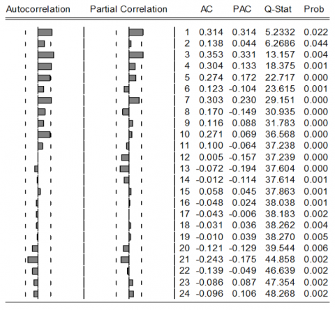
Figure 2 displays the correlogram output, a diagnostic tool used to evaluate autocorrelation within the residuals of an ARIMA model, reflecting the serial dependence of errors in a time series model. The correlogram showcases the ACF and PACF of the residuals, quantifying the correlation between residuals at different lags. Interpretation entails examining autocorrelation (AC) and partial autocorrelation (PAC) coefficients, as well as the Ljung-Box Q statistic and its corresponding p-values, with significant deviations suggesting notable autocorrelation, potentially indicating model inadequacies necessitating adjustments like the inclusion of additional AR or MA terms.
Figure 2. Correlogram of PAP. The analysis was conducted utilizing the EViews software platform
The main criteria from the diagnostics selects that the most appropriate model for analyzing time series data is ARMA (1,1,1). We perform estimation for the following equation to identify a potential candidate model for forecasting, ultimately leading to the forecast:
∆PAPₜ = c + φ₁PAPₜ₋₁ + θ₁εₜ₋₁ + εₜ (2)
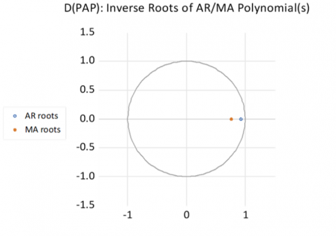
When evaluating the stability of a univariate process, it is essential to verify that the model residuals exhibit characteristics consistent with White Noise, a fundamental requirement for model integrity. This assessment typically involves employing statistical tests like the Ljung-Box Q statistic to examine the null hypothesis concerning the absence of autocorrelation in the residuals. Within this framework, the stability of the estimated Autoregressive Moving Average (ARMA) model critically depends on the positioning of its roots within the unit circle: AR roots residing within this circle denote covariance and stationarity, while MA roots within the circle ensure the invertibility of the ARMA process. In the realm of time series analysis, AR and MA models are frequently utilized for data modeling, wherein the properties of the model are dictated by the reciprocal roots of these polynomials, highlighting their crucial role in elucidating the temporal dynamics of the dataset. ARMA is a common method for time series forecasting. In Figure 3, the horizontal axis of the plot is annotated as "AR roots" and "MA roots". This plot constructs a model by incorporating historical data points from a time series while also accounting for the stochastic nature of the error terms.
Figure 3. D(PAP): Inverse roots of AR (1) MA (1) Polynomial (s)
The AR and MA parts of the ARMA model refer to two types of polynomials used in the model. AR stands for autoregressive, and it refers to how past values of the time series affect future values. MA stands for moving average, and it refers to how the randomness of the error terms affects future values. The positioning of the roots of the ARMA polynomials can impact both the stability and forecasting capabilities of the model.
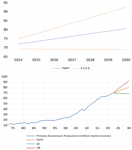
While the ARIMA model is primarily utilized in forecasting analyses within the financial domain, there exist notable scholarly investigations concerning production forecasting as well [21-24]. Figure 4 illustrates the historical and projected trend lines for global PAP spanning from 2023 to 2030. The vertical axis denotes production quantity, while the horizontal axis signifies the years. The central forecast line (PAPF) acts as the baseline forecasting, drawing upon historical data and an ARIMA model, while the upper bound (UB) and lower bound (LB) delineate optimistic and pessimistic scenarios, respectively.
Figure 4. Forecasting global PAP trends: 2023-2030
Notably, historical data indicates a consistent upward trend in PAP over time. Moving forward, the forecast suggests a continuation of this growth trajectory. Optimistically, favorable conditions such as technological advancements and increased demand could propel production levels beyond the central forecast, while challenges like sup-ply chain disruptions or economic downturns may result in production falling below expectations.
The ARIMA model integrates a resilient algorithm for time series forecasting, incorporating AR, differencing (I), and MA elements. Fundamentally, the model utilizes historical data points from the time series to project forthcoming values, based on the premise that knowledge derived from prior observations can aptly guide forecasts of future trends. The aluminum industry exhibits dynamic characteristics and operates within an evolving business environment within the global economy. According to the FBI [25], the global aluminum market reached a valuation of \$\262.75 billion in 2022. Projections suggest further growth, with the market expected to reach \$229.85 billion in 2023 and a significant increase to approximately \$393.70 billion by 2032. Mathematical modeling facilitates forecast analysis based on historical data, yet it does not guarantee complete accuracy in forecasting future outcomes. Numerous factors influencing economic forecasts can significantly diminish the precision of mathematical observations. For instance, global economic downturns can drastically reduce demand and production levels. Conversely, upward trends in the global economy may necessitate higher production volumes. Moreover, the increasing recognition of aluminum as an environmentally friendly metal could lead to a substantial surge in demand in the future. Forecasts suggest that by 2030, demand for aluminum, driven by sectors like transportation and construction, could surge by as much as 40%, surpassing the forecasts generated by mathematical models [26]. Indeed, there exist distinctions between econometric mathematical forecasting and demand forecasts. Nonetheless, the narrative outcomes of both avenues indicate a consensus: aluminum production is poised to escalate in the future, underscoring the growing significance of this strategic industry.
The optimistic and pessimistic scenarios function as simplified, qualitative frameworks intended to encompass a spectrum of potential future developments. The optimistic scenario envisions favorable factors such as sustained economic expansion and enabling policy environments that promote higher aluminum production. Conversely, the pessimistic scenario accounts for limiting factors including reduced economic growth, tighter regulatory measures, or disruptions in supply chains. While these scenarios are not elaborated with quantitative detail in the present analysis, they offer important contextual insights into possible production pathways and lay the groundwork for more detailed, quantitative modeling in subsequent research.
The rising trend in global PAP is influenced by factors including technological progress, market demand, energy supply, and geopolitical dynamics. This study utilized time series analysis to assess production patterns from 1973 to 2023, identifying a positively skewed distribution and non-stationary behavior, which were effectively captured through an ARIMA (1,1,1) model. The projections suggest a sustained increase in primary aluminum output across different scenarios, highlighting the sector’s expanding strategic significance.
Key findings emphasize the appropriateness of ARIMA for production forecasting and acknowledge the inherent volatility in historical production data. Nonetheless, the study is limited by the omission of explicit external determinants such as environmental regulations, economic policy changes, and potential disruptive technological innovations that could influence future production trajectories. Subsequent research should aim to incorporate these quantitative drivers to enable more robust scenario-based forecasting. Moreover, factoring in emission reduction targets and sustainability objectives will be crucial to ensure alignment of production forecasts with global climate commitments.
[1] The Aluminum Association. (2021). Primary Production 101. https://www.aluminum.org/primary-production-101.
[2] Tabereaux, A.T., Peterson, R.D. (2014). Aluminum production. Treatise on Process Metallurgy, 3: 839-917. https://doi.org/10.1016/B978-0-08-096988-6.00023-7
[3] Global Efficiency Intelligence. (2023). Aluminum Industry. https://www.globalefficiencyintel.com/aluminum-industry.
[4] Sengupta, D. (2024). China’s 2023 primary aluminium production establishes a new high recording an 11% annual rise. https://www.alcircle.com/news/chinas-2023-primary-aluminium-production-establishes-a-new-high-recording-an-11-annual-rise-105685#:~:text=According%20to%20the%20Shanghai%20Metals,tonnes%20in%20the%20entire%20year.
[5] Hasanov, R.I. (2023). The role of the aluminum industry in Azerbaijan's economy: A general overview. Business & IT, XIII(1): 48-57. https://doi.org/10.14311/bit.2023.01.06
[6] Hasanov, R., Safarov, J., Safarli, A. (2024). Analyzing and forecasting CO2 emissions in the aluminum sector using ARIMA model. Agora International Journal of Economical Sciences, 18(1): 55-64. https://doi.org/10.15837/aijes.v18i1.6710
[7] Tabereaux, A.T., Peterson, R.D. (2024). Aluminum production. Treatise on Process Metallurgy, 3: 625-676. https://doi.org/10.1016/B978-0-323-85373-6.00004-1
[8] Box, G., Jenkins, G.M. (1976). Time Series Analysis: Forecasting and Control. Holden Day, San Francisco.
[9] Kriechbaumer, T., Angus, A., Parsons, D., Casado, M.R. (2014). An improved wavelet–ARIMA approach for forecasting metal prices. Resources Policy, 39: 32-41. https://doi.org/10.1016/j.resourpol.2013.10.005
[10] Kalantzis, C. (2020). Aluminium Price prediction models using data analysis. MSc thesis. https://apothesis.eap.gr/archive/item/151377.
[11] Khalil, D.M., Hamad, S.R. (2023). A comparison of artificial neural network models and time series models for forecasting Turkey's monthly aluminium exports to Iraq. Journal of Survey in Fisheries Sciences, 10(1S): 4262-4279.
[12] Sas, S.S. (2012). Future of aluminium industry in India Doctoral Dissertation. National Institute of Technology Rourkela. http://ethesis.nitrkl.ac.in/3602/.
[13] Gilbert, C.L. (1995). Modelling market fundamentals: A model of the aluminium market. Journal of Applied Econometrics, 10(4): 385-410. https://doi.org/10.1002/jae.3950100405
[14] Dooley, G., Lenihan, H. (2005). An assessment of time series methods in metal price forecasting. Resources Policy, 30(3): 208-217. https://doi.org/10.1016/j.resourpol.2005.08.007
[15] Hutami, A., Ajidarma, P., Irianto, D. (2022). Cost minimization model for raw materials procurement planning at an Indonesian aluminium producer. In Proceedings of the International Manufacturing Engineering Conference & The Asia Pacific Conference on Manufacturing Systems, pp. 517-526. https://doi.org/10.1007/978-981-99-1245-2_48
[16] Flunkert, V., Salinas, D., Gasthaus, J. (2020). DeepAR: Probabilistic forecasting with autoregressive recurrent networks. International Journal of Forecasting, 36(3): 1181-1191. https://doi.org/10.1016/j.ijforecast.2019.07.001
[17] Taylor, S.J., Letham, B. (2018). Forecasting at scale. The American Statistician, 72(1): 37-45. https://doi.org/10.1080/00031305.2017.1380080
[18] International Aluminium (2024). Primary aluminium production. https://international-aluminium.org/statistics/primary-aluminium-production/.
[19] Box, G.E.P., Jenkins, G.M., Reinsel, G.C. (2008). Time Series Analysis: Forecasting and control. John Wiley & Sons.
[20] Mushtaq, R. (2011). Augmented dickey fuller test. https://ssrn.com/abstract=1911068.
[21] Fan, D., Sun, H., Yao, J., Zhang, K., Yan, X., Sun, Z. (2021). Well production forecasting based on ARIMA-LSTM model considering manual operations. Energy, 220: 119708. https://doi.org/10.1016/j.energy.2020.119708
[22] Kumar, M., Anand, M. (2014). An application of time series ARIMA forecasting model for predicting sugarcane production in India. Studies in Business and Economics, 9(1): 81-94.
[23] Badmus, M.A., Ariyo, O.S. (2011). Forecasting cultivated areas and production of maize in Nigerian using ARIMA Model. Asian Journal of Agricultural Sciences, 3(3): 171-176.
[24] Iqbal, N., Bakhsh, K., Maqbool, A., Ahmad, A.S. (2005). Use of the ARIMA model for forecasting wheat area and production in Pakistan. Journal of Agriculture and Social Sciences, 1(2): 120-122.
[25] Aleksić, J., Vargas, D.B. (2024). Aluminium demand will rise 40% by 2030. Here’s how to make it sustainable. In World Economic Forum. https://www.weforum.org/agenda/2023/11/aluminium-demand-how-to-make-it-sustainable/.
[26] Fortune Business Insights. (2024). Metals & Minerals. Aluminium Market. The global aluminium market size was valued at \$262.75 billion in 2022 & is projected to grow from \$229.85 billion in 2023 to \$393.70 billion by 2032. https://www.fortunebusinessinsights.com/industry-reports/aluminium-market-100233.