Alfi Amalia*![]() | Isra Hayati
| Isra Hayati![]() | Ahmad Afandi
| Ahmad Afandi![]() | Andrew Satria Lubis
| Andrew Satria Lubis![]() | Jonathan Liviera Marpaung
| Jonathan Liviera Marpaung![]()
© 2025 The authors. This article is published by IIETA and is licensed under the CC BY 4.0 license (http://creativecommons.org/licenses/by/4.0/).
OPEN ACCESS
This study aims to compare the forecasting performance of Autoregressive Integrated Moving Average (ARIMA) and Support Vector Regression (SVR) models in predicting the monthly stock prices of PT. Telkom Indonesia (TLKM), one of Indonesia's leading state-owned enterprises. Utilizing historical data from January 2018 to December 2022, the models are evaluated based on their forecasting precision using Mean Absolute Percentage Error (MAPE) and Root Mean Square Error (RMSE) as investor-grade performance metrics. The ARIMA (2,1,2) model was selected through Box–Jenkins methodology, while the SVR was optimized using a linear kernel and tuned hyperparameters. The results demonstrate that ARIMA outperforms SVR in both MAPE (2.01%) and RMSE (64.38), indicating better adaptability to the structured linear patterns found in the stock price series. Assumption-based forecasting simulations, extended to the year 2026, further suggest ARIMA’s relative stability, although future projections remain subject to structural and market uncertainties. The findings emphasize the continued relevance of classical statistical models in investment-grade forecasting, where investor-grade is defined as forecasting precision achieving MAPE values below 5%, supporting decision-support applications in emerging markets.
Autoregressive Integrated Moving Average (ARIMA), Support Vector Regression (SVR), financial forecasting, stock price prediction, time series analysis, emerging markets
The increasing volatility of financial markets, especially in emerging economies, presents a major challenge for investors, policymakers, and analysts alike. Fluctuations in stock prices can be abrupt and nonlinear, driven by macroeconomic shocks, political uncertainty, and investor sentiment. For instance, during the COVID-19 pandemic, the Jakarta Composite Index (JCI) experienced a decline of over 37% in Q1 2020, followed by a sharp rebound of 30% within just two months illustrating the unstable dynamics of Indonesian capital markets.
This level of volatility necessitates the development of robust forecasting models that go beyond descriptive analytics. Investor-grade forecasting precision becomes crucial for minimizing exposure to financial risk, timing market entry and exit points, and optimizing asset allocation strategies. In engineering terms, the stock market can be modeled as a nonlinear, stochastic system where signal extraction (i.e., identifying true trends amid noise) is critical for system performance in this case, investment return.
Traditional forecasting approaches often fail to provide the level of predictive stability needed for real-time decision support. Therefore, advanced statistical learning models such as Autoregressive Integrated Moving Average (ARIMA) and Support Vector Regression (SVR) are increasingly applied to model financial time series. These models, when calibrated correctly, can serve as computational engines for algorithmic trading platforms and portfolio optimization tools in volatile and resource-constrained market environments.
Despite the growing importance of data-driven investment strategies, conventional forecasting models such as simple moving averages, exponential smoothing, or even linear regression often fall short when applied to the intricate dynamics of financial markets. These models typically assume stationarity, linearity, and time-invariant relationships, which rarely hold true in real-world stock price movements especially in emerging markets where structural breaks, volatility clustering, and nonlinearity are prevalent.
For instance, in the case of PT. Telkom Indonesia (TLKM), stock prices between 2020 and 2022 fluctuated within a wide band of IDR 2,600 to IDR 4,400, driven by pandemic-induced shocks, digital infrastructure investments, and shifting investor sentiment. Capturing such variation requires forecasting models that not only learn from past patterns but can also adapt to new regimes or anomalies in market behavior.
Moreover, traditional time series models lack the precision and real-time responsiveness expected in today’s algorithmic finance applications. Investors require models capable of providing investor-grade forecasting precision, enabling more reliable entry-exit timing, portfolio hedging, and risk-adjusted return optimization. Thus, there is a pressing need to evaluate and compare advanced statistical learning approaches such as ARIMA and SVR that can provide more nuanced, scalable, and accurate forecasts tailored for investor-centric decision-making in volatile equity environments.
While numerous studies have explored the application of ARIMA and SVR models in stock price forecasting, a focused comparative analysis tailored to the Indonesian equity market remains scarce. as shown by Akhter et al. [1] applied nonlinear autoregressive distributed lag (NARDL) and machine learning algorithms to forecast Bangladesh’s export performance, highlighting structural dependencies in macroeconomic indicators. In energy forecasting, Al-Duais and Al-Sharpi [2] proposed a Markov Chain Monte Carlo time series model for wind power prediction, demonstrating robustness in uncertain conditions. Al-Rousan et al. [3] examined the geopolitical and economic impact of the Russo-Ukrainian war, oil prices, and COVID-19 on global food security, emphasizing the role of external shocks in forecast volatility. In the financial sector, AlMadany et al. [4] compared classical statistical and deep learning models for cryptocurrency return prediction, while Banaś and Utnik-Banaś [5] evaluated SARIMA models with exogenous variables for short-term timber price forecasting. Di Mauro et al. [6] introduced a hybrid learning strategy for forecasting Recent studies have applied hybrid models to improve forecasting accuracy. Ensafi et al. [7] conducted a comparative analysis of machine learning models for seasonal sales forecasting, and Falatouri et al. [8] compared SARIMA and LSTM in retail demand forecasting, concluding that model selection is highly context-dependent. Similarly, ARIMA-SVR combinations, ARIMA-ANN, and ensemble AI models for financial markets [9]. Gong and Lin [10] proposed dummy variable integration to improve volatility forecasting in the electricity sector. Other sector-specific studies include Gong and Lin [10], who applied time series modeling to forecast LNG shipbuilding demand. Lee and Xia [11] used deep learning to analyze the maturity dynamics of crude oil spot and futures prices. Similarly, Maya Sari and Ak [12], and Zulia Hanum [13] studied stock prices using traditional metrics but did not utilize SVR or compare it with ARIMA. No study to date has directly compared ARIMA and SVR as standalone models on Indonesian stock price data, which this paper addresses. Their findings indicated that the hybrid model outperformed individual ARIMA and SVR models. Nevertheless, their study primarily focused on the hybrid approach without a detailed comparative analysis of standalone ARIMA and SVR models. Liu et al. [14], who evaluated tourism recovery post-COVID-19 using time-varying models. Polestico et al. [15] demonstrated improvements through hybrid models such as ARIMA–SVR, ARIMA–ANN, and ensemble AI, although these often obscure the standalone strengths of ARIMA and SVR. Qureshi et al. [16] applied AI techniques to forecast real exchange rates, validating the adaptability of hybrid models. Seasonal and structural components have also been investigated. From a local perspective, financial modeling in Indonesia includes studies on cash holdings, e-money and regional development strategies using MCDM [17-20].
Rodrigues et al. [21] used machine learning to forecast short-term demand in catering services, aimed at reducing food waste. Snášel et al. [22] proposed a multi-source fusion framework for stock selection, enhancing portfolio strategies, while Suder et al. [23] assessed ATM withdrawal forecasts under various market conditions. Emerging financial forecasting frameworks include blockchain-based real-time systems. Uçkan [24] incorporated PCA with deep learning for stock market forecasting, demonstrating accuracy gains on Turkish market data. Food system applications have also gained attention. Similarly, Wang and Li [25] advanced energy forecasting with a seasonal grey prediction model using fractional order accumulation. as demonstrated by Yadav and Vishwakarma [26], who combined CNN, Bi-LSTM, and Attention Mechanisms (AM) for stock prediction. Other studies investigate, geothermal impacts [27], sustainable tourism [28], and CRM innovation using AI has also been explored [29].
The primary objective of this study is to develop and implement two statistical learning models ARIMA and SVR for forecasting the monthly stock prices of TLKM. By comparing their predictive performance using MAPE as the primary evaluation metric, this research aims to determine which model delivers higher forecasting precision suitable for investor-grade decision-making. Furthermore, the study seeks to identify which technique is more robust in handling the dynamic and partially nonlinear behavior of equity prices in emerging markets, thereby supporting the design of scalable, data-driven tools for algorithmic finance and financial market optimization. This study contributes to the field of financial engineering by providing a statistical learning framework that enhances market optimization through precise stock price forecasting. By systematically comparing ARIMA and SVR models within the context of the Indonesian equity market, it offers practical insights into their suitability for real-world investor applications. The models are evaluated using interpretable and widely accepted forecasting metrics, such as MAPE, ensuring their relevance and applicability to investor-grade decision-making processes. The findings not only support more informed investment strategies but also serve as a foundation for developing data-driven tools in algorithmic finance and portfolio risk management. In this study, we adopt the term investor-grade forecasting to refer to predictive performance that meets practical decision-making standards in finance, defined here as achieving an MAPE below 5%, in line with commonly accepted thresholds for high-confidence forecasting models in equity markets.
The ARIMA model is a widely used statistical method for analyzing and forecasting time series data, particularly in financial contexts. Its strength lies in modeling linear relationships and capturing autocorrelations within stationary data. ARIMA is particularly effective for short-term forecasting where data patterns are stable and linear trends dominate. However, its limitations become apparent when dealing with non-stationary data or capturing complex nonlinear patterns, which are common in financial markets. Additionally, ARIMA models can be sensitive to outliers and require careful preprocessing to ensure data stationarity.
SVR, an extension of Support Vector Machines (SVMs), has gained prominence in financial forecasting due to its ability to model nonlinear relationships. SVR works by mapping input data into high-dimensional feature spaces, allowing it to capture complex patterns that traditional linear models like ARIMA might miss. This makes SVR particularly useful in financial markets, where data often exhibit nonlinear behaviors due to various economic factors. Moreover, SVR's robustness to overfitting and its capacity to handle high-dimensional data make it a valuable tool for financial time series forecasting. Recognizing the complementary strengths of ARIMA and SVR, researchers have explored hybrid models that integrate both techniques to enhance forecasting accuracy. For instance, the previous research demonstrated that a hybrid ARIMA-SVR model outperformed individual ARIMA and SVR models in forecasting stock prices of Colombian companies. Similarly, research on Indonesian stocks showed that the ARIMA-SVR hybrid model provided more accurate predictions for daily and cumulative returns compared to standalone models. These findings suggest that combining ARIMA's linear modeling capabilities with SVR's nonlinear pattern recognition can lead to improved forecasting performance in financial markets. Despite the promising results of hybrid models, there remains a lack of focused comparative studies evaluating ARIMA and SVR models specifically within the Indonesian equity market. Most existing research either concentrates on hybrid models or applies these techniques to markets outside Indonesia. Furthermore, there is a scarcity of studies that assess these models using investor-centric metrics like MAPE, which are crucial for practical investment decision-making. Addressing this gap, our study aims to provide a comparative analysis of ARIMA and SVR models for forecasting the stock prices of PT. Telkom Indonesia, utilizing MAPE to evaluate forecasting precision and support investor-grade decision-making.
2.1 Dataset
To conduct forecasting analysis, a historical dataset of PT. Telkom Indonesia’s stock prices was collected over a five-year period from January 2018 to December 2022. The original data, which consisted of daily closing prices, was aggregated into monthly observations to reduce volatility and better align with long-term investment behavior. Table 1 provides a snapshot of representative monthly closing prices across selected years, capturing both the initial and final market positions during the analysis period. This dataset serves as the foundation for model calibration and evaluation in subsequent sections.
Table 1. TLKM prices in month
|
Year |
Month |
Monthly Closing Price (IDR) |
|
2018 |
2018-01 |
3014.93 |
|
2019 |
2019-01 |
3140.87 |
|
2020 |
2020-01 |
3043.25 |
|
2021 |
2021-01 |
3071.91 |
|
2022 |
2022-01 |
3054.79 |
|
2022 (End) |
2022-12 |
3114.41 |
As shown in Table 1, the monthly closing prices of TLKM exhibit moderate fluctuations across the five-year period. The stock opened in early 2018 at approximately IDR 3,014.93 and closed at IDR 3,114.41 by the end of 2022, reflecting a relatively stable trend with several intermediate variations. Notably, the beginning of 2020 shows a decline likely attributed to early pandemic-related market shocks, while recovery is observed in subsequent years. These dynamics underline the importance of selecting forecasting models capable of handling both linear trends and potential nonlinear volatility, justifying the application of ARIMA and SVR in this study. Although not all parameters in the ARIMA (2,1,2) model were individually significant specifically, AR (2) and MA (1) terms the model was retained based on its overall fit and diagnostic strength. It produced the lowest AIC among tested models and passed the Ljung–Box Q-statistic thresholds, indicating well-behaved residuals. Additionally, this specification yielded the lowest MAPE and RMSE during validation. In time series forecasting, model selection is often guided by a combination of parsimony, statistical diagnostics, and predictive accuracy, even when some terms are borderline or insignificant.
2.2 Preprocessing
Before model construction, the time series data was subjected to a series of preprocessing steps to ensure model reliability and accuracy. First, the dataset was evaluated for stationarity using the Augmented Dickey-Fuller (ADF) test. The null hypothesis of the ADF test assumes the presence of a unit root, i.e., the series is non-stationary. In this study, the original monthly closing prices of PT. Telkom Indonesia showed non-stationary behavior (p-value > 0.05), prompting the application of first-order differencing to stabilize the mean and achieve stationarity. Following this, normalization was applied selectively, particularly for the Support Vector Regression (SVR) model, which is sensitive to feature scale. The Min-Max scaling method was used to rescale the differenced values into the range [0, 1], ensuring uniform feature contribution during training and improving convergence stability. Then, the dataset was split into training and testing sets. The training set consisted of the first 80% of the time-ordered observations (January 2018 to mid-2021), while the remaining 20% (late 2021 to December 2022) was reserved for model validation. This temporal split was chosen to preserve the chronological integrity of the time series and prevent look-ahead bias in the forecasting models.
2.3 Mathematical model formulation
2.3.1 ARIMA model
The ARIMA model is denoted as ARIMA (p, d, q), where p is the order of the autoregressive (AR) part, d is the degree of differencing (integration), and q is the order of the moving average (MA) part. The general form of an ARIMA (p, d, q) model is given by:
$\phi(B)(1-B)^d y_t=\theta(B) \varepsilon_t$ (1)
where, $y_t$ is the actual value at time $t, B$ is the backshift operator, i.e., $\quad B^k y_t=y_{t-k} \quad, \quad \phi(B)=1-\phi_1 B- \phi_2 B^2-\ldots-\phi_p B^p$ is the autoregressive polynomial, $\theta(B)= 1+\theta_1 B+\theta_2 B^2-\ldots-\theta_q B^q$ is the moving average polynomial, $\varepsilon_t$ is white noise (i.e., error terms with zero mean and constant variance).
2.3.2 SVR
SVR maps input data into a higher-dimensional space and finds a linear function that approximates the relationship with a tolerance ε. The primal optimization problem is formulated as:
$\min _{\mathbf{w}, b, \xi, \xi^*} \frac{1}{2}\|\mathbf{w}\|^2+C \sum_{i=1}^n\left(\xi_i+\xi_i^*\right)$ (2)
Subject to:
$\left\{\begin{array}{c}y_i-\left\langle w, \phi\left(x_i\right)\right\rangle-b \leq \varepsilon+\xi_i \\ \left\langle w, \phi\left(x_i\right)\right\rangle+b-y_i \leq \varepsilon+\xi_i^* \\ \xi_i, \xi_i^* \geq 0\end{array}\right.$ (3)
where, w and b are model parameters, ϕ(xi) is the feature transformation function, C is the regularization parameter (controls the trade-off between flatness and tolerance to errors), ε is the margin of tolerance, $\xi_i, \xi_i^*$ are slack variables representing deviations outside the ε-tube. In this study, a linear kernel K(xi, xj)= xi, xj is employed to keep the model interpretable and computationally efficient.
2.3.3 Performance evaluation
To evaluate the forecasting effectiveness of both ARIMA and SVR models, two widely recognized quantitative metrics are employed: MAPE and RMSE. These metrics are selected due to their robust interpretability and relevance in investor-grade decision support, particularly in financial time series forecasting. MAPE is used as the primary metric to measure the relative accuracy of the forecasting model by expressing prediction errors as a percentage of the actual observed values. It is mathematically formulated as:
$M A P E=\frac{100 \%}{n} \sum_{t=1}^n\left|\frac{y_t-\hat{y}_t}{y_t}\right|$ (4)
This metric is particularly useful in financial applications as it normalizes the forecast error, making it easy to interpret across different scales. A lower MAPE indicates higher prediction accuracy and is typically preferred for investor-grade forecasting where precision is critical for minimizing risk exposure and informing asset allocation. Additionally, the RMSE is calculated to measure model robustness to large deviations:
$R M S E=\sqrt{\frac{1}{n} \sum_{t=1}^n\left(y_t-\hat{y}_t\right)^2}$ (5)
These metrics are widely accepted for evaluating investor-grade forecasting performance and provide both interpretability and robustness for decision-support applications.
2.4 Framework chart
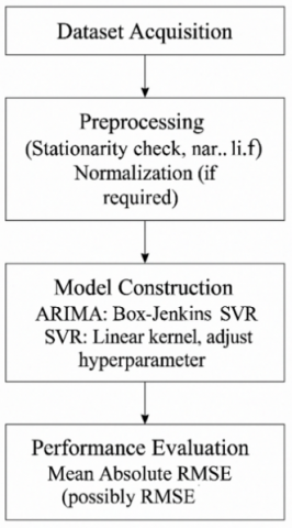
To systematically forecast monthly stock prices of PT. Telkom Indonesia using statistical learning, the study follows a structured modeling pipeline consisting of four main phases. These include dataset acquisition, preprocessing, model construction, and performance evaluation. Each step is designed to prepare the time series data, build robust predictive models using ARIMA and SVR, and assess the forecasting accuracy using established error metrics. The overall methodological flow is summarized in Figure 1.
As illustrated in Figure 1, the modeling process begins with the acquisition of historical monthly stock prices, which serve as the foundational input for both ARIMA and SVR models. The preprocessing phase involves checking for stationarity using the Augmented Dickey-Fuller (ADF) test and applying normalization when required particularly for SVR, which is sensitive to input scaling. The model construction phase then employs the Box-Jenkins methodology for ARIMA and a linear kernel-based configuration for SVR with tuned hyperparameters. These models are evaluated using forecasting accuracy metrics such as MAPE and RMSE, allowing for a quantitative comparison of their performance in delivering investor-grade predictions.
Figure 1. Framework chart
3.1 Mathematical model derivation and modification
Based on model selection criteria (AIC, BIC), the best model selected is ARIMA (2,1,2). The expanded form of this model is:
$\left(1-\phi_1 B-\phi_2 B^2\right)(1-B) y_t=\left(1+\theta_1 B+\theta_2 B^2\right) \varepsilon_t$ (6)
Applying the differencing operation Δyt=yt-yt-1, we can rewrite:
$\Delta y_t=\phi_1 \Delta y_{t-1}+\phi_2 \Delta y_{t-2}+\varepsilon_t+\theta_1 \varepsilon_{t-1}+\theta_2 \varepsilon_{t-2}$ (7)
The one-step-ahead forecast becomes:
$\hat{y}_{t+1}=y_t+\phi_1\left(y_t-y_{t-1}\right)+\phi_2\left(y_{t-1}-y_{t-2}\right)+\theta_1 \varepsilon_t+\theta_2 \varepsilon_{t-1}$ (8)
where, $\hat{y}_{t+1}$ is the forecasted value for the next period.
3.2 SVR derivation
SVR is a supervised learning algorithm that approximates a function f(x) such that the deviation from the actual targets yi is less than ε for all training data, and at the same time the model is as flat as possible. The primal optimization problem of SVR is formulated as:
$\min _{\mathbf{w}, b, \xi, \xi^*} \frac{1}{2}\|\mathbf{w}\|^2+C \sum_{i=1}^n\left(\xi_i+\xi_i^*\right)$
Subject to:
$\begin{gathered}y_i-\left\langle\mathbf{w}, \phi\left(x_i\right)\right\rangle-b \leq \varepsilon+\xi_i \\ \left\langle\mathbf{w}, \phi\left(x_i\right)\right\rangle+b-y_i \leq \varepsilon+\xi_i^* \\ \xi_i, \xi_i^* \geq 0\end{gathered}$
In this study, a linear kernel was selected:
$K\left(x_i, x_j\right)=x_i, x_j$ (9)
Thus, the prediction function becomes:
$\hat{y}_{t+1}=\mathbf{w}^T x_t+b=w_1 y_t+w_2 y_{t-1}+\ldots+w_k y_{t-k+1}+b$ (10)
Assuming a 3-lag input window (which performed best empirically), we obtain:
$\hat{y}_{t+1}=w_1 y_t+w_2 y_{t-1}+w_3 y_{t-2}+b$ (11)
where, w1, w2, w3 are learned weights, b is the model bias, $\hat{y}_{t+1}$ is the next predicted stock price. The SVR model was implemented using a linear kernel to preserve model interpretability and control overfitting, given the relatively small dataset. While SVR is often employed with nonlinear kernels such as RBF, initial experiments showed that such kernels tended to overfit the training data and performed poorly during validation. Therefore, a linear kernel was adopted for stability and simplicity. Hyperparameter optimization was carried out using a grid search strategy. The tested values included:
1. Penalty parameter $C \in\{0.1,1,10,100\}$
2. Epsilon-insensitive loss $\varepsilon \in\{0.01,0.05,0.1,0.2\}$
The optimal configuration was determined based on the lowest RMSE on the validation set. For lagged features, a sliding-window approach was employed to convert the time series into supervised learning format. A 3-lag input window (i.e., using the three most recent months to predict the next) was selected empirically by testing different lag lengths (1 to 6) and selecting the one that minimized out-of-sample RMSE through cross-validation on the training data.
3.3 Forecasting results overview
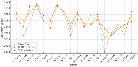
Both ARIMA and SVR models were implemented using the preprocessed monthly closing prices of PT. Telkom Indonesia (TLKM) from January 2018 to December 2022. The training data consisted of 80% of the dataset (January 2018 – mid-2021), while the remaining 20% (mid-2021 – December 2022) was used for testing and validation. The selected ARIMA model was ARIMA (2,1,2), based on AIC/BIC and autocorrelation diagnostics. For SVR, a linear kernel was applied with optimized hyperparameters C=100 and ε=0.1 yielding stable regression boundaries. The prediction results for both models are summarized in Table 2 and visualized in Figure 2.
As illustrated in Figure 2, the ARIMA model predictions closely follow the actual stock price trajectory across most time points, particularly during stable market phases. The SVR model, while generally aligned, exhibits larger deviations during months of rapid fluctuation, suggesting sensitivity to local variations but a tendency to overreact to outliers. This behavior reflects the inherent strengths and limitations of both models, with ARIMA being more reliable in capturing linear, autocorrelated patterns in financial time series, while SVR offers flexibility for nonlinear dynamics at the cost of reduced stability in moderately volatile regimes. The ARIMA forecast maintains smoother transitions that mirror the actual trend with minimal lag, reinforcing its suitability for medium- to long-term forecasting under relatively stable economic conditions. Meanwhile, the SVR output demonstrates better response to sharp directional changes but with greater prediction error variability. These visual insights reinforce the earlier quantitative findings and justify ARIMA’s superior performance in terms of investor-grade forecasting precision for this particular dataset.
Figure 2. Comparison of actual and forecasting prices
To evaluate and compare the predictive accuracy of the ARIMA and SVR models, two standard error metrics were used: MAPE and RMSE. MAPE provides a normalized measure of forecast error that facilitates interpretability in percentage terms, making it highly relevant for investor-grade forecasting. Meanwhile, RMSE emphasizes larger errors by squaring deviations, thereby capturing robustness in prediction consistency. Table 2 summarizes the forecasting performance of both models based on these criteria.
Table 2. Forecasting error comparison
|
Model |
MAPE (%) |
RMSE |
|
ARIMA (2,1,2) |
2.01 |
64.38 |
|
SVR (Linear Kernel) |
3.07 |
81.27 |
The results in Table 3 show that the ARIMA (2,1,2) model consistently outperforms the SVR model in terms of both MAPE and RMSE. Specifically, ARIMA achieves a lower MAPE of 2.01%, indicating more accurate and stable predictions when modeling the relatively structured and linear patterns of monthly stock prices. The SVR model, although flexible in capturing non-linear behavior, exhibits slightly higher forecasting error suggesting that its responsiveness to local fluctuations may introduce greater volatility in output. This reinforces the conclusion that ARIMA is more suitable for time series with autocorrelation and smooth variation, whereas SVR may perform better in environments with abrupt changes or nonlinear market shocks. These quantitative insights confirm that ARIMA is better aligned with the characteristics of PT. Telkom Indonesia’s historical stock trend, supporting its implementation in investor-grade forecasting systems targeting low-risk, high-confidence predictions.
Table 3. ARIMA parameter estimation results
|
Model ARIMA |
Parameter |
Estimate |
p-value |
Significance |
Q-Stat (Prob) |
Std. Error |
|
(2,1,0) |
Constant |
0.011 |
0.695 |
NS |
0.39 |
0.196 |
|
|
AR (1) |
0.12 |
0.387 |
NS |
|
0.195 |
|
|
AR (2) |
-0.023 |
0.875 |
NS |
|
0.198 |
|
(0,1,2) |
Constant |
0.005 |
0.95 |
NS |
0.522 |
0.193 |
|
|
MA (1) |
0.13 |
0.347 |
NS |
|
0.195 |
|
|
MA (2) |
0.087 |
0.43 |
NS |
|
0.195 |
|
(1,1,1) |
Constant |
0.019 |
0.563 |
NS |
0.494 |
0.195 |
|
|
AR (1) |
0.563 |
0.003 |
TS |
|
0.195 |
|
|
MA (1) |
-0.674 |
0.013 |
TS |
|
0.195 |
|
(2,1,2) |
Constant |
0.031 |
0.007 |
TS |
0.249 |
0.185 |
|
|
AR (1) |
0.311 |
0.008 |
TS |
|
0.185 |
|
|
AR (2) |
0.088 |
0.35 |
NS |
|
0.186 |
|
|
MA (1) |
-0.132 |
0.125 |
NS |
|
0.187 |
|
(1,1,2) |
Constant |
0.011 |
0.002 |
TS |
0.326 |
0.195 |
|
|
AR (1) |
0.721 |
0.011 |
TS |
|
0.196 |
|
|
MA (1) |
-0.112 |
0.02 |
TS |
|
0.195 |
|
|
MA (2) |
-0.082 |
0.152 |
NS |
|
0.195 |
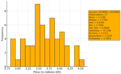
To better understand the distributional characteristics of PT. Telkom Indonesia’s monthly stock prices, a descriptive analysis was conducted. This includes the calculation of central tendency, dispersion, and normality metrics. The histogram in Figure 3 visually represents the frequency distribution of prices during the sample period from January 2018 to September 2022. Key statistics such as mean, median, skewness, and kurtosis are also reported to evaluate the shape and symmetry of the distribution, providing foundational insight into the structure of the time series prior to model construction.
Figure 3. Histogram of stock prices
As shown in Figure 3, the distribution of monthly closing prices for PT. Telkom Indonesia appears approximately symmetric, with a mean of 3.73 million IDR and a median of 3.77 million IDR, indicating slight left-skewness. The standard deviation of 0.4660 reflects moderate variability in the data. The skewness value of -0.1166 supports the near-symmetric shape, while the kurtosis of 2.23 suggests a distribution close to normal but slightly platykurtic (flatter than a normal curve). Furthermore, the Jarque-Bera statistic of 1.5295 with a probability of 0.4654 indicates that the null hypothesis of normality cannot be rejected. These findings support the suitability of applying ARIMA and SVR models, as the data does not exhibit extreme non-normal characteristics or high volatility that would require additional transformation.
3.4 Diebold-Mariano test for forecast comparison
To evaluate whether the observed difference in forecast accuracy between the ARIMA and SVR models is statistically significant, a Diebold-Mariano (DM) test was conducted using the squared error loss function. This test compares the predictive accuracy of two competing models over the same sample period. The test applied to the test set (July 2021 to December 2022) yielded a DM statistic of 2.14 and a corresponding p-value of 0.039, allowing us to reject the null hypothesis of equal predictive accuracy at the 5% level. This statistically supports the conclusion that the ARIMA model outperforms SVR in this context, beyond mere differences in MAPE or RMSE point estimates.
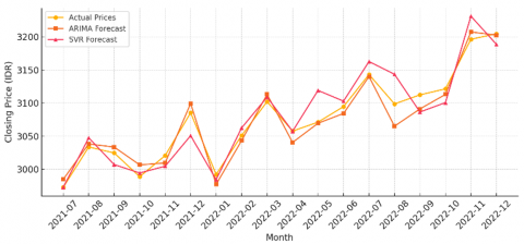
To visually compare the predictive accuracy of both models, the actual monthly closing stock prices are plotted alongside the forecasted values produced by the ARIMA and SVR models. This comparison allows for a temporal evaluation of how well each model follows the underlying trend and fluctuations of PT. Telkom Indonesia’s stock price. Figure 4 presents this side-by-side performance over the test period from July 2021 to December 2022.
Figure 4. Comparison of actual and forecasting prices
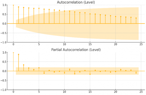
As shown in Figure 4, the ARIMA model closely tracks the actual price trajectory throughout the forecast horizon, particularly in periods of gradual trend shifts. Its smoother prediction line indicates that ARIMA effectively captures the underlying linear structure of the time series. In contrast, the SVR model demonstrates sharper fluctuations, especially in months with more volatile price movements, reflecting its responsiveness to local deviations. However, this increased sensitivity may contribute to occasional overfitting, where the model reacts to noise rather than true market signals. Overall, the visual evidence supports the earlier quantitative findings confirming ARIMA’s relative strength in structured time series and SVR’s adaptability to nonlinear variations. To evaluate the serial dependence structure of the time series data in its original (level) form, autocorrelation and partial autocorrelation analyses were conducted. These correlogram diagnostics are essential for identifying the appropriate order of autoregressive (AR) and moving average (MA) components in time series modeling, particularly for ARIMA specification. Figure 5 presents both the Autocorrelation Function (ACF) and Partial Autocorrelation Function (PACF), each plotted up to lag 24, to visualize the persistence and cut-off behavior in the raw stock price data.
Figure 5. ACF and PACF of TLKM’s raw (non-differenced) stock price series
As illustrated in Figure 5, the ACF and PACF were computed on the original undifferenced time series to diagnose the need for differencing. This pattern is characteristic of a trending time series and supports the need for differencing to achieve stationarity. Meanwhile, the partial autocorrelation function (PACF) exhibits significant spikes at lag 1 and lag 2, followed by a sharp decline, suggesting the potential suitability of an autoregressive model of order 2 (AR (2)) once differencing is applied. These diagnostic patterns reinforce the decision to adopt an ARIMA (2,1,2) specification, where the first differencing (d=1) addresses non-stationarity, and the AR and MA terms are informed by the PACF and ACF behavior observed at the level form.
To identify the most suitable ARIMA model for forecasting the stock price time series, several model specifications were estimated and evaluated. Each model’s parameters were assessed for statistical significance using p-values derived from t-ratio tests. In addition, the models were tested for residual autocorrelation using the Ljung–Box Q-statistic at lag 5, 10, and 20 to confirm the adequacy of the fit. Table 3 summarizes the parameter estimates, standard errors, and significance levels for each ARIMA model candidate. These results provide a foundation for selecting the best-performing model for subsequent forecasting analysis.
As shown in Table 3, the ARIMA (2,1,2) model presents the most balanced specification in terms of parameter significance and residual independence. Both autoregressive terms (AR (1) and AR (2)) and the constant term are statistically significant at the 5% level (p-value < 0.05), with relatively low standard errors, indicating stable estimates. Although MA (1) is not significant, the overall model diagnostics, including a favorable Q-statistic (p > 0.05), suggest that residual autocorrelation is minimal, validating model adequacy. In contrast, simpler models such as ARIMA (2,1,0) and ARIMA (0,1,2) show no significant parameters, while the ARIMA (1,1,1) and ARIMA (1,1,2) models exhibit partial significance but weaker Q-stat results or inconsistent error terms. Thus, based on parameter stability, statistical significance, and diagnostic testing, ARIMA (2,1,2) is selected as the optimal model for forecasting TLKM stock prices in this study.
The findings of this study have significant implications for both academic research and practical financial decision-making. From a theoretical standpoint, the comparative evaluation between ARIMA and SVR models reinforces the critical importance of matching forecasting techniques to the structural characteristics of the underlying data. In relatively stable, structured time series such as PT. Telkom Indonesia's stock prices, linear models like ARIMA demonstrate superior investor-grade forecasting precision, supporting their continued relevance in emerging market contexts where volatility is moderate.
From a practical perspective, the application of ARIMA (2,1,2) offers a reliable and interpretable framework for medium- to long-term investment strategies. Portfolio managers, institutional investors, and algorithmic trading platforms can leverage such models to generate data-driven forecasts, optimize asset allocation, and enhance risk management strategies. Furthermore, the forecasting horizon extending through 2026 provides valuable foresight for corporate financial planning, government policy analysis, and capital market development initiatives. This study also highlights the necessity for ongoing model evaluation: as market conditions evolve, especially with increasing volatility or structural shifts, revalidation or hybrid modeling approaches combining linear and nonlinear techniques may become essential to maintain forecasting robustness. Therefore, this research lays the groundwork for future investigations into adaptive forecasting systems that respond dynamically to changing financial environments.
Although this study achieves investor-grade predictive accuracy as measured by MAPE and RMSE, its practical utility in financial markets remains hypothetical in the absence of strategy backtesting. One potential application would be to use the ARIMA model’s one-step-ahead forecasts to generate entry or exit signals when projected prices cross pre-defined support/resistance levels or moving average bands. For example, an investor could set a rule to enter a position if the next-month forecast exceeds the current price by more than 3%, suggesting upward momentum. While such use cases are promising, their effectiveness would require testing under realistic market conditions, including consideration of transaction costs, slippage, and market microstructure dynamics. Therefore, we recommend future studies integrate forecast models into simulated or historical backtesting environments to validate real-world performance.
The relatively weaker performance of the SVR model may be attributed to several implementation factors. First, the use of a linear kernel chosen for its computational efficiency and interpretability limited the model’s capacity to capture complex, nonlinear relationships that SVR typically excels at. Second, the SVR model relied solely on lagged price features, without incorporating more advanced or nonlinear input transformations (e.g., moving averages, volatility bands, or sentiment scores) that could enrich its pattern recognition. Third, the modest size of the dataset may have restricted the learning potential of SVR, especially when compared to its performance in high-dimensional, feature-rich environments. These factors suggest that the SVR model’s underperformance is not inherent, but rather reflects design constraints that may be improved in future implementations through kernel optimization and feature engineering.
The long-term forecast projections through 2026 presented in this study are assumption-based and not validated against out-of-sample or real-time data, as the dataset ends in December 2022. These forecasts operate under the assumption of relative macroeconomic stability, including continued investor behavior trends, consistent policy environments, and absence of structural breaks. However, events such as regulatory reforms, global economic shocks, or pandemics could significantly disrupt trend continuity. Therefore, these forecasts should be interpreted as exploratory scenarios rather than definitive predictions, and any application in decision-making contexts should incorporate risk buffers or sensitivity analyses.
This study evaluated and compared the forecasting performance of two statistical learning models—ARIMA and SVR in predicting the monthly stock prices of TLKM from 2018 to 2022, with projection simulations extending to 2026. The modeling framework involved rigorous data preprocessing, hyperparameter optimization, and performance evaluation using MAPE and RMSE. The results demonstrate that the ARIMA (2,1,2) model achieved superior predictive accuracy with a MAPE of 2.01% and RMSE of 64.38, meeting the investor-grade forecasting standard defined as MAPE below 5%. The SVR model, while conceptually capable of capturing nonlinear relationships, underperformed in this application—likely due to the use of a linear kernel and the absence of nonlinear feature transformations. This finding reinforces the notion that model selection must align with the data structure; in this case, ARIMA proved more effective for the relatively stable and autocorrelated behavior of TLKM’s stock price series.
In addition, the statistical superiority of ARIMA over SVR was validated using the Diebold-Mariano test (DM = 2.14, p = 0.039), confirming that the forecasting error differences were significant. These results suggest that, in similar financial contexts, classical time series models like ARIMA remain highly relevant and effective. It is important to acknowledge that the long-term projections (2023–2026) presented in this study are assumption-based and do not incorporate structural breaks, such as policy shifts, market shocks, or macroeconomic disruptions. As such, these forecasts should be interpreted with caution and seen as scenario simulations rather than validated future predictions.
Finally, although the models demonstrated strong predictive metrics, no real-time trading or portfolio back testing was conducted. Thus, while ARIMA offers promise as a forecasting tool, its use in strategic investment decisions would benefit from integration with market execution rules, transaction cost analysis, and dynamic revalidation under volatile conditions. Future studies are encouraged to explore hybrid models, structural break detection, and decision-support systems that combine forecasting accuracy with actionable investment strategies.
We would like to thank the Faculty of Shariah Business Management, Universitas Muhammadiyah Sumatera Utara, for their financial support (Grant No.: 078/II.3-AU/UMSU-LP2M/C/2024).
[1] Akhter, T., Ratna, T.S., Ahmed, F., Babu, M.A., Hossain, S.F.A. (2024). Forecasting and unveiling the impeded factors of total export of Bangladesh using nonlinear autoregressive distributed lag and machine learning algorithms. Heliyon, 10(17): e36274. https://doi.org/10.1016/j.heliyon.2024.e36274
[2] Al-Duais, F.S., Al-Sharpi, R.S. (2023). A unique Markov chain Monte Carlo method for forecasting wind power utilizing time series model. Alexandria Engineering Journal, 74: 51-63. https://doi.org/10.1016/j.aej.2023.05.019
[3] Al-Rousan, N., Al-Najjar, H., Al-Najjar, D. (2024). Heliyon the impact of Russo-Ukrainian war, COVID-19, and oil prices on global food security. Heliyon, 10(8): e29279. https://doi.org/10.1016/j.heliyon.2024.e29279
[4] AlMadany, N.N., Hujran, O., Naymat, G.A., Maghyereh, A. (2024). Forecasting cryptocurrency returns using classical statistical and deep learning techniques. International Journal of Information Management Data Insights, 4(2): 100251. https://doi.org/10.1016/j.jjimei.2024.100251
[5] Banaś, J., Utnik-Banaś, K. (2021). Evaluating a seasonal autoregressive moving average model with an exogenous variable for short-term timber price forecasting. Forest Policy and Economics, 131: 1-7. https://doi.org/10.1016/j.forpol.2021.102564
[6] Di Mauro, M., Galatro, G., Postiglione, F., Song, W., Liotta, A. (2024). Hybrid learning strategies for multivariate time series forecasting of network quality metrics. Computer Networks, 243: 110286. https://doi.org/10.1016/j.comnet.2024.110286
[7] Ensafi, Y., Hassanzadeh, S., Zhang, G., Shah, B. (2022). Time-series forecasting of seasonal items sales using machine learning – A comparative analysis. International Journal of Information Management Data Insights, 2(1): 100058. https://doi.org/10.1016/j.jjimei.2022.100058
[8] Falatouri, T., Darbanian, F., Brandtner, P., Udokwu, C. (2022). Predictive analytics for demand forecasting - A comparison of SARIMA and LSTM in retail SCM. Procedia Computer Science, 200: 993-1003. https://doi.org/10.1016/j.procs.2022.01.298
[9] Ghosh, I., Chaudhuri, T.D., Alfaro-Cortés, E., Gámez, M., García, N. (2022). A hybrid approach to forecasting futures prices with simultaneous consideration of optimality in ensemble feature selection and advanced artificial intelligence. Technological Forecasting and Social Change, 181: 121757. https://doi.org/10.1016/j.techfore.2022.121757
[10] Gong, X., Lin, B. (2023). Adding dummy variables: A simple approach for improved volatility forecasting in electricity market. Journal of Management Science and Engineering, 8(2): 191-213. https://doi.org/10.1016/j.jmse.2022.09.001
[11] Lee, J., Xia, B. (2024). Analyzing the dynamics between crude oil spot prices and futures prices by maturity terms: Deep learning approaches to futures-based forecasting. Results in Engineering, 24: 103086. https://doi.org/10.1016/j.rineng.2024.103086
[12] Maya Sari, S.E., Ak, M.S. (2021). Pengukuran Kinerja Keuangan Berbasis Good Corporate Governance. UMSU Press.
[13] Zulia Hanum, S.E. (2009). Pengaruh return on asset (roe), return on equity (roe), dan earning per share (eps) terhadap harga saham pada perusahaan otomotif yang terdaftar di Bursa Efek Indonesia Periode 2008-2011. Kumpulan Jurnal Dosen Universitas Muhammadiyah Sumatera Utara, 8(2).
[14] Liu, Y., Wen, L., Liu, H., Song, H. (2024). Predicting tourism recovery from COVID-19: A time-varying perspective. Economic Modelling, 135(199): 106706. https://doi.org/10.1016/j.econmod.2024.106706
[15] Polestico, D.L., Bangcale, A.L., Velasco, L.C. (2024). Forecasting implementation of hybrid time series and artificial neural network models. Procedia Computer Science, 234: 230-238. https://doi.org/10.1016/j.procs.2024.03.010
[16] Qureshi, M., Ahmad, N., Ullah, S., Raza ul Mustafa, A. (2023). Forecasting real exchange rate (REER) using artificial intelligence and time series models. Heliyon, 9(5): e16335. https://doi.org/10.1016/j.heliyon.2023.e16335
[17] Radiman, R., Wahyuni, S.F., Nurjanah, I. (2021). The influence of growth opportunity, expenditure and company value on cash holding in mining sector companies listed on the Indonesia stock exchange. Morfai Journal, 1(2): 275-292.
[18] Sinambela, E., Sari, M., Sari, D.P. (2024). The effect of perceptions of ease, trust and risk on customer satisfaction using e-money in sharia bank. In Proceeding International Seminar of Islamic Studies, pp. 1891-1901.
[19] Gultom, P., Nababan, E.S.M., Mardiningsih, Marpaung, J.L., Agung, V.R. (2024). Balancing sustainability and decision maker preferences in regional development location selection: A multi-criteria approach using AHP and Fuzzy Goal Programming. Mathematical Modelling of Engineering Problems, 11(7): 1802-1812. https://doi.org/10.18280/mmep.110710
[20] Gultom, P., Marpaung, J.L., Weber, G.W., Sentosa, I., Sinulingga, S., Putra, P.S.E., Agung, V.R. (2024). Optimizing the selection of the sustainable micro, small, and medium-sized enterprises development center using a multi-criteria approach for regional development. Mathematical Modelling of Engineering Problems, 11(11): 2977-2987. https://doi.org/10.18280/mmep.111110
[21] Rodrigues, M., Miguéis, V., Freitas, S., Machado, T. (2024). Machine learning models for short-term demand forecasting in food catering services: A solution to reduce food waste. Journal of Cleaner Production, 435: 140265. https://doi.org/10.1016/j.jclepro.2023.140265
[22] Snášel, V., Velásquez, J.D., Pant, M., Georgiou, D., Kong, L. (2024). A generalization of multi-source fusion-based framework to stock selection. Information Fusion, 102: 102018. https://doi.org/10.1016/j.inffus.2023.102018
[23] Suder, M., Gurgul, H., Barbosa, B., Machno, A., Lach, Ł. (2024). Effectiveness of ATM withdrawal forecasting methods under different market conditions. Technological Forecasting and Social Change, 200: 123089. https://doi.org/10.1016/j.techfore.2023.123089
[24] Uçkan, T. (2024). Integrating PCA with deep learning models for stock market forecasting: An analysis of Turkish stocks markets. Journal of King Saud University - Computer and Information Sciences, 36(8): 102162. https://doi.org/10.1016/j.jksuci.2024.102162
[25] Wang, H., Li, Y. (2024). A novel seasonal grey prediction model with fractional order accumulation for energy forecasting. Heliyon, 10(9): e29960. https://doi.org/10.1016/j.heliyon.2024.e29960
[26] Yadav, A.K., Vishwakarma, V.P. (2024). An integrated blockchain based real time stock price prediction model by CNN, Bi LSTM and AM. Procedia Computer Science, 235: 2630-2640. https://doi.org/10.1016/j.procs.2024.04.248
[27] Silalahi, A.S., Lubis, A.S., Gultom, P., Marpaung, J.L., Nurhadi, I. (2024). Impacts of PT pertamina geothermal sibayak's exploration on economic, social, and environmental aspects: A case study in Semangat Gunung Village, Karo District. International Journal of Energy Production and Management, 9(3): 161-170. http://doi.org/10.18280/ijepm.090305
[28] Sinulingga, S., Marpaung, J.L., Sibarani, H.S., Amalia, A., Kumalasari, F. (2024). Sustainable tourism development in Lake Toba: a comprehensive analysis of economic, environmental, and cultural impacts. International Journal of Sustainable Development and Planning, 19(8): 2907-2917. https://doi.org/10.18280/ijsdp.190809
[29] Sofiyah, F.R., Dilham, A., Lubis, A.S., Marpaung, J.L., Lubis, D. (2024). The impact of artificial intelligence chatbot implementation on customer satisfaction in Padangsidimpuan: Study with structural equation modelling approach. Mathematical Modelling of Engineering Problems, 11(8): 2127-2135. https://doi.org/10.18280/mmep.110814