Abdul-Sahib T. Al-Madhhachi*![]() | Mohammed A. Jameel
| Mohammed A. Jameel![]() | Haider A. Al-Mussawy
| Haider A. Al-Mussawy![]() | Faris W. Jawad
| Faris W. Jawad![]()
© 2025 The authors. This article is published by IIETA and is licensed under the CC BY 4.0 license (http://creativecommons.org/licenses/by/4.0/).
OPEN ACCESS
Typically, subsurface flow influences the erosion of dams, hillslopes, embankments, streambeds and banks. To enhance forecasts of the erosion rate of cohesive streambanks, recent studies integrated subsurface flow into a mechanical fundamental erosion rate model known as “Adapted Wilson Model”. The recent mechanistic erosion model has the ability to predict erosion rates under the subsurface flow based on two adapted dimensional soil parameters (b0 and b1), where b0 is the first Wilson detachment term, and b1 is the second Wilson detachment term, at different applied hydraulic gradients. However, this model was not yet applied to field data in the presence of subsurface flow in streambanks. The aim of this research was to use “Adapted Wilson Model” parameters (b0 and b1) to predict the influence of subsurface flow on erosion of Cow Streambanks located in Oklahoma, USA at different applied hydraulic gradients. A miniature version of the Jet Erosion Test device (mini-JET) was utilized in situ to derive the parameters, b0 and b1, of Cow Streambanks. The observed data for Cow Streambanks was predicted by the "Adapted Wilson Model," and the results were compared with those obtained in laboratory settings. As a function of subsurface flow gradient and density, subsurface flow had an uneven impact on b0 and b1 in both observed and predicted erosion data. The "Adapted Wilson Model" parameters can be used to forecast the impact of subsurface flow in both laboratory setups and field data using JET methods.
cohesive soil, detachment rate model, cow stream, jet erosion test, surface and subsurface flow
Around the world, streambank and hillslope erosion are significant geomorphologic processes. Indeed, in certain streams, streambank erosion accounts for a sizable portion of the overall sediment load [1-3]. In cohesive soils, destabilizing and streambank breakdown or failure are frequently caused by streambank erodibility near the bank toe or at the top of confining strata [4]. Additionally, during and right after storm events, the groundwater and streamflow have a substantial interaction close to some spots at streambank. However, the interaction between surface forces and nearby subsurface groundwater forces, particularly their impact on surface erosion, is typically overlooked when calculating surface erosion rates [4].
The significance of subsurface flow on erosion and bank or hillslope failure has been shown in a number of studies [4-6]. Subsurface flow-specific erosion has been the subject of numerous investigations, including the development of practical deposit conveyance models for this spectacle [6-10]. Another field subsurface flow studies have highlighted the complex relationship between subsurface flow and surface forces [11]. However, further research is required to fully comprehend how groundwater seepage gradients contribute to surface erosion. Usually, the Bank Stability and Toe Erosion Model (BSTEM) were used to simulate the erosion rate of cohesive streambanks [11] using excess shear stress equation. The absence of mechanistic predictions of an excess shear stress model’s parameter for specific soil and flow conditions is a drawback when taking into account different forces impacting soil erosion. The variety of environmental circumstances encountered during surface erosion is best modeled using a more primarily based, mechanical erodibility model. The method for directly adding subsurface flow is a mechanistic erosion model.
Wilson developed [12, 13] a mechanical erodibility model (Wilson Model) to offer a comprehensive framework for researching the properties of fluids and soils and how they affect cohesive soil erosion. A basic two-dimensional representation of particles served as the basis for the development of the model. Nevertheless, the erosion model can be used for aggregates and is not restricted to a soil single particle. Data on cohesive soil erosion rates were used to assess the model. Two dimensional parameters, b0 and b1, where b0 is the first Wilson detachment term, and b1 is the second Wilson detachment term, were used to calibrate the model to the observed scour depth data.
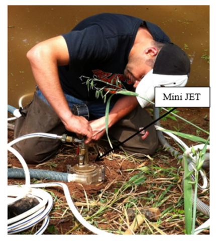
A mini-JET apparatus, which is a small-scaled version of the Jet Erosion Test, was produced [14]. The mini-JET device is easier to use in the field and in the lab because it is lighter, smaller, and uses less water compared to the original JET device. Results from the mini-JET are nearly identical to those from the regular JET [15, 16]. In order to forecast the erosion of cohesive soils, Al-Madhhachi et al. [15] integrated the hydraulic analysis of JET devices into the Wilson Model, a basic detachment model. They used both the original and mini-JET machines, and they used data from flume testing to confirm the results. For flume and JET devices, the "Wilson Model" predicted the observed data as well as or better than the excess shear stress model (linear model). The "Wilson Model" and the linear model parameters can be used to forecast the rate of cohesive soil erosion. Al-Madhhachi et al. [15] confirmed the results of using mini-JET with the flume test results using both models. They came to the conclusion that the excess shear stress equation could be replaced with the more fundamentally based erosion model, whose parameters could be determined using current JET methods.
In order to estimate the dimensional mechanistic erosion parameters, b0 and b1, Al-Madhhachi et al. [17] integrated Iraqi stabilizers into the basic context of Wilson Model. The findings demonstrate that for all stabilizers and cured polluted soils at various preserving times, the observed parameter b1 values rose. For the preserved polluted soils, the measured b0 dramatically dropped with increasing curing time. To ascertain the mechanical soil erodibility parameters (b0and b1) of the Wilson Model, Abbood and Al-Madhhachi [18] used a JET apparatus on undisturbed soil samples of crusted and uncrusted soils obtained from Tigris Riverbanks and air dried at various curing times. The value b0 for crusted soils decreased by 60% after 14 days of curing, while the factor b0 for uncrusted soil increased by 90% after 21 days. Their research demonstrates how using a JET device can shorten testing durations, conserve energy, and offer an inexpensive way to monitor crusted soil stability.
In order to forecast the erosion of cohesive soils, Al-Madhhachi et al. [19, 20] integrated subsurface flow into a mechanistic erosion model. Their model (Adapted Wilson Model) contained subsurface flow with two soil parameters (b0and b1) and was constructed on the overall agenda created by Wilson [12, 13]. They laboratory measured the "Adapted Wilson Model" parameters (b0and b1) for two alternative soils packed at specific density close to the soil's optimal water content using open channel flow and mini-JETs in addition to a subsurface flow column. With previous JET studies without subsurface flow, Al-Madhhachi et al. [19, 20] discovered that the impact of subsurface flow on erodibility may be forecasted using JET procedures in the "Adapted Wilson Model" equations. However, Al-Madhhachi et al. [19, 20] did not forecast the impact of subsurface flow on field data, and their model was restricted to laboratory testing only. Thus, the goal of this study was to use the mini-JET device to forecast the impact of subsurface flow at different hydraulic gradients on erosion of Cow Streambanks in Oklahoma using the "Adapted Wilson Model" equations b0and b1, and the results were compared with the laboratory data that performed by studies [19, 20]. The benefit of the proposed model is the ability to predict the soil erosion of streambanks that are suffering from seepage flow and fluvial erosions at the same time by applying the mini-JET on streambanks without seepage.
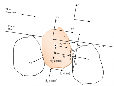
The for-particle detachment, the removing and steadying forces and their corresponding moment distances served as the general basis for estimating erosion rate [12]. The lift force (LF), drag force (DF), particle weight (ws), contact forces between particles (Cf1, Cf2, …, Cfn), and the additional subsurface flow force (Sf) are all conceptually depicted in Figure 1 as the forces that performance to detach a soil particle. If the driving moment exceeds resisting moment, particle separation takes place [12]. These moments proceeded around point A, according to Wilson [12]. When subsurface flow force is added, the point of emerging indication can be described as follows:
$\begin{aligned} & D_F\left(l_3\right)+L_F\left(l_4\right)+w_s \sin (\alpha)\left(l_1\right)+S_f \cos \alpha\left(l_2\right) \\ & \quad=w_s \cos (\alpha)\left(l_2\right)+S_f \sin \alpha\left(l_2\right)+C_M\end{aligned}$ (1)
Figure 1. Subsurface flow force acting on a single soil particle in open channel bed with other forces
where, $w_s=g\left(\rho_s-\rho_w\right) V_k d^3$ is the weight of the underwater particle; $\rho_s= 2.65 \mathrm{Mg} / \mathrm{m}^3$ is the particle bulk density $[21]$; $\rho_w=1 \mathrm{Mg} / \mathrm{m}^3$ is the water density; $V_k\left(=\frac{\pi}{6}\right)$ is the volume constant of a spherical particle; $d$ is the corresponding particle diameter; $S_f=H_i V_k d^3 g \rho_w$ is the force acting beneath the surface of a single particle; $C_M$ is the total of the frictional forces moments of cohesive particle [12], $H_i=H / L$ is the hydraulic gradient, $H$ is a subsurface flow head, $L$ is the soil length, $l_1$, $l_2$, $l_3$, $l_4$, and $l_5$ are lengths of moments for the forces, and $\alpha$ is the slope of the channel angle. Eq. (1) can be rewritten as follows by applying the subsurface force formula and assuming that the lift and drag forces are proportionate (i.e., $L_K / F_K=L_F / D_F$) [12, 19, 22]:
$D_F=w_s\left(K_{l s}-S_K+C_{f c}\right)$ (2a)
$K_{l s}=\frac{\cos (\alpha)\left(l_2-l_1 S\right)}{l_3+l_4 \frac{L_K}{F_K}}$ (2b)
$S_K=\frac{H \rho_w}{L\left(\rho_s-\rho_w\right)} \frac{\cos (\alpha)\left(l_2-l_5 S\right)}{l_3+l_4 \frac{L_K}{F_K}}$ (2c)
$C_{f c}=\frac{C_M}{w_s\left(l_3+l_4 \frac{L_K}{F_K}\right)}$ (2d)
where, $S_K$ is a subsurface term that based on hydraulic gradient, particle bulk density, positioning within the channel bed, and grade; $K_{l s}$ is a dimensionless parameter that based on size of particle, alignment within the channel bed, and grade [12]; $L_K=1$ is the ratio of lift to drag factors [12, 13]; $C_{f c}$ is a cohesion parameter; $F_K$ is the proportion of projected area lift to drag forces; and $S$ is the channel bed slope.
If the hydraulic properties on the left-hand side $\left(D_F\right)$ of Eq. (2a), which is mostly determined by subsurface flow, particle, and bed properties, is larger than the other side, $w_s\left(K_{l s}-S_K+C_{f c}\right)$, the particle gets detached. For spherical particles with similar radii, Wilson [13] proposed that the moment lengths are $l_1=0.86 \mathrm{~d} / 2, l_2=l_4=0.5 \mathrm{~d} / 2$, and $l_3=1.18 \mathrm{~d} / 2$. These moment distances were calculated using Wilson's [13] particle size and gap combinations. The moment distance of the horizontal element of the subsurface flow force, or the new moment length $l_5=0.14 \mathrm{~d} / 2$. Likewise, Wilson [13] proposed that parameter $F_k$ has a value of 0.92 for equal radii of a spherical soil particle created on the grouping of particle volumes and openings.
When the force of drag in Eq. (2a) exceeds the weight, cohesion, and subsurface flow forces, particle detachment takes place. Due to limited information on these parameters (including $C_{f c}$ and $E_K$, where it is the parameter of exposure), Al-Madhhachi et al. [19, 20] utilized an adjustment process to get term values, in accordance with the Wilson [12, 13] framework. Al-Madhhachi [19, 20] created a unique method to calculate the overall erosion rate by indirectly including the effects of soil particle volumes in the adjustment processes since it was difficult to detect the interface between soil particle volumes when the entire erodibility rate was involved. Using the same methodology as Wilson [12, 13], dimensional parameters $b_0$ and $b_l$ are created to express the total erodibility rate, $D_r$, in the presence of subsurface flow as follows:
$D_r=b_0 \sqrt{\tau}\left[1-\exp \left\{-\exp \left(3-\frac{b_1}{\tau}\right)\right\}\right]$ (3a)
$b_0=\rho_s \frac{R_K}{E_K} \sqrt{\frac{N_K+S_{K t}}{D_{k k}\left(\rho_s-\rho_w\right)}}$ (3b)
$b_1=\left(\frac{\pi}{e_v \sqrt{6}}\right) \frac{R_K\left(K_{l s}-S_K+C_{f c}\right)}{K_o} g\left(\rho_s-\rho_w\right) d$ (3c)
$S_{K t}=\frac{\mu_s g H_i d \rho_w}{\tau}=\mu_{s r} g H_i d \rho_w$ (3d)
where, $b_0$ is the first Wilson erosion term, and $b_1$ is the second Wilson detachment term. The subsurface flow coefficient ratio is denoted by $S_{K t}$, which is the subsurface flow parameter resulting from a particle's exchange time. As the soil erodes, observe that it rises and falls. However, according to experimental data from JETs and flume tests published in Al-Maddhachi et al. [19,20], the value of $\mu_{s r}=3.85$. Eqs. (3a) through (3d) are referred to as the "Adapted Wilson Model" in this study. A method for fitting curves using Microsoft Excel Solver was used to reduce the errors in the estimated parameters compared to the recorded erodibility data, allowing for the calculation of parameters $b_0$ and $b_1$ with error metrics below 0.001. When there is no subsurface flow, the subsurface flow parameters (i.e., $S_K=0$ and $S_{K t}=0$) can be disregarded, and the generated model will correspond to the Wilson equations [12, 13]. JETs [23] and flume testing are two popular techniques for producing data to determine the erosion terms of the "Adapted Wilson Model".
3.1 Study area and materials
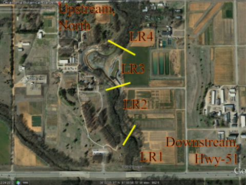
In the US, streambank stabilization and restoration are common practices. However, there is currently a dearth of information regarding how construction methods affect a streambank's ability to withstand surface erosion and geotechnical failure. The location will be monitored and studied for at least five years after along Cow Stream, Oklahoma, USA. Oklahoma State University constructed a multidisciplinary center for streambank and riparian research, instruction, and demonstration. Cow Stream is a representative Oklahoma Greek that has had its natural course altered. As a result, the stream is currently growing wider and deeper, and related side-gullies are forming (Figure 2). To calculate the bo and b1 of Wilson Model from site data, mini-JETs (Figure 3) were carried out on the Cow Streambanks. The details of the setup and operation of the mini-JET were previously explained in previous research [14-20]. As realized in Figure 2, the JETs were approved as portion of a Greek restoration scheme beside four reaches (LR1, LR2, LR3, and LR4) with varying degrees of streambank modification. JETs without subsurface flow at the time were used to determine the bo and b1 of the "Adapted Wilson Model". For a number of fictitious subsurface flow gradients, the soil erosion of LR3 reach was also examined.
The Cow Streambanks restoration project was suffering from seasonal floods that caused the streambank to erode, and a future failure may occur in existing structures, especially in the reach between sections LR3 and LR4. In addition, section LR3 was suffering from local groundwater flow forces. As part of the restoration project, Cow Stream was investigated in four reaches. Impact on erosion characteristics and processes was compared between these reaches, includes new development in the strongly adapted reach, two downstream reaches with built rock structures, and exchanges with the non-impacted plant assemblage at the control site upstream of the project. At the first reach (LR1), which is located upstream of the highway (Figure 2), a downstream double-step cross-vane was positioned on the downstream side of the meander bend, while a J-hook was positioned on the upstream side of the inner meander bend region.
Erosion matting and seed were used to stabilize this area. After construction, the top disturbed areas were once more restored with vegetation plantings, straw mulch, and seed. Due to the excavation and filling of the benches, stream bank slopes, and the altered stream alignment, the third reach (LR3) has undergone the biggest modification. There are no rock formations in the downstream portion of this stretch. Six sites of 180-meter-long research with 1H:1V slopes are situated along the stream in LR3. Construction did not disrupt the final reach (LR4).
Figure 2. Four reaches located in Cow Stream, Oklahoma, USA
Figure 3. In – field mini-JET apparatus located in Cow Streambanks, Oklahoma, USA
Table 1. Soil properties of four reaches in Cow Streambanks, Oklahoma
|
Soil Characteristics |
Reaches |
|||
|
LR1 |
LR2 |
LR3 |
LR4 |
|
|
Sand (%) |
45 |
55 |
57 |
52 |
|
Silt (%) |
25 |
22 |
20 |
22 |
|
Clay (%) |
27 |
24 |
24 |
27 |
|
Water Content (%) |
19-23 |
16-18 |
12-21 |
13-29 |
|
Dry Density (Mg/m3) (average values) |
1.26-1.42 (1.34) |
1.54-1.72 (1.56) |
1.58-1.88 (1.72) |
1.42-1.62 (1.59) |
From every reach, soil samples were gathered and examined (Table 1). ASTM Standards 2006 were followed in the testing and analysis of these samples. At Oklahoma State University's Soil Laboratory, Hydrometer testing and sieve examination were achieved in compliance with ASTM Standard D422. The soil samples' dry densities and water contents were calculated (Table 1).
3.2 Predicting subsurface flow erosion from field mini-JETs
For distinguishable soil deposits, in situ mini-JETs were carried out at the three management locations (LR1, LR2, and LR3) as well as the upstream control site LR4. Using the generalized reduced gradient method, an iterative process is used to reduce the error between the functional solutions of the equation and the observed data, the "Wilson Model" parameters bo and b1 were determined created on erosion data from mini-JETs. The "Adapted Wilson Model" parameters (Eqs. (3b) and (3c)) were used to examine the impact of subsurface flow on the erodibility of streambanks at reach LR3. The "Adapted Wilson Model" parameters from laboratory tests were compared to the one calculated from the field data because both tests were used the silty sand soil that acquired from reach LR3 [14].
To study the influence of subsurface flow on erosion terms in both configurations, an example of a JET versus flume data analysis was provided. Eq. (3c) of modified parameter b1 can be recast as follows for open channel flow tests:
$b_1=\left(\frac{\pi}{e_v \sqrt{6}}\right) \frac{R_K\left(K_{l s}+C_{f c}\right)}{K_o} g\left(\rho_s-\rho_w\right) d-\left(\frac{\pi}{e_v \sqrt{6}}\right) \frac{R_K S_K}{K_o} g\left(\rho_s-\rho_w\right) d$ (4)
where, the first term in Eq. (4) is the term $b_1$ of the "Wilson Model" from open channel flow data in absence of subsurface flow. It was supposed that the particle was tetragonal, as suggested by Al-Maddhachi et al. [19, 20]. The following assumptions or conclusions can be used to quantitatively calculate the other term of Eq. (4): $S_K$ based on subsurface flow gradient $H_i$; the moments distances, $l_1=0, l_2=l_4=d / 2$, and $l_3=l_5=P_n d / 2$ for a tetragonal particle; $F_K\left(=a_k / P_n\right.$, where $\left.a_k=1\right)$; $\rho_s=2.65 \mathrm{Mg} / \mathrm{m}^3$; $\rho_w=1 \mathrm{Mg} / \mathrm{m}^3$; $d=0.16 \mathrm{~mm}$; the open channel velocity parameter, $K_o=\frac{\left[C_D F_K\left(\frac{1}{k_s} \ln \left(z_d\right)+B\right)^2\right]}{2}$, depends on $C_D=0.2$ according to the reference [24]; von Karmon $k=0.4$; $k_s$ is a roughness height equal to $\left(P_n d / 2\right)$ for a tetragonal particle; $z_d\left(=l_3+y_p\right)$, where $y_p=0$; and $B=6.5$.
The modified parameter $b_1$ from Eq. (3c) can also be represented as Eq. (4) for JET data. Where the "Wilson Model" parameter $b_1$ from JET data without subsurface flow is the first term in Eq. (4) $\left(\frac{\pi}{e_v \sqrt{6}}\right) \frac{R_K\left(K_{l s}+C_{f c}\right)}{K_o} g\left(\rho_s-\rho_w\right) d$. The following assumptions or conclusions can be used to quantitatively calculate the second term in Eq. (4): The velocity parameter for JET, $K_o=\frac{5.537 C_D F_K \exp \left[-200\left(\frac{z_d}{r}\right)^2\right]}{C_f D_c{ }^2}$, is dependent on the following: $C_f=0.00416$; $r=0.13 J_i$ according to references [14, 15]; $z_d\left(=l_3+y_p\right)$, where $y_p(=0)$ for a tetragonal particle; $C_D=0.2$ as stated in reference [23], and $D_c=0.65$ is the discharge coefficient.
Subsurface flow parameter $S_{K t}=\mu_{s r} g H_i d \rho_w$ affects the "Adapted Wilson Model" parameter bo (see Eq. (3b)). The following assumptions or determinations can be used to mathematically determine the terms in Eq. (3b) for the flume: The subsurface flow coefficient ratio is $\mu_{s r}$ (where $\mu_{s r}=3.85$ as recommended by references [19, 20]; $N_K=T_K K_o / R_K$; $T_K=2.5$ as suggested by Chepil [22]; $D_{K K}=2$ as suggested by Einstein [25]; and other expressions were defined above. Without subsurface flow, the observed flume data can be used to forecast the parameter $E_K$:
$E_K=\rho_s \frac{R_K}{b_0} \sqrt{\frac{N_K+S_{K t}}{D_{k k}\left(\rho_s-\rho_w\right)}}$ (5)
As anticipated, variations in the "Wilson Model" parameters $b_o$ and $b_l$ were found for tests conducted utilizing in situ mini-JET along the four reaches of Cow Streambanks.
Similarly, the parameters in Eq. (3b) were computed analytically in the same way as previously described in order to forecast parameter $b_0$ for JETs. The parameter $K_o$ was the only ones that differed. The observed JET data without subsurface flow can also be used to calculate the parameter $E_K$ using observed $b_0$.
4.1 Subsurface flow example investigation
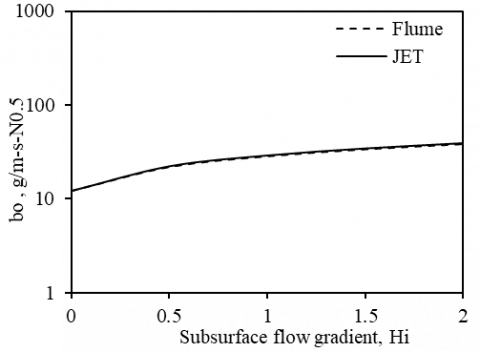
The impact of subsurface flow on cohesive soil erosion and the resultant erosion parameters with subsurface flow are illustrated through an example. The soil was analysis as 70% sand, 14% silt, and 16% clay, and defined as silty sand soil, is used as an example. Samples of distributed streambanks from Cow Stream, Oklahoma, were acquired [15, 26]. Depended on data observed from open channel flow and/or JET without subsurface flow, it is theoretically possible to forecast the soil erosion under the impact of subsurface flow, as was previously discussed. Without repeating JETs or flume tests, b1 and b0 can be established from measured or anticipated subsurface flow gradients since the parameters of the proposed model are mechanistically specified. Using optimum moisture soil samples of 14.2% and packed at 1.69 Mg/m3 without applied the influence of subsurface flow, the proposed model was able to predict subsurface flow erosion parameters [15]. This data was fitted to the "Wilson Model" (without subsurface flow) using estimated values of b0 = 12 g/m-s-N0.5 and b1= 6 Pa.
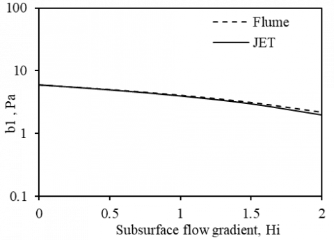
Subsurface flow altered the calculated "Adapted Wilson Model" parameters (b1 and b0) for the silty sand soil example that mentioned above (Figure 4). It should be noted that for both flume experiments and JETs, a greater subsurface flow gradient caused b0 to increase (Eq. (3b)) when parameter SKt increased. When the subsurface flow gradient was increased to around 2 m/m, the term value reformed by about one order of scale. For both open channel tests and JETs, b1 dropped as the subsurface flow force (SK) rose (Figure 4). Similarly, b1 fluctuated by almost an order of scale after the subsurface flow gradient was increased to around 200 cm/cm. As seen in Figure 4, the flume erosion data can be predicted using the JET approaches.
(a)
(b)
Figure 4. Subsurface flow gradients' effects on the parameters of "Adapted Wilson Model" for a soil of silty sand with a bulk density of 1.76 Mg/m3 and an optimum soil moisture
The data from Al-Madhhachi et al. [15] were used for no subsurface flow gradient. Predictions of b0 and b1 of the proposed model (Eqs. (3b) and (3c)) are represented by values at the different subsurface flow gradients, Hi.
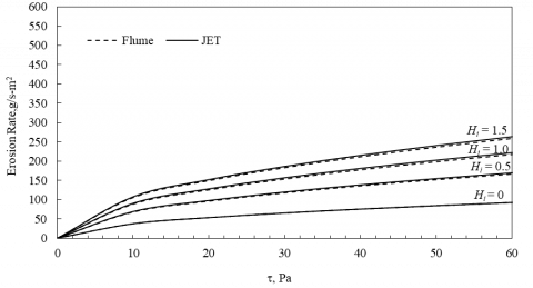
Subsurface flow results were applied on rate of soil erodibility versus applied shear stress using the parameters of the proposed model, the impact of the subsurface flow gradients was apparent (Figure 5). Once more, based on projected b0 and b1, the JET approaches yielded erosion rates that were comparable to those of flume testing. It was observed a nonlinear relationship between rates of soil erodibility versus applied shear stress when the subsurface flow gradient was equal to zero. While a linear relationship between them appears at applied shear stress of 10 Pa. However, the linear model is unable to predict this nonlinear relationship compared to proposed model (Figure 5). The aforementioned research shows how the "Adapted Wilson Model" can be used to forecast how subsurface flow will affect soil erosion.
Figure 5. Using the parameters of "Adapted Wilson Model" for open channel flow and JETs, the rate of soil erodibility versus applied shear stress of a silty sand soil is plotted for both scenarios with and without subsurface flow gradients, Hi
4.2 Predicting subsurface flow parameters from field data
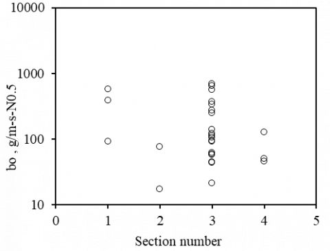
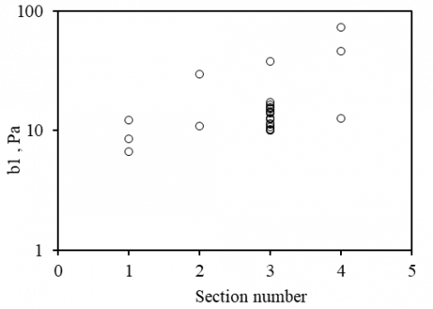
As anticipated, variations in the "Wilson Model" parameters bo and b1 were found for tests conducted utilizing in situ mini-JET along the four reaches of Cow Streambanks (Figures 6 and 7).
Figure 6. Calculating observed Wilson Model parameter bo using field JETs carried out at several reaches along Cow Greek banks, Oklahoma
Figure 7. Calculating observed Wilson Model parameter b1 using field JETs carried out at several reaches along Cow Greek banks, Oklahoma
It seems that there were no discernible changes in the reaches as a result of streambank alteration, including excavation and restoration. Although there was no association with the type of streambank modification, there was a general upward trend in parameter b1 (Figure 7). As previously mentioned, it is theoretically possible to forecast the influence of subsurface flow on soil erodibility using observed data of streambank derived from JET device without applied the subsurface flow (Eqs. (3b) and (3c)).
Nine tests on the LR3 Cow Streambank yielded an average b1 value of 13.98 Pa for this reach. With the previously specified parameters, the expressions in Eq. (3c) were computed mathematically. Similarly, subsurface flow also affects the parameter b0, especially in the SKt term (see Eq. (3b)). The previously defined values can be used to mathematically determine the terms in Eq. (3b). Using Eq. (5) and average b0 = 75.67 g/m-s-N0.5 for the nine experiments, the parameter EK may be estimated from observed outcomes of JET apparatus collected on bank of section LR3 in the absence of subsurface flow.
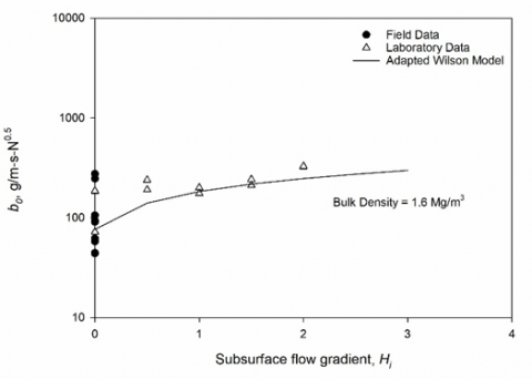
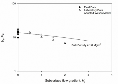
The observed results from JETs that conducted laboratory on a vertical configuration for the soil of silty sand were accurately calculated using the prediction equations for bo and b1from derived field data parameters (Figures 8 and 9). The derived parameter from mini-JET studies in laboratory setups with subsurface flow on vertical arrangement are shown by triangle symbols. The derived parameter from field mini-JETs on bank of section LR3 of Cow Greek for a scenario without subsurface flow are represented by solid circle symbols. The predictions of b1 using Eq. (3b) of proposed model based on field data using the various subsurface flow gradients (Hi) are shown by dashed lines. The "Adapted Wilson Model" could be incorporated in BSTEM to forecast soil erosion caused by surface flow and/or any additional forces, according to the results of field and laboratory data trials. A good matchup between observed laboratory data taken from study [19, 20] and the predictions parameters from Eqs. (3b) and (3c) (Figures 8 and 9). The nominal objective function (FNM) was Estimated to determine the difference between laboratory and field data. There are no differences in the results as the value of FNM approached zero. The results of the comparison between laboratory and field data indicated that FNM was equal to 0.18 for parameter b0 and 0.14 for parameter b1. Soil heterogeneity, soil texture, soil moisture content, and other environmental factors could influence the variability in b0 and b1 in the field applications compared to the laboratory setup.
Figure 8. Assessing the capability to forecast the "Adapted Wilson Model" parameter b0 derived from field data for the LR3 of Cow Greek banks, OK, using field JETs without subsurface flow
Figure 9. Assessing the capability to forecast the "Adapted Wilson Model" parameter b1 derived from field data for the LR3 of Cow Greek banks, OK, using field JETs without subsurface flow
To forecast the erodibility of cohesive streambanks, a basic erosion model was developed that included subsurface flow forces working in tandem with surface flow. The fundamental framework created by Wilson [12, 13] served as the foundation for the "Adapted Wilson Model," which further includes subsurface flow with two mechanistic soil parameters (b0 and b1). The parameters b0 and b1 of "Adapted Wilson Model" for soil of silty sand at four locations along the Cow Streambanks in Oklahoma were determined using a mini-JET device. When employing the "Adapted Wilson Model" parameters, subsurface flow had an impact on both the observed and estimated data. The observed results spanning a variety of subsurface flow gradients applied on silty sand soil were predicted by the proposed model. As anticipated, higher subsurface flow raised the parameter b0 by 81%, while decreasing in the observed and predicted parameter b1 by 50%. The proposed model has the ability to predict the soil erosion of streambanks that are suffering from seepage flow and fluvial erosions at the same time by applying the mini-JET on streambanks at the time without seepage. Compared to other models, such the linear model, the "Adapted Wilson Model" has the advantage of being a more mechanistic, fundamentally based erosion equation.
The authors acknowledge the Department of Water Resources Engineering, Mustansiriyah University (www.uomustansiriyah.edu.iq), in Iraq for their support. The authors also acknowledge Oklahoma State University for the support and performing the field and laboratory testing used this research.
|
aK |
area constant |
|
B |
constant of shear Reynolds number |
|
b0 |
first Wilson erosion term, g.m-1.s-1.N-0.5 |
|
b1 |
second Wilson detachment term, Pa |
|
CD |
drag coefficient |
|
Cf |
coefficient of friction |
|
Cf1, Cf2, …, Cfn |
contact forces between particles, N |
|
Cfc |
cohesion parameter |
|
CM |
parameter of total of the frictional forces moments of cohesive particle |
|
Dc |
discharge coefficient |
|
DF |
drag force, N |
|
DKK |
detachment distance parameter |
|
Dr |
detachment rate, g.s-1.m-2 |
|
d |
soil particle diameter, mm |
|
EK |
parameter of exposure |
|
ev |
variation parameter |
|
g |
gravity acceleration, m.s-2 |
|
FNM |
nominal objective function |
|
FK |
proportion of projected area lift to drag forces |
|
H |
subsurface flow head, cm |
|
Hi |
hydraulic gradient, cm/cm |
|
Ji |
jet nozzle height, mm |
|
Ko |
velocity parameter for flume or JET |
|
Kls |
dimensionless parameter that based on size of particle, alignment within the channel bed, and grade |
|
k |
von Karmon |
|
ks |
roughness height, mm |
|
L |
soil sample length, cm |
|
LF |
lift force, N |
|
LK |
ratio of lift to drag factors |
|
l1, l2, l3, l4, and l5 |
lengths of moments for the forces, mm |
|
NK |
combination of particle and fluid factors |
|
Pn |
length parameter of tetragonal particle |
|
RK |
geometry ratio |
|
r |
jet radius, mm |
|
Sf |
subsurface flow force, N |
|
SK |
subsurface term that based on hydraulic gradient, particle bulk density, positioning within the channel bed, and grade |
|
SKt |
subsurface flow coefficient ratio |
|
TK |
factor of cumulating of instantaneous fluid forces |
|
VK |
volume constant of a spherical particle |
|
ws |
soil particle weigh, N |
|
yp |
pivot point |
|
Zd |
the drag velocity height, mm |
|
Greek symbols |
|
|
$\alpha$ |
channel angle, degree |
|
$\rho_s$ |
the water density, Mg.m-3 |
|
$\rho_w$ |
particle bulk density, Mg.m-3 |
|
$\mu_{s r}$ |
coefficient of seepage |
|
$\tau$ |
boundary shear stress, Pa |
[1] Bull, L.J. (1997). Magnitude and variation in the contribution of bank erosion to the suspended sediment load of River Severn, UK. Earth Surface Processes and Landforms, 23(9): 773-789. https://doi.org/10.1002/(SICI)1096-9837(199712)22:12<1109::AID-ESP810>3.0.CO;2-O
[2] Simon, A., Darby, S.E. (1999). The nature and significance of incised river channels. In Incised River Channels: Processes, Forms, Engineering and Management, Wiley, New York.
[3] Kumar, S., Raj, A.D., Mariappan, S. (2024). Fallout radionuclides (FRNs) for measuring soil erosion in the Himalayan region: A versatile and potent method for steep sloping hilly and mountainous landscapes. CATENA, 234: 107591. https://doi.org/10.1016/j.catena.2023.107591
[4] Fox, G.A., Wilson, G.V. (2010). The role of subsurface flow in hillslope and streambank erosion: A review. Soil Science Society of America Journal, 74(3): 717-733. https://doi.org/10.2136/sssaj2009.0319
[5] Fox, G.A., Wilson, G.V., Simon, A., Langendoen, E.J., Akay, O., Fuchs, J.W. (2007). Measuring streambank erosion due to ground water seepage: Correlation to bank pore water pressure, precipitation and stream stage. Earth Surface Processes and Landforms, 32(10): 1558-1573. https://doi.org/10.1002/esp.1490
[6] Wilson, G.V., Periketi, R.K., Fox, G.A., Dabney, S.M., Shields, F.D., Cullum, R.F. (2007). Soil properties controlling seepage erosion properties contributing to streambank failure. Earth Surface Processes and Landforms, 32(3): 447-459. https://doi.org/10.1002/esp.1490
[7] Fox, G.A., Sabbagh, G.J., Chen, W., Russell, M. (2006). Comparison of uncalibrated Tier II ground water screening models based on conservative tracer and pesticide leaching. Pest Management Science, 62(6): 537-550. https://doi.org/10.1002/ps.1211
[8] Fox, G.A., ASCE, A.M., Wilson, G.V., Periketi, R.K., Cullum, R.F. (2006b). Sediment transport model for seepage erosion of streambank sediment. Journal of Hydrologic Engineering, 11(6): 603-611. https://doi.org/10.1061/(ASCE)1084-0699(2006)11:6(603)
[9] Chu-Agor, M.L., Fox, G.A., Cancienne, R.M., Wilson, G.V. (2008). Seepage caused tension failure and erosion undercutting of hillslopes. Journal of Hydrology, 359(3-4): 247-259. https://doi.org/10.1016/j.jhydrol.2008.07.005
[10] Xu, Y., Yu, Q., Liu, C., Li, W., Quan, L., Niu, C., Zhao, C., Luo, Q., Hu, C. (2024). Construction of a semi-distributed hydrological model considering the combination of saturation-excess and infiltration-excess runoff space under complex substratum. Journal of Hydrology: Regional Studies, 51: 101642. https://doi.org/10.1016/j.ejrh.2023.101642
[11] Midgley, T.L., Fox, G.A., Wilson, G.V., Heeren, D.M., Langendoen, E.J., Simon, A. (2012). Streambank erosion and instability induced by seepage: In-situ injection experiments. Journal of Hydrologic Engineering, 18(10). https://doi.org/10.1061/(ASCE)HE.1943-5584.0000685
[12] Wilson, B.N. (1993). Development of a fundamental based detachment model. Transaction of ASAE, 36(4): 1105-1114. https://doi.org/10.13031/2013.28441
[13] Wilson, B.N. (1993). Evaluation of a fundamental based detachment model. Transaction of ASAE, 36(4): 1115-1122. https://doi.org/10.13031/2013.28442
[14] Al-Madhhachi, A.T., Hanson, G.J., Fox, G.A., Tyagi, A.K., Bulut, R. (2013). Measuring soil erodibility using a laboratory “mini” jet. Transactions of the ASABE, 56(3): 901-910. https://doi.org/10.13031/trans.56.9742
[15] Al-Madhhachi, A.T., Hanson, G.J., Fox, G.A., Tyagi, A.K., Bulut, R. (2013b). Deriving parameters of a fundamental detachment model for cohesive soils from flume and jet erosion tests. Transactions of the ASABE, 56(2): 489-504. https://doi.org/10.13031/2013.42669
[16] Simon, A., Thomas, R.E., Klimetz, L. (2010). Comparison and experiences with field techniques to measure critical shear stress and erodibility of cohesive deposits. In the 2nd Joint Federal Interagency Conference, Las Vegas, NV, USA.
[17] Al-Madhhachi, A.T., Mutter, G.M., Hasan, M.B. (2019). Predicting mechanistic detachment model due to lead-contaminated soil treated with Iraqi stabilizers. KSCE Journal of Civil Engineering, 23(7): 2898-2907. https://doi.org/10.1007/s12205-019-2312-3
[18] Abbood, A.A., Al-Madhhachi, A.T. (2021). Quantifying mechanistic detachment parameters due to humic acids in biological soil crusts. Land, 10(11): 1180. https://doi.org/10.3390/land10111180
[19] Al-Madhhachi, A.T., Fox, G.A., Hanson, G.J., Tyagi, A.K., Bulut, R. (2014). Mechanistic detachment rate model to predict soil erodibility due to fluvial and seepage forces. Journal of Hydraulic Engineering, 140(5): 04014010. https://doi.org/10.1061/(ASCE)HY.1943-7900.0000836
[20] Al-Madhhachi, A.T., Fox, G.A., Hanson, G.J. (2014). Quantifying the erodibility of streambanks and hillslopes due to surface and subsurface forces. Transactions of the ASABE, 57(4): 1057-1069. https://doi.org/10.13031/trans.57.10416
[21] Freeze, R.A., Cherry, J.A. (1979). Groundwater. Hemel Hempstead: Prentice-Hall International.
[22] Chepil, W.S. (1959). Equilibrium of soil grains at threshold of movement by wind. Soil Science America Proceedings, 23(6): 422-428. https://doi.org/10.2136/sssaj1959.03615995002300060019x
[23] Akin, A.A., Nguyen, G., Sheshukov, A.Y. (2024) Infiltration-based variability of soil erodibility parameters evaluated with the jet erosion test. Water, 16(7): 981. https://doi.org/10.3390/w16070981
[24] Einstein, H.A., El-Samni, E.A. (1949). Hydrodynamic forces acting on a rough wall. Reviews of Modern Physics, 21(3): 520-524. https://doi.org/10.1103/RevModPhys.21.520
[25] Einstein, H.A. (1950). The bed-load function for sediment transport in open channel flows. SCS Technical Bulletin No. 1026. Washington, DC: USDA.
[26] Lovern, S.B., Fox, G.A. (2012). Streambank research facility at Oklahoma State University. Resource Magazine, 19(2): 10-11.