Distributed Formation Control of Double-Integrator Systems via Adaptive CBFs with Dynamic Safety Margins

Faced with the inability of a single robot to perform complex tasks, due to its limitations, failures and environmental difficulties, there is a strong motivation to coordinate with other robots to overcome the incapacity in the face of complex tasks, inspiring groups of birds or fish. A multi-robot system contains two or more robots; this type of system is used in many fields, such as surveillance, rescue, and exploration of dangerous or congested areas. The difficulty of controlling a multi-robot system has prompted researchers to develop theoretical and algorithmic avenues for increasing system stability and maintaining a high level of safety.

In contrast to single-integrator models that omit acceleration, double-integrator dynamics offer a more accurate depiction of robotic platforms, where control inputs relate to acceleration instead of velocity. The selection of this model is crucial in scenarios requiring rapid or agile movements, such as drone swarms, autonomous driving, or legged robotics, where inertial effects profoundly impact system behavior and must be explicitly incorporated into the control architecture. By integrating second-order dynamics, control techniques can more efficiently manage the motion and response of agents within physical limitations.

The main objective in general is to guide the robots while respecting the constraints linked to their capacities, the navigation space, and the task to be carried out. All this according to their detection capacities and the topology of communication between them. Different problems of formation control have been treated in the literature: distributed consensus [1-4]; leader-follower [5, 6]; artificial potential fields [7, 8]; graph rigidity and distance-based shape control [9, 10]; distributed model predictive control [11, 12]; safety via control barrier functions (CBF) [13-16]; and learning-based methods [17-20].

Control Barrier Functions (CBFs) [13, 15] have become a cornerstone for enforcing hard safety constraints such as inter-robot collision avoidance because they translate physical rules into real-time inequalities that are satisfied by solving a Quadratic Program (QP) at every control step. Although a single, centralized CBF-QP guarantees safety, its computational cost escalates rapidly with the number of robots. Recent work therefore introduces distributed CBF formulations in which each robot solves a lightweight local QP that depends only on its own state and occasional neighbors information, yet still preserves global safety certificates through graph-theoretic guarantees [21].

The CBF framework has been expanded in recent years to accommodate increasingly complex systems and task requirements. To enforce safety constraints on systems with relative degrees greater than one, as is frequently the case in double-integrator or underactuated robotic dynamics, Higher-Order Control Barrier Functions (HOCBFs) [22-24] have been proposed. By creating a series of inequality constraints that guarantee higher-order derivatives of safety functions stay bounded, HOCBFs make safe set invariance possible. Applications like multi-vehicle lane keeping, quadrotor navigation, and manipulation tasks where safety involves acceleration-level constraints have demonstrated the potential of these techniques. Additionally, recent advances have demonstrated that HOBFs expand the class of systems and constraints for which explicit, real-time safety enforcement is possible, accommodating nonuniform and state-dependent relative degrees and relaxing assumptions on system completeness and regularity [25]. Moreover, HOBFs admit robustness properties: the resulting safe sets can be rendered asymptotically stable, ensuring resilience to modelling perturbations and external disturbances. In performance-critical applications, designers can also define regions where nominal control policies are implemented, maximizing efficiency while preserving safety [25].

The local objective often focusses two priorities: (i) preserving closeness to a nominal control input, frequently produced by a formation-tracking proportional-derivative (PD) controller, and (ii) enforcing desired relative offsets that define or adjust the formation. The integration of consensus-based distributed optimization algorithms, particularly the consensus alternating direction method of multipliers (ADMM), enhances scalability and fault tolerance inside the CBF-QP framework. These algorithms partition the global coordination job into low-dimensional subproblems, necessitating only local variable exchanges with immediate neighbors. Convergence is assured under mild convexity conditions. The distributed CBF-QP and consensus optimization layers offer a systematic and computationally efficient approach to ensuring provably safe, real-time coordination in extensive multi-robot systems, independent of centralized control.

The paper is organized as follows: Section 2, presents the proposed methodology for distributed formation control in multi-robot systems with double-integrator dynamics. It covers the system modeling, the formulation of desired and deformable formations, and the application of CBFs and HOCBF, including their higher-order extensions, to ensure safety and stability. Section 3 provides simulation results and discusses the performance of the proposed approach in various scenarios.

We conclude in Section 4, by discussing the implications and limitations of our results, and summarizing the main findings and outlining potential directions for future research.

This section provides numerical simulations using MATLAB R2024b to demonstrate the effectiveness of the proposed approach through three representative examples.

3.1 Navigation without deformation

Consider a team of N robots moving from an initial state $x^{\text {init }}$ to a final state $x^f$ while maintaining a desired formation along the trajectory, the initial and final states of each robot i are given by:

$x_i^{i n i t}(0)=\left[p_i(0)^T, v_i(0)^T\right]^T, \quad x_i^f=\left[p_i^f, v_i^f\right]^T$.    (15)

To ensure that the robots maintain the desired formation, avoid collisions, and minimize the control effort, we formulate the problem as a quadratic programming (QP) problem:

$\min _u \frac{1}{2} \sum_{i=1}^N\left\|u_i-u_{d e s}\right\|^2+\lambda \sum_{i<j}\left\|p_i-p_j-\delta_{i j}^d\right\|^2$    (16)

Subject to the following constraints:

$\begin{gathered}\left\|p_i-p_i-\delta_{i i}^d\right\| \leq \varepsilon \quad \forall i \neq j, \quad\left\|u_i\right\| \leq u_{\max } \quad \forall i, \\ 2\left(p_i-p_j\right)^T\left(u_i-u_j\right) \geq-2\left\|v_i-v_j\right\|^2-\alpha_1\left(\dot{h}_{i j}\right)-\alpha_2\left(h_{i j}\right), \forall i \neq j,\end{gathered}$

where u_des is the desired control input and u_max is the maximum control input, λ is a weighting factor.

Remark 3. As the number of robots increases, the global quadratic optimization problem becomes computationally expensive. To reduce the computational cost, each robot solves its own QP problem in a distributed manner, considering only local interactions with its neighbors.

Each robot minimizes its own local cost function subject to constraints while exchanging information with its neighbors (e.g., relative positions p_j, velocities v_j and desired formation offsets $\delta_{i j}^d$). For each robot i, the distributed optimization problem is formulated as:

$\min _{u_i} \frac{1}{2}\left\|u_i-u_{d e s}\right\|^2+\lambda \sum_{j \in N_i}\left\|p_i-p_j-\delta_{i j}^d\right\|^2$,    (17)

subject to:

$\begin{gathered}\left\|p_i-p_i-\delta_{i j}^d\right\| \leq \varepsilon \quad \forall j \in \mathcal{N}_i, \quad\left\|u_i\right\| \leq u_{\max } \quad \forall i, \\ 2\left(p_i-p_j\right)^T\left(u_i-u_j\right) \\ \geq-2\left\|v_i-v_j\right\|^2-\alpha_1\left(\dot{h}_{i j}\right)-\alpha_2\left(h_{i j}\right), \quad \forall j \in \mathcal{N}_i .\end{gathered}$     (18)

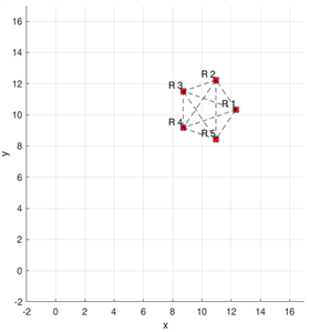
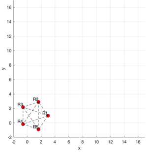
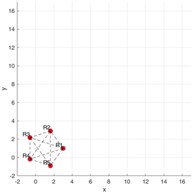
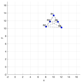
Example 1. Consider 5 robots positioned on a circle with center (1,1) and radius r=2. They navigate from an initial state at (1,1) to a final state at (10,10) while maintaining the desired formation. The initial and final positions are illustrated in Figure 1 and Figure 2, respectively.

tu_pian_25.png

Figure 1. Initial formation

tu_pian_26.png

Figure 2. Final formation

tu_pian_27.png

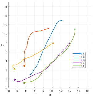
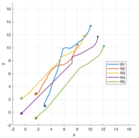
Figure 3. Robot trajectories

The five-robot pentagon moves rigidly toward the goal while preserving its geometry shape, non-intersecting paths verify collision-free motion and near-zero formation error, as shown in Figure 3, where the trajectories of the robots are illustrated.

3.2 Navigation with deformation (scale and rotation)

In practice, it is not feasible to achieve a strictly rigid deformation. Therefore, we introduce a deformation tolerance $\varepsilon^{\text {adapt}}>0$  as follows:

$\left\|\delta_{i j}^{a d a p t}(t)-\Gamma(t) \delta_{i j}^d\right\| \leq \varepsilon^{a d a p t}$      (19)

Remark 4. The deformation matrix $\Gamma(t)$ remains invertible for all $t$. This invertibility ensures that the formation can always be recovered to its original shape whenever external constraints or collision-avoidance manoeuvres no longer apply.

For simplicity, we focus on the two-dimensional setting. However, the same approach can be extended analogously to higher dimensions n≥2 without fundamental change in the methodology.

The deformation matrix is given as:

$\Gamma(t)=s(t) \cdot R(\theta(t))$,    (20)

where, s(t) is a scalar function (the scale factor) that allows the formation to expand or contract in the plane, R(θ(t)) is the rotation matrix given by:

$R(\theta(t))=\left[\begin{array}{cc}\cos (\theta(t)) & -\sin (\theta(t)) \\ \sin (\theta(t)) & \cos (\theta(t))\end{array}\right]$.    (21)

There are numerous ways to specify the time-dependent scale s(t) and rotation θ(t). Two illustrative cases are:

1. Linear Variations:

$s(t)=1+\beta_1 t$ , $\beta_1$ is a small constant rate of expansion or contraction, $\theta(t)=\beta_2 t$, $\beta_2$ is a constant rotational speed.

2. Sigmoidal Variations:

$s(t)=\frac{1}{1+e^{-\beta\left(t-t_0\right)}}$, $\beta>0$, $t_0$ represents the midpoint of the switch, $\theta(t)=\theta_0+\gamma s(t)$, $\theta_0$ is the initial angle of the formation, $\gamma$ is a rotation factor (or rotation gain).

Example 2. Consider 5 robots in an initial state arranged in a circle of radius r=2 with the formation center at (1,1). In this example, a simple deformation (comprising both scaling and rotation) is applied to adjust the formation as the robots navigate toward a final state with the center at (10,10) while maintaining the desired formation, as illustrated in Figure 4 for the initial position and Figure 5 for the final position.

The multi-robot team translates from its initial coordinates to the target location while simultaneously scaling and rotating the formation, maintaining strict inter-agent separation and achieving collision-free trajectories throughout the maneuver, as shown in Figure 6.

tu_pian_28.png

Figure 4. Initial formation

tu_pian_29.png

Figure 5. Final formation

tu_pian_30.png

Figure 6. Robot trajectories

3.3 Navigation with deformation (shape change)

Let Let $\delta_{i j}^{S h_1}$ and $\delta_{i j}^{S h_2}$ denote the desired relative positions between robots i and j corresponding to the shapes Sh₁ and Sh₂, respectively. We introduce a continuous transition function $\beta(t) \in[0,1]$  such that:

• $\beta(0)=0:$ Initially, the formation is Sh₁.
• $\beta(t)=1$  for all for all $t \geq T_{\text {trans}}$: After a certain transition time, the formation becomes Sh₂.

The desired relative offset is defined as:

$\delta_{i j}^d=(1-\beta(t)) \delta_{i j}^{S h_1}+\beta(t) \delta_{i j}^{S h_2}$.  (22)

Remark 5. The following functions can be used like a transition functions:

• $\beta(t)=\min \left\{1, \frac{1}{T_{\text {trans }}}\right\}$.
• $\ \beta(t)= \begin{cases}0 & t \leq t_{\text {start}}, \\ \frac{1}{1+e^{-k\left(t-t_0\right)}} & t_{\text {start }}<t<t_{\text {end}}, \\ 1 & t \geq t_{\text {end}} .\end{cases}$   

where, $k>0$ is a parameter, t₀ is the midpoint (which means that the transition is halfway complete at $t=t_0$, $t_{\text {start}},  \,t_{\text {end}}$ are the start and end transitions, respectively.

The distributed QP problem is solved locally by each robot based on the information from its neighbors:

$\min _{u_i} \frac{1}{2}\left\|u_i-u_{d e s}\right\|^2+\lambda \sum_{j \in \mathcal{N}_i}\left\|p_i-p_j-\delta_{i j}^d\right\|^2$.  (23)

This formulation allows each robot to use local information (via distributed consensus) to adjust its control input and drive the formation from shape Sh₁ to shape Sh₂ over time.

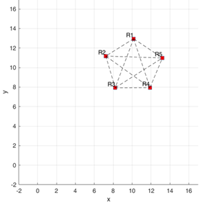
Example 3. Consider 5 robots in an initial state arranged in a circle of radius r=2 with the formation center at (1,1). In this example, the formation transitions from a circle to a triangle while simultaneously navigating toward the target.

tu_pian_31.png

Figure 7. Initial formation

tu_pian_32.png

Figure 8. Final formation

tu_pian_33.png

Figure 9. Robot trajectories

As shown in Figures 7-9, the five-robot team successfully executes a dual objective translation toward the goal and continuous morphing from an initial circular lattice (radius 2 m, center at (1,1)) to a terminal triangular pattern without a single inter-robot collision. The smooth, non-intersecting trajectories confirm that the CBF-QP supervisor enforces the prescribed minimum separations at every instant, even while accommodating the coupled inertial dynamics and the non-convex deformation path. These results underscore the controller’s ability to orchestrate complex, real-time formation reshaping while rigorously maintaining safety guarantees.