Ika Oktavia Suzanti![]() | Husni
| Husni![]() | Rika Yunitarini
| Rika Yunitarini![]() | Andharini Dwi Cahyani
| Andharini Dwi Cahyani![]() | Miswanto*
| Miswanto*![]() | Putu Sugiartawan
| Putu Sugiartawan![]() | Yonathan Ferry Hendrawan
| Yonathan Ferry Hendrawan![]()
© 2025 The authors. This article is published by IIETA and is licensed under the CC BY 4.0 license (http://creativecommons.org/licenses/by/4.0/).
OPEN ACCESS
Text mining is a process of extracting knowledge contained in unstructured text, using Natural Language Processing techniques to analyze, group, and extract patterns. Text mining enables various tasks, such as text classification, information extraction, and sentiment analysis. In this study, a comparison was made between Artificial Neural Network (ANN) and Support Vector Machine (SVM) with hyperparameter tuning in classifying Indonesian tourism news. The classification was divided into 4 classes, namely natural tourism, artificial tourism, cultural tourism, and non-tourism. With the use of hyperparameter tuning on SVM, the highest F1-score was 97.73% and the average computing time was 90.35 seconds. The classification results using ANN produced an F1-score value of 97% and a computing time of 166.87 seconds. This shows that the traditional machine learning methods can match the accuracy of deep learning while requiring less computing time.
text mining, text classification, tourism, SVM, hyperparameter tuning, ANN
Indonesia has extraordinary tourism potential. Various tourist attractions range from enchanting natural attractions to culinary tours that provide typical foods from various regions in Indonesia, which is known as a country rich in spices [1]. This sector makes thousands of information and news available on the Internet, to facilitate the search for a tourist attraction or restaurant to be visited. The development of various tourism websites, social networks, and tourism news, a large amount of data on tourism topics being produced and posted regularly. Many people who plan a trip use this information as a consideration for choosing a destination and interesting places to visit [2-4].
Text mining is the process of extracting knowledge contained in unstructured text. The text mining process used Natural Language Processing (NLP) techniques, machine learning, and statistics, to analyze, group, and extract patterns from text. By using text mining, some works like text classification, information extraction, sentiment analysis and social network analysis can be carried out [5]. NLP techniques are a way to identify communication between humans and machines (computers). If computers can understand natural language, then communication between computers and humans should be able to be done in a language that can be understood by humans [6, 7]. Text classification is also called text categorization [8]. Text classification is part of supervised text mining, which is defined as grouping messy text into the right class based on the content of the text [9]. The accuracy of manual text classification can easily be affected by human factors such as fatigue while using machine learning to automate text classification can provide more reliable and subjective results. So that can help improve efficiency and speed up classification time [10]. In classifying text, it is very important for users to define classification categories and extract related features so that a reliable text classifier model is ultimately built. Classification can be grouped into 2 types: binary and multi-class classification [11]. Binary classification is the grouping of data into one of two classes, namely yes or no, positive or negative, as in the case of sentiment analysis [12-14]. In multi-class classification, the number of existing classification classes results is more than 2 classes [6, 8, 11, 15-17]. While classification with multi-labels is included in the multi-class group, but refers to the number of labels in the case to be resolved can be more than one [11, 18]. Although the majority of text classification is done in English, this work has also been done in several languages, including Indonesian [15], Chinese [19], Arabic [20], Turkish [16], German [21], Spanish [22], and Russian [23]. Automatic text classification is also used in various fields such as industry [24], government [13, 19, 25], news [6, 17, 26], and detecting someone's personality based on social media posts [27].
In classifying text, a document is assumed to be a "bag of words" which is then identified by the class by the selected method through the number of words that appear in the bag. Not infrequently, the use of word rankings is added to determine the most relevant document topics [9]. Several methods, both machine learning and deep learning, are widely used in text classification. In machine learning, these methods include Decision Tree, Random Forest, Naïve Bayes, K-Nearest Neighbor (KNN), and Support Vector Machine (SVM) [11, 12, 15, 16]. SVM is the most widely used machine learning classification method because this method is very good at handling high-dimensional data and is able to overcome data balancing problems [28]. SVM has several types of kernel tricks that can be used to maintain a balance between minimizing errors and maximizing classification margins.
While in deep learning, Artificial Neural Network (ANN), Long Short-Term Memory (LSTM), CNN-LSTM, Bidirectional Encoder Representations from Transformers (BERT) [13, 19, 25, 29, 30]. ANN is a predecessor method or initial form for deep learning, where this method has a simple architecture. The need for computing machine specifications for this method is also lower compared to other deep learning methods [28].
Text classification is a job that is generally divided into 3 stages, namely feature extraction, feature selection, and text classification [8]. Feature selection (FS) in machine learning is a stage of reducing or selecting a number of features so that only relevant features are stored [31]. This feature selection process can reduce the computation time of the model when classifying and recognizing data patterns. By eliminating redundant features, it is expected that accurate data will be obtained so that the accuracy of the model can remain high but the computation time required is reduced [18, 20, 32]. Information gain is the best feature selection method in text processing because it has the advantages of simplicity in implementation [33, 34]. Analysis of Variance (ANOVA) is a statistical method that can be used to determine the probability of membership of data to a certain class compared to other classes. ANOVA is used in feature selection to measure the difference in the probability value of features in a certain class compared to other classes, so that significant feature values are obtained according to the intended class [32].
This work proposes a comparative study of SVM as the best machine learning method and ANN as a precursor to deep learning methods, with ANOVA and Information Gain as feature selection. The goal is to find the best parameter values for multi-class classification with specific Indonesian tourism news data. Comparison of the performance of a combination of several selected parameters is then measured by computing time and effectiveness evaluation value based on the confusion matrix.
Text mining, also known as text data mining, utilizes computer programs and algorithms to mine large amounts of text, such as books, articles, websites, or social media posts, to find valuable and hidden information. This information can be patterns, trends, insights, or specific pieces of knowledge that are not immediately apparent when reading the text. Text mining helps people in large amounts of text data quickly and efficiently, making it easier to find important information for future needs [5].
Text classification is a branch of text mining that specifically performs grouping of messy text data into specific groups based on the content of the text. Basically, the task of text classification is to classify raw text into one or more pre-defined categories [35]. For example, in a sentiment analysis task, text can be categorized as "positive", "negative", or "neutral". In news clustering, an article can be classified into categories such as "politics", "sports", or "entertainment".
In general, text classification can be divided into two types based on the number of categories a document can have:
1. Binary Classification: Where text is classified into one of two classes. A common example is the classification of emails as “spam” or “non-spam”.
2. Multiclass Classification: Where text is classified into more than two classes. For example, in a topic clustering task, text can be classified into multiple topics such as “business”, “health”, “technology”, etc.
2.1 Dataset
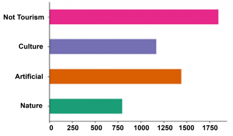
The dataset was obtained by crawling the detik.com website for news articles containing the keyword "tourism" using the Beautiful Soup library in Python. The obtained news spans the period from August 9 to November 20, 2023. There are 5,252 articles containing 2,057,528 words, which are divided into four classes: nature, culture, artificial, and non-tourism. The labeling process is done manually by the authors and then validated by the Bangkalan Culture and Tourism Office.
The statistics of the news data used are shown in Figure 1 where the nature category has 795 articles, the artificial category has 1,441 articles, the culture category has 1,168 articles, and the non-tourism category has 1,845 articles.
Figure 1. Data statistics
2.2 Preprocessing
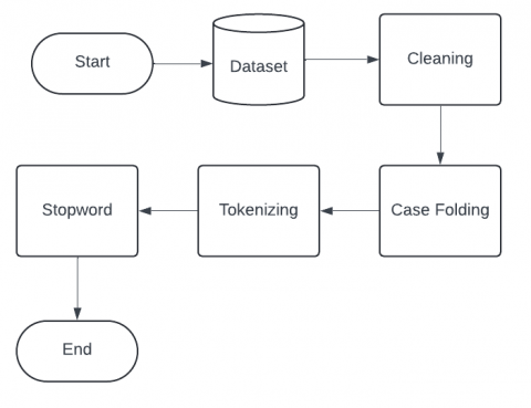
Preprocessing is the first step in processing data that used to clean, organize, and change raw data into a format that is more suitable for analysis or modeling. The preprocessing steps carried out in this study are shown in Figure 2.
Figure 2. Data preprocessing
Cleaning is the process of cleaning characters such as punctuation and symbols. In case of folding, all characters are adjusted to lowercase to avoid inconsistencies in writing. Furthermore, tokenizing is used to extract words from sentences. Stopword Removal is the next step, where common words that are less meaningful are removed to increase the relevance and accuracy of text analysis. Words such as "dan", "atau", "di", which often appear but have no meaning, are considered stopwords and will be removed at this phase. The stopword list used is Indonesian stopwords in NLTK. An example of the results of preprocessing is shown in Table 1.
Table 1. Preprocessing article
|
Sentence |
Cleaning |
Folding Case |
Tokenization |
Stopword Removal |
|
Menelusuri Destinasi Ekowisata Hutan Mangrove di Nusa Lembongan |
Menelusuri Destinasi Ekowisata Hutan Mangrove di Nusa Lembongan |
menelusuri destinasi ekowisata hutan mangrove di nusa lembongan |
['menelusuri', 'destinasi', 'ekowisata', 'hutan', 'mangrove', 'di', 'nusa', 'lembongan'] |
['menelusuri', 'destinasi', 'ekowisata', 'hutan', 'mangrove', 'nusa', 'lembongan'] |
|
Weekend di Jakarta, Bisa Lihat Pameran Wisata dan Budaya Zhejiang |
Weekend di Jakarta Bisa Lihat Pameran Wisata dan Budaya Zhejiang |
weekend di jakarta bisa lihat pameran wisata dan budaya zhejiang |
['weekend', 'di', 'jakarta', 'bisa', 'lihat', 'pameran', 'wisata', 'dan', 'budaya', 'zhejiang'] |
['weekend', 'jakarta', 'lihat', 'pameran', 'wisata', 'budaya', 'zhejiang'] |
|
Jangan Harap Ada Wisata Seperti 'Disneyland' di IKN |
Jangan Harap Ada Wisata Seperti Disneyland di IKN |
jangan harap ada wisata seperti disneyland di ikn |
['jangan', 'harap', 'ada', 'wisata', 'seperti', 'disneyland', 'di', 'ikn'] |
['harap', 'wisata', 'disneyland', 'ikn'] |
2.3 Term Frequency-Inverse Document Frequency (TF-IDF)
TF-IDF is a word weighting used to change data that was originally text into numeric data. If there is a word has a high TF-IDF value, it can be interpreted that it is frequently appears in the document being analyzed [17]. In the process of giving weights using the TF-IDF method, the initial step is to calculate the TF value by evaluating how often a word appears in a document. In Eq. (1) is a function to calculate the TF value in a document.
${{\text{W}}_{\text{i},\text{d}}}=\left\{ \begin{matrix} 1+log10\text{t}{{\text{f}}_{\text{i},\text{d}}},\text{ }\!\!~\!\!\text{ if }\!\!~\!\!\text{ t}{{\text{f}}_{\text{i},\text{d}}}>0 \\ 0,\text{ }\!\!~\!\!\text{ if }\!\!~\!\!\text{ t}{{\text{f}}_{\text{i},\text{d}}}=0 \\ \end{matrix} \right.$ (1)
where, Wi,d = score for word “” in article “d”; tfi,d = frequency of occurrence of word “t” in article “d”.
If the word “i” appears at least once in document “d”, then the tf score is calculated by taking the base 10 logarithm of the word's frequency of occurrence and adding 1 to the result. However, if the word “t” does not appear at all in the document, then the TF score is 0. After calculating the TF value using the formula mentioned above, the next step is to calculate the IDF value. IDF takes into account several important words in each set of documents. Eq. (2) is a function for calculating the IDF value in a document.
$\text{IDF}\left( \text{i},\text{D} \right)=\text{lo}{{\text{g}}_{10}}\left( \frac{\text{N}}{\text{DF}\left( \text{i},\text{D} \right)} \right)$ (2)
where, IDF (i,D) = IDF score for word "i" in total article (D); N = total article; "DF" (i,D) = amount of article in total (D) contains the word "i".
After getting the TF and IDF values, we can multiply them together to get the TF-IDF score with Eq. (3).
$\text{TF}-\text{IDF}\left( \text{t},\text{d},\text{D} \right)=\text{TF}\left( \text{t},\text{d} \right)\times \text{IDF}\left( \text{t},\text{D} \right)$ (3)
With Eqs. (1)-(3), the TF-IDF score can be calculated for each word in each article used (D). This score provides a weight that indicates how important a word is in to entire article collection. The higher the TF-IDF value, means more important the word is in that article and the collection as a whole.
2.4 Feature selection
In the text classification, FS refers to process of choosing most important and relevant features, such as words, phrases, n-grams, or other characteristics, from a dataset that contributes to distinguishing between different classes.
(1) Information Gain (IG)
The IG is one of FS methods to measure how much information a feature provides about the target class. IG is usually used in FS method in text processing because it has the advantages of simplicity in implementation [33, 34]. It shows the dependency between the feature and the target class. Eq. (4) is a general equation used in IG.
$\text{IG}\left( \text{X},\text{Y} \right)=\underset{\text{x}\in \text{X}}{\mathop \sum }\,\underset{\text{y}\in \text{Y}}{\mathop \sum }\,\text{P}\left( \text{x},\text{y} \right)\text{log}\left( \frac{\text{P}\left( \text{x},\text{y} \right)}{\text{P}\left( \text{x} \right)\text{P}\left( \text{y} \right)} \right)$ (4)
where, P(x,y) is the joint probability of x and y. P(x) and P(y) are the marginal probabilities of x and y.
This feature selection is widely used in text classification to select the most informative features about the target class [34].
(2) ANOVA
ANOVA is a statistical method used to compare the averages of two or more data groups. ANOVA can be used to test the differences between the groups [36]. In the feature selection process, ANOVA works by selecting features that have a significant average difference value and have been below a predetermined threshold [32]. ANOVA is one of the feature selection methods applied with the aim of measuring the difference between feature values based on a certain class so as to obtain significant features. In feature selection with ANOVA, data is obtained from the TF-IDF results. After being obtained, the average calculation process is carried out for each group (Eq. (5)) then the overall average of all groups is calculated (Eq. (6)). Furthermore, the calculation of the variance between groups (Eq. (7)) and the variance within the group (Eq. (8)) is carried out. After that, the F1-score value is calculated from the variance between groups divided by the variance within the group. The F value taken is the one that is smaller than the predetermined threshold limit so that relevant features are obtained. The ANOVA function is defined in Eqs. (5)-(9) [36].
$\left[ \overline{{{\text{X}}_{\text{grand }\!\!~\!\!\text{ }}}}=\frac{\mathop{\sum }_{\text{i}=1}^{\text{k}}\quad {{\text{n}}_{\text{i}}}{{{{\bar{X}}}}_{\text{l}}}}{\text{N}} \right]$ (5)
where, $\overline{{{\text{X}}_{\text{i}}}}\text{ }\!\!~\!\!\text{ }$is the average of the -th group (i). ${{\text{X}}_{\text{ij}}}\text{ }\!\!~\!\!\text{ }$is the observation value in the -th group (i), the -th observation (j). ${{\text{n}}_{\text{i}}}~$is the number of observations in the -th group (i).
$\left[ \text{SST}=\underset{\text{i}=1}{\overset{\text{k}}{\mathop \sum }}\,\underset{\text{j}=1}{\overset{{{\text{n}}_{\text{i}}}}{\mathop \sum }}\,{{\left( {{\text{X}}_{\text{ij}}}-\overline{{{\text{X}}_{\text{grand }\!\!~\!\!\text{ }}}} \right)}^{2}} \right]$ (6)
where, SST measures the total variation in the data. $\overline{{{\text{X}}_{\text{grand}}}}$ is the total average of all data. ${{\text{X}}_{\text{ij}}}$ is the observation value in the th group (i), the th observation (j).
$\left[ \text{SSB}=\underset{\text{i}=1}{\overset{\text{k}}{\mathop \sum }}\,{{\text{n}}_{\text{i}}}{{\left( {{{{\bar{X}}}}_{1}}-\overline{{{\text{X}}_{\text{grand }\!\!~\!\!\text{ }}}} \right)}^{2}} \right]$ (7)
where, SSB measures variation between groups. $\overline{{{\text{X}}_{\text{i}}}}$ is the average of the -th group (i).
$\left[ \text{SSW}=\underset{\text{i}=1}{\overset{\text{k}}{\mathop \sum }}\,\underset{\text{j}=1}{\overset{{{\text{n}}_{\text{i}}}}{\mathop \sum }}\,{{\left( {{\text{x}}_{\text{ij}}}-{{{{\bar{X}}}}_{1}} \right)}^{2}} \right]$ (8)
where, SSW measures variation within groups. ${{\text{X}}_{\text{ij}}}$ is the observation value in the -th group (i), the -th observation (j). $\overline{{{\text{X}}_{\text{i}}}}$ is the average of the -th group (i).
$\left[ F=\frac{SSB}{SSW} \right]$ (9)
2.5 SVM
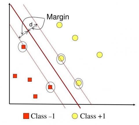
SVM is a machine learning algorithm that is used for regression or classification [37]. In principle, SVM is used for binary classification tasks, which separate two classes. There are various options in selecting the separator plane, as shown in Figure 3, which can separate all data based on each class. However, not all problems can be solved with a linear approach. Some problems may have complex decision boundaries and cannot be perfectly separated using straight lines.
Figure 3. Linear SVM
For multiclass classification, the principle used is the same as the general linear SVM classification. There are 2 approaches commonly used in multiclass classification, namely [38]:
One additional approach to address these challenges is to apply the Kernel Trick. Kernel Trick is a kernel trick in SVM that allows data to be extracted more concisely without requiring detailed analysis of the underlying coordinates. By using kernel functions, SVM can work effectively in higher-dimensional spaces and address problems that cannot be solved linearly. In the context of multiclass classification, kernel functions play a crucial role in supporting SVM in formulating models that are able to represent more complex relationships between features and class labels. Several types of kernel functions that can be applied to multiclass classification are shown in Eqs. (10)-(13).
(i) Kernel polynomial
In SVM, a polynomial kernel is used when the data cannot be linearly selected. In addition, the polynomial kernel is also effective in handling classification problems on normalized training datasets, as explained by Eq. (10) [39].
$K\left( x,y \right)={{(x\cdot y+c)}^{d}}$ (10)
where, x and y are two input vectors. c is the bias parameter. d is the degree of the polynomial, which is a tunable parameter.
(ii) RBF kernel
The RBF kernel, often known as the Gaussian kernel, is a type of kernel function used in SVM to approximate two data points in a given parameter space [40]. The equation for the RBF kernel is shown in Eq. (11).
$K\left( {{x}_{i}},{{x}_{j}} \right)=\text{exp}\left( -\frac{{{\left| {{x}_{i}}-{{x}_{j}} \right|}^{2}}}{2{{\sigma }^{2}}} \right)$ (11)
where, xi and xj are two data vectors in feature space. $|{{x}_{i}}-{{x}_{j}}{{|}^{2}}$ is the square of the distance between xi$~$and xj.
$\sigma $ is a parameter referred to as the kernel width. $\sigma $ smaller values will produce a sharper kernel, while $\sigma ~$larger values will produce a wider kernel.
(iii) Linear kernel
The linear kernel function is a method for measuring the similarity between two feature vectors. The linear kernel function gives a value that reflects the extent to which two samples are similar: the higher the value, the more similar the two samples are. The linear kernel function is defined by Eq. (12).
$K\left( {{x}_{i}},{{x}_{j}} \right)=x_{i}^{T}\cdot {{x}_{j}}$ (12)
where, K represents the linear kernel function; xiand xj feature vector of the two samples to be compared; T shows the transpose operation.
2.6 ANN
ANN is a computational method that works in a way that resembles the human biological nervous system, which is able to learn from available data and produce the desired output by adjusting previously existing information [23]. In the ANN method, there are many terms, namely, weight, layer, neuron, input, output, and hidden layers [24].
Each layer has neurons, and these neurons are connected to signals; the signals will be given weight at the beginning of the process. Weight is a measure of the relationship between neurons to each other. This is used in an attempt to move data from one layer to another [24]. An illustration of how ANN works is shown in Figure 4, where x = input layer, y = hidden layer, z = output layer, and w = weight. In ANN model, there are several activation functions. In this study, the activation function used in the hidden layer is the ReLu activation function, and the output layer uses the Softmax activation function.
Figure 4. ANN architecture
ReLu function is a non-linear function where the activation of neurons is not done simultaneously, and only when the output of the linear transformation is zero [30]. The ReLu activation function uses Eq. (13), which is specifically used in artificial neural networks to learn complex patterns in data.
$f\left( x \right)=max\left( 0,x \right)$ (13)
The Softmax activation function has the advantage of producing output probability values ranging from 0-1 and the total probability is equal to 1. The Softmax function in multi-class classification will calculate the probability value for each class and will provide a high probability for the target class. The Softmax activation function formula is shown in Eq. (14).
$\text{Softmax}\left( {{x}_{i}} \right)=\frac{{{e}^{{{x}_{i}}}}}{\mathop{\sum }_{j=1}^{n}{{e}^{{{x}_{j}}}}}$ (14)
2.7 Evaluation
In modeling the classification process, it is necessary to evaluate the performance of the system to measure how good the method is used [41]. The commonly used method in evaluating a system is confusion matrix. A confusion matrix is a method of evaluating the level of accuracy, precision, recall, and F1-score from the algorithm used to classify the data [31]. The confusion matrix table in this study is shown in Table 2.
Table 2. Confusion matrix
|
Prediction |
Actual |
|||
|
A |
B |
C |
D |
|
|
A |
TN |
FN |
TN |
TN |
|
B |
FP |
TP |
FP |
FP |
|
C |
TN |
FN |
TN |
TN |
|
D |
TN |
FN |
TN |
TN |
The detailed explanation of Table 2 is:
True Positive (TP): numbers of data that actual and predicted value are the same (both predicted as class B).
True Negative (TN): number of data that is actually not class B and predicted not to be class B.
False Negative (FN): number of data that is actually class B but is predicted not to be class B.
False Positive (FP): number of data that are actually not class B but are predicted to be class B.
Accuracy is a measurement to determine model performance in classifying into the correct class with the following formula:
$\text{Accuracy}=\frac{\text{TP}+\text{TN}}{\text{TP}+\text{TN}+\text{FP}+\text{FN}}$ (15)
Precision is percentage of right class B predictions divided by class B predictions, with the following formula:
$\text{Precision}=\frac{\text{TP}}{\text{TP}+\text{FP}}\times 100\text{ }\!\!%\!\!\text{ }$ (16)
Recall is percentage of right class B predictions divided by class B actual number, with the following formula:
$\text{Recall}=\frac{\text{TN}}{\text{TN}+\text{FN}}\times 100\text{ }\!\!%\!\!\text{ }$ (17)
F1-score is measuring the balance between recall and precision. F1-score range values is between 0-1.
F1-score$=2\times \frac{\text{Recall}\times \text{Precision}}{\text{Recall}+\text{Precision}}\times 100\text{ }\!\!%\!\!\text{ }$ (18)
In the evaluation value of multiclass classification, the calculation of precision and recall is slightly different from binary classification. In this study, the SVM classification approach used is One versus All or OvA, therefore the calculation of recall and precision uses the micro-averaging approach. This approach calculates the recall and precision values of each class separately for each class so that a confusion matrix is obtained similar to binary classification [38].
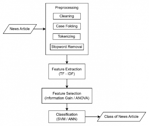
3.1 Data analysis
Figure 5 shows an overview of the sequence of steps performed on the system. The first step begins with preprocessing the news article. In the preprocessing stage, cleaning, case folding, tokenizing, and stopword removal are carried out. After preprocessing, feature extraction is carried out using TF-IDF. At this stage, the data is given a value or weight according to the number of occurrences of the word in the article. Feature selection is then carried out using the IG or ANOVA method. The division of training data and testing data is carried out using K-fold cross validation with a value of K = 10. Furthermore, classification is carried out using SVM or ANN. When using the SVM method, hyperparameter tuning is previously carried out using the Grid Search method to find the most optimal combination of hyperparameters that will be used by the SVM model. The hyperparameters that were changed include C, gamma, and kernel type. The classification results will then be measured for precision, recall, accuracy, F1-score and the computation time required.
Figure 5. System flowchart
The news articles used were obtained from crawling using BeautifulSoup with keywords “pariwisata” on the Detik.com page with a news publication period ranging from August 9 to November 20, 2023, in the tourism news category of 5,252 articles with a total of 2,057,528 words and labeled into 4 classes, namely nature, culture, artificial and not tourism news. Data labeling is done manually and validated by the Bangkalan Culture and Tourism Office.
Table 3. Word distribution
|
Category |
Number of Documents |
Word Count |
|
Natural |
795 |
318,514 |
|
Artificial |
1,441 |
533,772 |
|
Culture |
1.168 |
488,510 |
|
Not Tourism |
1,845 |
716,732 |
The statistics of the news data used are shown in Table 3 where the nature category has 795 documents with a word count of 318,514, the artificial category has 1,441 documents with a word count of 533,772, the culture category has 1,168 documents with a word count of 488,510, and the non-tourism category has 1,845 documents with a word count of 716,732. Further analysis of the number of words in each news as seen in Table 4. The word distribution table shows the variation in the number of words in the news to be classified. From Table 4, it can be seen that the least number of words is 103, which is found in the 1683rd news, while the greatest number of words is 1893, which is found in the 3923rd news.
Table 4. Detail word distribution
|
Document |
Word Count |
|
D1 |
583 |
|
D2 |
424 |
|
D3 |
360 |
|
…. |
… |
|
D5251 |
580 |
|
D5252 |
720 |
Wordcloud is used to get an overview of the words that appear from each category. Figure 6 is a wordcloud of 4 categories in the classification of tourism news created in this study. Word size describes the frequency of word occurrence in all articles in each category.
Figure 6. Wordcloud for each category
3.2 Classification using SVM
At this stage, hyperparameter tuning is carried out to find the most optimal parameter values in the SVM method using grid search with hyperparameter values C = [0.1, 1, 10, 100, 1000], gamma = [0.001, 0.01, 0.1, 1, 10], kernel = [linear, polynomial, rbf], the multiclass approach used is OvA in the scikit-learn library. The threshold value used in the selection of IG and ANOVA features is 5% [34], and Stratified K-Fold 10. The K-Fold used is also stratified K-Fold because the processed data is unbalanced. By using stratified K-Fold, the percentage distribution of data for each fold will be balanced according to the percentage of the overall data.
The highest evaluation value results are obtained at a value of C = 1, Gamma = 10, polynomial kernel as shown in the Table 5.
Table 5. SVM result
|
Scenario |
Accuracy |
Precision |
Recall |
F1-Score |
Time (s) |
|
NO FS |
97.72% |
97.84% |
97.72% |
97.73% |
87.13 |
|
IG |
97.72% |
97.82% |
97.72% |
97.72% |
82.6 |
|
ANOVA |
97.72% |
97.79% |
97.72% |
97.71% |
61.88 |
Based on Table 5, it can be concluded that the accuracy, precision, recall and F1-score values are not too significant in the 3 scenarios. However, compared to the use of IG feature selection, ANOVA can reduce the computation time by up to 26 seconds faster. While in FS with IG, the computation time is only reduced by about 5 seconds.
This is because the complexity of ANOVA calculations is simpler than IG. Calculations in ANOVA are only basic statistical operations such as addition, multiplication or division, while in IG using logarithmic calculations with looping to calculate the entropy value of all features. This is also what makes even though the number of features processed is less than without feature selection, the computing time is not significantly reduced.
3.3 Classification using ANN
Classification with ANN was performed with parameters of batch size 526, learning rate 0.001, 2 hidden layers, Adam optimizer, ReLu optimization function on the hidden layer, Softmax activation function on the output layer, and the number of epochs is 10. To maintain the same reproducibility results even though the model is run repeatedly, the random seed value is set to 42.
Table 6. ANN result
|
Scenario |
Accuracy |
Precision |
Recall |
F1-Score |
Time (s) |
|
NO FS |
97.34% |
97% |
98% |
97% |
166.87 |
|
With FS |
96.77% |
97% |
97% |
97% |
78.7 |
The results of classification with ANN, the use of FS has a significant effect on reducing computing time by up to 50% compared to not using FS, as shown in Table 6. This shows that the use of machine learning can match the accuracy of deep learning with faster computing time.
The significant difference in computation time between ANN and SVM occurs because the model architecture and parameters used in the SVM classification process are fewer and not as complex as in the ANN architecture. The effect of the number of epochs is also a factor in the ANN computation time being longer because the more epochs, the more time the model needs to repeat the learning.
The use of FS in classification process is to reduce the number of features processed by the model. With FS, features that do not have significant importance values can be removed so that in the end, features processed by model are truly important features. In the end, although the main purpose of using FS is to reduce computing time, in certain cases, such as in ANN, the use of FS can also reduce accuracy because this process does not pay attention to the relationship or attention of each word.
In this study, a comparison was made between text classification models with SVM and ANN based on their time and performance. Both models also used scenarios with and without the use of feature selection.
With the use of hyperparameter tuning on SVM in the parameters C, gamma, and the type of kernel used, it shows that the polynomial kernel has the highest F1-score value of 97.73% and the average computation time is 90.35 seconds. In the RBF kernel, the highest F1-score value is 96.19% with an average computing time of 117.26 seconds. While in the linear kernel, the F1-score value decreases by 4.2% to 93.53% but the computing time is shorter at 86.68 seconds. The use of IG feature selection managed to reduce the time by 10 seconds to 80.69 seconds while maintaining the F1-score value of 97.72%. While the use of ANOVA feature selection, while maintaining the F1-score of 97.71% was able to reduce the average computing time to 71.87 seconds. This computing time is up to 20 seconds faster than without the use of feature selection. The classification results using ANN with a learning rate of 0.001, 2 hidden layers, Adam optimizer, ReLu optimization function on the hidden layer, Softmax activation function on the output layer, and the number of epochs 10 produced an F1-score value of 97% and a computation time of 166.87 seconds. The use of feature selection managed to reduce the computation time by 20 seconds.
The limitation of this study is that the dataset used only comes from specific news websites, so that comparison with existing datasets that are already available can be used as exploration material for the proposed parameter combinations.
In future works, comparisons can be made with more recent baseline machine learning or deep learning methods, such as BERT or derivatives of ANN, such as LSTM. In further research, the use of embedding features compared to TF-IDF can capture information that is more appropriate to the specified class.
[1] Husain, Triwijoyo, B.K., Taufik, M., Mawengkang, H. (2024). Optimization model of multi criteria decision analysis for smart and sustainable sport tourism planning development problem. Mathematical Modelling of Engineering Problems, 11(11): 3035-3046. https://doi.org/10.18280/mmep.111116
[2] Abbasi-Moud, Z., Vahdat-Nejad, H., Sadri, J. (2021). Tourism recommendation system based on semantic clustering and sentiment analysis. Expert Systems with Applications, 167: 114324. https://doi.org/10.1016/j.eswa.2020.114324
[3] Hayashi, T., Yoshida, T. (2018). Development of a tour recommendation system using online customer reviews. In International Conference on Management Science and Engineering Management, pp. 1145-1153. https://doi.org/10.1007/978-3-319-93351-1_90
[4] Renjith, S., Sreekumar, A., Jathavedan, M. (2020). An extensive study on the evolution of context-aware personalized travel recommender systems. Information Processing & Management, 57(1): 102078. https://doi.org/10.1016/j.ipm.2019.102078
[5] Jo, T. (2019). Text mining. Studies in Big Data, 45: 1-373. https://doi.org/10.1007/978-3-319-91815-0
[6] Jin, G. (2022). Application optimization of NLP system under deep learning technology in text semantics and text classification. In 2022 International Conference on Education, Network and Information Technology (ICENIT), Liverpool, United Kingdom, pp. 279-283. https://doi.org/10.1109/ICENIT57306.2022.00068
[7] Jearanaitanakij, K., Srithongdee, C., Ketkham, S., Ardsana, O., Kullawan, T., Yongpiyakul, C. (2024). Thai question-answering system using similarity search and LLM. ECTI Transactions on Computer and Information Technology (ECTI-CIT), 18(3): 406-416. https://doi.org/10.37936/ecti-cit.2024183.256043
[8] Cekik, R. (2024). A new filter feature selection method for text classification. IEEE Access, 12: 139316-139335. https://doi.org/10.1109/ACCESS.2024.3468001
[9] Wachsmuth, H., Wachsmuth, H. (2015). Text Analysis Pipelines. Springer International Publishing, pp. 19-53. https://doi.org/10.1007/978-3-319-25741-9
[10] Setiani, E., Ce, W. (2018). Text classification services using naïve bayes for Bahasa Indonesia. In 2018 International Conference on Information Management and Technology (ICIMTech), Jakarta, Indonesia, pp. 361-366. https://doi.org/10.1109/ICIMTech.2018.8528258
[11] Morales-Hernández, R.C., Jagüey, J.G., Becerra-Alonso, D. (2022). A comparison of multi-label text classification models in research articles labeled with sustainable development goals. IEEE Access, 10: 123534-123548. https://doi.org/10.1109/ACCESS.2022.3223094
[12] Madyatmadja, E.D., Yahya, B.N., Wijaya, C. (2022). Contextual text analytics framework for citizen report classification: A case study using the Indonesian language. IEEE Access, 10: 31432-31444. https://doi.org/10.1109/ACCESS.2022.3158940
[13] Yu, B., Deng, C., Bu, L. (2022). Policy text classification algorithm based on BERT. In 2022 11th International Conference of Information and Communication Technology (ICTech), Wuhan, China, pp. 488-491. https://doi.org/10.1109/ICTech55460.2022.00103
[14] Wang, Z., Zhang, Z. (2022). Research convey on text classification method based on deep learning. In 2022 7th International Conference on Intelligent Computing and Signal Processing (ICSP), Xi'an, China, pp. 285-288. https://doi.org/10.1109/ICSP54964.2022.9778518
[15] Amalia, A., Sitompul, O.S., Nababan, E.B., Mantoro, T. (2020). An efficient text classification using Fasttext for Bahasa Indonesia documents classification. In 2020 International Conference on Data Science, Artificial Intelligence, and Business Analytics (DATABIA), Medan, Indonesia, pp. 69-75. https://doi.org/10.1109/DATABIA50434.2020.9190447
[16] Gürcan, F. (2018). Multi-class classification of Turkish texts with machine learning algorithms. In 2018 2nd International Symposium on Multidisciplinary Studies and Innovative Technologies (ISMSIT), Ankara, Turkey, pp. 1-5. https://doi.org/10.1109/ISMSIT.2018.8567307
[17] Lan, M., Tan, C.L., Su, J., Lu, Y. (2008). Supervised and traditional term weighting methods for automatic text categorization. IEEE Transactions on Pattern Analysis and Machine Intelligence, 31(4): 721-735. https://doi.org/10.1109/TPAMI.2008.110
[18] Miri, M., Dowlatshahi, M.B., Hashemi, A. (2022). Evaluation multi label feature selection for text classification using weighted Borda count approach. In 2022 9th Iranian Joint Congress on Fuzzy and Intelligent Systems (CFIS), Bam, Iran, pp. 1-6. https://doi.org/10.1109/CFIS54774.2022.9756467
[19] Liu, S., Tao, H., Feng, S. (2019). Text classification research based on Bert model and Bayesian network. In 2019 Chinese Automation Congress (CAC), Hangzhou, China, pp. 5842-5846. https://doi.org/10.1109/CAC48633.2019.8996183
[20] Hijazi, M.M., Zeki, A., Ismail, A. (2021). Arabic text classification: A review study on feature selection methods. In 2021 22nd International Arab Conference on Information Technology (ACIT), Muscat, Oman, pp. 1-6. https://doi.org/10.1109/ACIT53391.2021.9677185
[21] Scharkow, M. (2013). Thematic content analysis using supervised machine learning: An empirical evaluation using German online news. Quality & Quantity, 47: 761-773. https://doi.org/10.1007/s11135-011-9545-7
[22] del Pilar Salas-Zárate, M., Paredes-Valverde, M.A., Limon, J., Tlapa, D.A., Báez, Y.A. (2016). Sentiment classification of Spanish reviews: An approach based on feature selection and machine learning methods. Journal of Universal Computer Science, 22(5): 691-708. https://doi.org/10.3217/jucs-022-05-0691
[23] Tomin, E., Solnyshkina, M., Gafiyatova, E., Galiakhmetova, A. (2023). Automatic text classification as relevance measure for Russian school physics texts. In 2023 IEEE 16th International Symposium on Embedded Multicore/Many-core Systems-on-Chip (MCSoC), Singapore, pp. 366-370. https://doi.org/10.1109/MCSoC60832.2023.00061
[24] Young, J.C., Rusli, A. (2020). A comparison of supervised text classification and resampling techniques for user feedback in Bahasa Indonesia. In 2020 Fifth International Conference on Informatics and Computing (ICIC), Gorontalo, Indonesia, pp. 1-6. https://doi.org/10.1109/ICIC50835.2020.9288588
[25] Hidayati, N.N., Shaleha, S. (2024). BERTopic analysis of Indonesian biodiversity policy on social media. ECTI Transactions on Computer and Information Technology (ECTI-CIT), 18(3): 260-271. https://doi.org/10.37936/ecti-cit.2024173.255058
[26] Rohman, M.A., Khairani, D., Hulliyah, K., Riswandi, P., Lakoni, I. (2021). Systematic literature review on methods used in classification and fake news detection in Indonesian. In 2021 9th International Conference on Cyber and IT Service Management (CITSM), Bengkulu, Indonesia, pp. 1-4. https://doi.org/10.1109/CITSM52892.2021.9589004
[27] Pratama, B.Y., Sarno, R. (2015). Personality classification based on Twitter text using Naive Bayes, KNN and SVM. In 2015 International Conference on Data and Software Engineering (ICoDSE), Yogyakarta, Indonesia, pp. 170-174. https://doi.org/10.1109/ICODSE.2015.7436992
[28] Li, Q., Peng, H., Li, J., Xia, C., et al. (2022). A survey on text classification: From traditional to deep learning. ACM Transactions on Intelligent Systems and Technology (TIST), 13(2): 1-41. https://doi.org/10.1145/3495162
[29] Wu, Y., Wan, J. (2024). A survey of text classification based on pre-trained language model. Neurocomputing, 616: 128921. https://doi.org/10.1016/j.neucom.2024.128921
[30] Su, X., Song, H., Wang, Y., Wang, M. (2022). A short text topic classification method based on feature expansion and bi-directional neural network. In 2022 International Conference on Artificial Intelligence, Information Processing and Cloud Computing (AIIPCC), Kunming, China, pp. 393-397. https://doi.org/10.1109/AIIPCC57291.2022.00089
[31] Chen, R.C., Dewi, C., Huang, S.W., Caraka, R.E. (2020). Selecting critical features for data classification based on machine learning methods. Journal of Big Data, 7(1): 52. https://doi.org/10.1186/s40537-020-00327-4
[32] Moorthy, U., Gandhi, U.D. (2021). A novel optimal feature selection technique for medical data classification using ANOVA based whale optimization. Journal of Ambient Intelligence and Humanized Computing, 12: 3527-3538. https://doi.org/10.1007/s12652-020-02592-w
[33] Abdul-Rahman, S., Mutalib, S., Khanafi, N.A., Ali, A.M. (2013). Exploring feature selection and support vector machine in text categorization. In 2013 IEEE 16th International Conference on Computational Science and Engineering, Sydney, NSW, Australia, pp. 1101-1104. https://doi.org/10.1109/CSE.2013.160
[34] Jović, A., Brkić, K., Bogunović, N. (2015). A review of feature selection methods with applications. In 2015 38th International Convention on Information and Communication Technology, Electronics and Microelectronics (MIPRO), Opatija, Croatia, pp. 1200-1205. https://doi.org/10.1109/MIPRO.2015.7160458
[35] Naradhipa, A.R., Purwarianti, A. (2012). Sentiment classification for Indonesian message in social media. In 2012 International Conference on Cloud Computing and Social Networking (ICCCSN), Bandung, Indonesia, pp. 1-5. https://doi.org/10.1109/ICCCSN.2012.6215730
[36] Henson, R.N. (2015). Analysis of variance (ANOVA). Brain Mapping, 1: 477-481. https://doi.org/10.1016/B978-0-12-397025-1.00319-5
[37] Rochman, E.M.S., Miswanto, Suprajitno, H., Rachmad, A., Mula’ab, Santosa, I. (2023). Utilizing LSTM and K-NN for anatomical localization of tuberculosis: A solution for incomplete data. Mathematical Modelling of Engineering Problems, 10(4): 1114-1124. https://doi.org/10.18280/mmep.100403
[38] Hsu, C.W., Lin, C.J. (2002). A comparison of methods for multiclass support vector machines. IEEE transactions on Neural Networks, 13(2): 415-425. https://doi.org/10.1109/72.991427
[39] Vinge, R., McKelvey, T. (2019). Understanding support vector machines with polynomial kernels. In 2019 27th European Signal Processing Conference (EUSIPCO), A Coruna, Spain, pp. 1-5. https://doi.org/10.23919/EUSIPCO.2019.8903042
[40] Wang, J., Chen, Q., Chen, Y. (2004). RBF kernel based support vector machine with universal approximation and its application. In International Symposium on Neural Networks, Berlin, Heidelberg, pp. 512-517. https://doi.org/10.1007/978-3-540-28647-9_85
[41] Mehdiyev, N., Enke, D., Fettke, P., Loos, P. (2016). Evaluating forecasting methods by considering different accuracy measures. Procedia Computer Science, 95: 264-271. https://doi.org/10.1016/j.procs.2016.09.332