Ngoc-Hoi Le![]() | Dinh-Chung Dang
| Dinh-Chung Dang![]() | Thi-Anh-Vu Phung
| Thi-Anh-Vu Phung![]() | Thi-Thanh-Nga Nguyen*
| Thi-Thanh-Nga Nguyen*![]()
© 2025 The authors. This article is published by IIETA and is licensed under the CC BY 4.0 license (http://creativecommons.org/licenses/by/4.0/).
OPEN ACCESS
A new model order reduction (MOR) algorithm is presented in the paper. By using the dominance index according to the $H \infty$-norm, to evaluate the contribution of the poles to the output response of the system, the algorithm determines the important poles of the original system that need to be retained in the reduced-order system. The algorithm rearranges the poles on the main diagonal of matrix A so that the important poles are located at the leading positions of the main diagonal. Through the truncation technique, the less important poles will be eliminated and the reduced order system will have only the dominant poles. This algorithm is applied to simplify the 5th order robust controller (the original controller). Comparison and evaluation of the transient response and frequency response of the low-order controller and the fifth-order controller identify some controllers that can replace it. The determination of the most suitable controller to replace the original controller is determined through comparison and evaluation of the control system response. The simulation results have demonstrated the correctness and applicability of this algorithm to the problem of the controller order reduction.
$H \infty$-norm, dominant pole, the main diagonal of matrix, model order reduction algorithm
The balanced truncation algorithm (BTA) was proposed by Moore in his research [1]. The algorithm is divided into two steps: The first step is to determine the transition matrix T and then use it to convert the system to an equivalent equilibrium state. When the system is in this state, the observed Gramian matrix is equal to the control Gramian matrix and has a diagonal form. The next step is to perform the truncation technique with the balanced equivalent system, that is, to delete the rows and columns of the balanced equivalent system. The system obtained after performing the truncation technique is the required order reduction system. Since Moore's initial research [1], many algorithms have been proposed in different directions based on the BTA [1-12], as well as applied to many different problems [13-19].
The BTA is further developed in study [2], and the relationship with Hankel norms is determined in studies [3, 4]. In study [5], the Gramians as well as the Hankel values of the original system were generalized and their importance in the process of performing order reduction according to the balanced truncation algorithm was shown. Stykel [6] proposed the use of equilibrium truncation method for semi-discrete Stroke equation and demonstrated the correctness of the proposed method. In the study [7], the extended Gramian concept was proposed and used to determine the formula for calculating the order-reducing error and to prove the stability preservation of the BTA. The BTA using the extended Gramian concept was also constructed and demonstrated its correctness through illustrative examples.
The stochastic equilibrium truncation method was used for stochastic systems in studies [2, 8, 9] and was generalized and proved to have an error bound in study [10]. According to the stochastic equilibrium truncation method, to determine the Gramians, it is necessary to solve one Lyapunov equation and one Ricati equation. Another equilibrium truncation method is the positive real equilibrium truncation method [9] which is built to reduce the order for positive real passive systems, this method requires solving two Ricati equations when determining two Gramians. For bounded real systems, we can apply the bounded real equilibrium truncation method, this method also requires solving two Ricati equations [11]. When designing the order reduction controller, we can apply the LQG equilibrium truncation method [12], which is considered as the first closed-loop equilibrium method. In the study [13], a scheme for designing a reduced model for continuous T-S fuzzy systems with noise in the FF domain was proposed and the effectiveness of the proposal was demonstrated through a simulation example. In the study [14], it is proposed to use a whole vehicle suspension system model that has been reduced to the minimum step by the minimum step reduction technique, the selection of the minimum step is done through evaluating the response of the original system and the reduced step system. In the study [15], the method of eliminating less important states was applied to determine the reduced-order models of the electronic wedge brake (EWB) model.
In the research [16], through the design problem of controlling the angle of attack of FOXTROT aircraft, the author has built a 6th order optimal controller. By applying the balanced chopping algorithm, the author obtained the 4th order reduced model of the original controller. In the study [17], the authors applied three different order reduction methods to determine the low-order controller to replace the controller of the FOXTROT aircraft angle-of-attack control system. The fourth-order reduced controller was also determined to be the most suitable low-order controller to replace the original controller. Dehkordi and Aghdam [18] proposed to use balanced truncation algorithm to determine low-order IRR filter instead of high-order IRR filter model. The paper results show that balanced truncation algorithm is very effective for high-order IIR systems, where Gramians may not be easily computed for direct order reduction. Hai [19] proposed using the LGQ balanced truncation algorithm to simplify the 30th order IRR filter model and select a 3rd order filter while still ensuring the filter quality.
However, the BTA and algorithms based on this algorithm all use the Hankel singular value as the basis for determining the order-reduced system (with the criterion of eliminating states with small Hankel singular values) without caring about preserving the poles of the original system.
With the approach of preserving the important poles of the original system, many algorithms have been proposed [8, 20-25], this group of algorithms is also called modal truncation. The basic feature of the algorithms belonging to the group of methods preserving the important poles is to help maintain the stability of the reduced-order system when the original system is stable. However, the most fundamental problem of this group of methods is how to choose the important poles? Aoki [20] proposed that the poles that contribute the most to the total output pulse response energy are the important poles. In the study [21], it is proposed to use unit pulses to determine the influence of each pole of the original system, the poles with the most influence are the important poles. The most popular order reduction algorithm in this group today is the dominant poles method [22-25]. Accordingly, the importance of the poles is determined by the contribution of the poles to the output impulse response. To identify and classify the poles, many mathematical techniques have been used such as the Arnoldi and Jacobi-Davidson methods, Krylov subspaces [25, 26]. However, in our opinion, the methods in studies [25, 26] still have high computational complexity.
In this paper, we introduce a method to evaluate the contribution of the poles to the output impulse response based on the $H \infty$ criterion [27]. From the evaluation and classification of the poles, we use Schur analysis to rearrange the positions of the poles on the main diagonal of the system. Then, we apply the truncation technique to remove the less important poles and obtain a reduced-order system consisting of the important poles of the original system. To demonstrate the effectiveness and correctness of the algorithm, Section 3 details its application to this reduction order algorithm in the problem of designing a low-order robust controller. We further conduct a comparative evaluation of the effectiveness of the control system when using low-order controllers to provide more solid evidence for the decision to choose a low-order controller instead of a high-order control system. From the results presented in the paper, we see that the evaluation of the choice of the reduced-order system based on the reduction error, the step response error and the bode response error is completely correct. Consequently, researchers will now have access to an additional reliable reduction method to use when solving the model reduction problem.
Both the BTA [1-3] and the modal truncation algorithm [20-25] have their own distinct features. Low computational cost, simplicity, and preservation of poles are the main advantages of the modal truncation technique. This algorithm will preserve the stability and some of the original physical properties of the original system. Modal truncation technique also provides an error bound formula, however, this error bound cannot be pre-estimated. The BTA can preserve the maximum Hankel values of the original system, however, this algorithm is quite computationally expensive. This algorithm preserves the stability and minimization of the original system in the order-reduced system. Furthermore, the error constraint of the balanced truncation technique can be estimated based on the Hankel singularity.
In this part of the paper, we introduce a MOR algorithm based on the preservation of dominant poles that can combine the two truncation algorithms above. Combining two algorithms is to promote the advantages and overcome the disadvantages of the two algorithms.
The new MOR algorithm is as follows:
Input: The stable linear system is described as follows
$\dot{x}=A x+B u$ (1)
$y=\boldsymbol{C} x$ (2)
In which, $x \in \boldsymbol{R}^n, u \in \boldsymbol{R}^p, y \in \boldsymbol{R}^q, \boldsymbol{A} \in \boldsymbol{R}^{n \times n}, \boldsymbol{B} \in \boldsymbol{R}^{n \times p}, \boldsymbol{C} \in \boldsymbol{R}^{q \times n}$.
With x is state vector, u the input excitation vector, and y the output measurement vector. A is the system matrix; B and C are the input matrix, the output matrix, respectively.
The algorithm is divided into 3 parts.
Part 1: The first part of the algorithm will convert the original system into a balanced equivalent system with the matrix A of the equivalent system having the upper triangular form using the balanced truncation method (steps 1 to 5). In which, the values on the main diagonal of matrix A will be the poles of the system. The detailed steps of part 1 are as follows:
Step 1: Solve the following Lyapunov equation:
$A^* Q+Q A+C^* C=0$ (3)
The result of solving Eq. (3) we find the observed Gramian matrix Q.
Step 2: Cholesky analysis of matrix Q in Eq. (4), we find matrix R .
$\boldsymbol{Q}=\boldsymbol{R}^* \boldsymbol{R}$ (4)
Step 3: Perform Schur analysis of $R A R^{-1}$ matrix in Eq. (5), as follows
$\boldsymbol{R} \boldsymbol{A} \boldsymbol{R}^{-1}=\boldsymbol{U} \Delta \boldsymbol{U}^*$ (5)
Step 4: Determine the state transition matrix T in Eq. (6), as follows
$T=R^{-1} U$ (6)
Step 5: Determine the equilibrium equivalent system through the Eqs. (7)-(9) as follows
$A_b=T^{-1} A T$ (7)
$\boldsymbol{B}_h=\boldsymbol{T}^{-1} \boldsymbol{B}$ (8)
$\boldsymbol{C}_b=\boldsymbol{C} \boldsymbol{T}$ (9)
In which the matrix $A_b$ has the form of an upper triangle with the poles lying on the main diagonal.
Part 2: The second part of the algorithm (steps 6 to 10) will evaluate and classify the poles of the system, then rearrange the positions of the poles on the main diagonal of the upper triangular matrix A based on the importance of the poles. At the end of the second part, the important poles are moved to the first positions on the main diagonal of the matrix A of the original system. The detailed steps of part 2 are as follows:
Step 6: Calculate the dominance index according to the standard $\mathrm{H}_{\infty}$ of the poles $\lambda_i, i=1 \ldots n$ of the system according to the Eq. (10) [22-24] as follows
$\boldsymbol{R}_i=\frac{\left\|\boldsymbol{C}_{b i} \boldsymbol{B}_{b i}\right\|}{\left| {Re} \lambda_i\right|}$ (10)
The pole dominance index evaluates the contribution of the pole to the output impulse response of the system [22-24]. A pole with a large dominance index is a pole that has a large contribution to the output impulse response of the system.
Step 7: Find the pole with the largest dominant index according to the $H \infty$ standard $\lambda_{i 1}$ (or conjugate $\bar{\lambda}_{i 1}$).
Step 8: Move the pole with the largest dominant index $\lambda_{i 1}$ (or conjugate $\bar{\lambda}_i$) to the first position on the main diagonal of the $\boldsymbol{A}_b$ using the matrix $\boldsymbol{K}_1$, as follows
$\boldsymbol{K}_{\mathbf{1}}^* \boldsymbol{A}_b \boldsymbol{K}_1=\left[\begin{array}{ccccc}\lambda_{i 1} & * & * & * & * \\ . & * & * & * & * \\ 0 & . & * & * & * \\ 0 & 0 & . & \ddots & \vdots \\ 0 & 0 & 0 & . & *\end{array}\right]$ (11)
Eigenvalue migration is detailed in references [24, 25].
Step 9: Convert the equilibrium system to the new form $\boldsymbol{K}_1^* \boldsymbol{A}_b \boldsymbol{K}_1, \boldsymbol{K}_1^* \boldsymbol{B}_b, \boldsymbol{C}_b \boldsymbol{K}_1$. Delete the first row and column of matrix $\boldsymbol{K}_1^* \boldsymbol{A}_b \boldsymbol{K}_1$, delete the first row of matrix $\boldsymbol{K}_1^* \boldsymbol{B}_b$; delete the first column of matrix $\boldsymbol{C}_b \boldsymbol{K}_1$, from here we get a small size system n-1 $(\widetilde{\boldsymbol{A}}, \widetilde{\boldsymbol{B}}, \widetilde{\boldsymbol{C}})$.
Step 10: Repeat the process of moving the largest dominant point of the system $(\widetilde{\boldsymbol{A}}, \widetilde{\boldsymbol{B}}, \widetilde{\boldsymbol{C}})$ from steps 7 to 9 to obtain a small system of size $\mathrm{n}-2$. Continue repeating steps 7 to 9 for the new subsystem until all the poles are arranged at their respective positions on the main diagonal according to the $\mathrm{H}_{\infty}$-norm dominance index magnitude values.
The output after step 10 is the new system $(\widehat{A}, \widehat{B}, \widehat{C})$.
Part 3: The third part of the algorithm (steps 11 to 13) will apply the truncation technique to remove the less important poles of the original system to obtain the reduced-order system. The detailed steps of part 3 are as follows:
Step 11: Choose the order r of the reduced-order system.
Step 12: Divide the new system in block matrix form as follows
$\widehat{A}=\left[\begin{array}{cc}A_r & A_{12} \\ \mathbf{0} & A_{22}\end{array}\right], \widehat{B}=\left[\begin{array}{l}B_r \\ B_2\end{array}\right], \widehat{C}=\left[\begin{array}{ll}C_r & C_2\end{array}\right]$
In which $\boldsymbol{A}_{\boldsymbol{r}} \in \boldsymbol{R}^{r \times r}, \boldsymbol{B}_{\boldsymbol{r}} \in \boldsymbol{R}^{r \times p}, \boldsymbol{C}_{\boldsymbol{r}} \in \boldsymbol{R}^{q \times r}$.
Step 13: Use truncation technique to retain $\boldsymbol{A}_{\boldsymbol{r}}$ matrix matrix $\boldsymbol{A}_{\boldsymbol{r}}, \boldsymbol{B}_{\boldsymbol{r}}$ matrix in matrix $\widehat{\boldsymbol{B}}, \boldsymbol{C}_{\boldsymbol{r}}$ matrix of matrix $\widehat{\boldsymbol{C}}$.
Output: The reduced-order system $\left(\boldsymbol{A}_{\boldsymbol{r}}, \boldsymbol{B}_{\boldsymbol{r}}, \boldsymbol{C}_{\boldsymbol{r}}\right)$ is formed by the combination of matrices $\boldsymbol{A}_{\boldsymbol{r}}, \boldsymbol{B}_{\boldsymbol{r}}, \boldsymbol{C}_{\boldsymbol{r}}$ according to the state Eqs. (12) and (13) as follows
$\dot{x}_r=\boldsymbol{A}_r x_r+\boldsymbol{B}_r u$ (12)
$y_r=\boldsymbol{C}_r x_r$ (13)
3.1 Results
Order reduction algorithms are used in various applications [8-15, 26-28]. In this study, we choose to apply the algorithm in section 2 to solve the problem: Finding a low-order controller from a high-order controller.
Consider the inverted pendulum model as follows
$\boldsymbol{W}(s)=\frac{10}{s^2-2.055}$ (14)
The robust controller designed to control the inverted pendulum model [27, 28] has the following form
$\boldsymbol{W}(s)=\frac{\begin{array}{c}303.3 s^4+1.08 \cdot 10^5 s^3+1.18 \cdot 10^6 s^2 \\ +4.42 \cdot 10^6 s+2.92 \cdot 10^6\end{array}}{\begin{array}{c}s^5+471.7 s^4+4.78 \cdot 10^4 s^3 \\ +1.52 \cdot 10^6 s^2+1 \cdot 37 \cdot 10^7 s+1.009 \cdot 10^7\end{array}}$ (15)
Since model (14) is a second-order model, using a fifth-order controller would have many disadvantages. The controller (15) needs to be downgraded for simplicity.
The poles of the model (15) are: -345.692; -75.548; -37.4281; -12.183; -0.847.
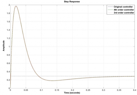
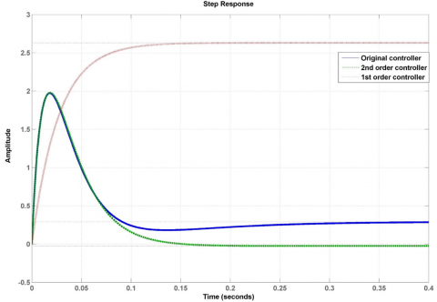
Applying the algorithm in section 2 to model (15), the results are as follows: The h(t) response and the bode response of the controllers are shown in the Figures 1 and 2.
(a) Bode response results of the 4th order controller and 3rd order controller
(b) Bode response results of the 2nd order controller and 1st order controller
Figure 1. Response results h(t) of the controllers
(a) Bode response results of the controllers 4th order controller and 3rd order controller
(b) Bode response results of the controllers 2nd order controller and 1st order controller
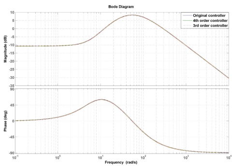
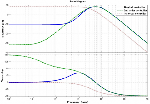
Figure 2. Bode response results of the controllers
3.2 Discussion
As mentioned in section 2, the algorithm is capable of classifying and ordering the poles of the system based on the value of the dominance index $H \infty$, specifically the decreasing order of the dominant poles is as follows: -37.428; -75.548; -12.183; -0.847; -345.692.
From the results of Table 1, it can be seen that when removing the less dominant poles (-0.847; -345.692), the order reduction error is very small. The order reduction error of the 4th order controller and the 3rd order controller is very small.
Table 1. The order reduction result of the controller (15)
|
Order |
$\boldsymbol{R}_r(\boldsymbol{s})$ |
$\operatorname{Error}\left\|R(s)-R_r(s)\right\|_{H_{\infty}}$ |
The Poles |
|
4 |
$\frac{303 s^3+3387 s^2+1.279 .10^4 s+8422}{s^4+126 s^3+4310 s^2+3.801 .10^4 s+2.919 .10^4}$ |
0.0110 |
-75.548 -37.428 -12.183 -.847 |
|
3 |
$\frac{303 s^2+3131 s+1.012 .10^4}{s^3+125.2 s^2+4204 s+3.445 .10^4}$ |
0.0115 |
-75.548 -37.428 -12.183 |
|
2 |
$\frac{299.1 s-73.15}{s^2+113 s+2828}$ |
0.7891 |
-75.548 -37.428 |
|
1 |
$\frac{98.45}{s+37.43}$ |
16.3439 |
-37.428 |
When removing the more dominant poles (-75.54; -12.183), the order reduction error increases very much. Specifically, when removing the dominant pole (-12.183) of the 3rd order system to obtain the 2nd order controller, the error of this controller increased by 68.6 times (0.789/0.0115) compared to the error of the 3rd order controller. Continuing to remove the dominant pole (-75.548) of the 2nd order controller to obtain the 1st order controller, the error of this controller increased by 20.7 times (16.343/0.789) compared to the error of the 2nd order controller.
From the results and Figure 1, we see the order of the important extreme points is arranged in decreasing order as follows: -37.4281; -75.5484; -12.1837; -0.8472; -345.6925.
The h(t) response of the original controller, the 4th order controller and the 3rd order controller are completely identical.
The h(t) response of the original controller and the 2nd order controller has a deviation in the steady-state region.
The response h(t) of the first-order controller deviates greatly from the response h(t) of the original controller.
Thus, the response error h(t) of the reduced order systems with the original system in Figure 1 is similar to the reduced order error results in Table 1.
The results of Figure 2 show that:
The bode response of the 4th order controller, the 3rd order controller and the original controller are completely identical.
The frequency amplitude response (FAR) of the original controller and the 2nd order controller are almost identical in the region w>49.8 rad/s, from the region w<49.8 rad/s, the FAR of the 2nd order controller is different from the FAR of the original controller, the lower the frequency w, the greater the difference between the two responses.
The frequency phase response (FPR) of the original controller and the 2nd order controller is almost identical in the region w>16.8 rad/s, from the region w<16.8 rad/s, the FPR of the 2nd order controller is different from the FPR of the original controller, the lower the frequency w, the greater the difference between the two responses.
The FAR of the first-order controller and the 5th order controller are completely different.
The FPR of the first-order controller and the original controller are almost identical in the region w<0.081 rad/s and w>6.103 rand/s, in the region w<0.081 rad/s<w <6.103 rand/s, the FPR of the first-order controller and the 5th order controller has a large deviation.
From the above results, it can be seen that the results in Figure 2 are similar to the reduced-order error results in Table 1.
Therefore, the original controller can be replaced by a 4th order controller or a third-order controller. The original controller can be replaced by a second-order controller if small deviations of the h(t) response and the bode response are acceptable.
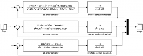
To clearly see the quality of the control system when using the controllers, a simulation model of the robust control system for the inverted pendulum is built in MATLAB-Simulink software, specifically as Figure 3.
Figure 3. Simulation diagram of inverted pendulum model control system
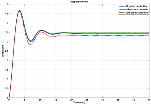
The simulation results are shown in Figure 4.
Figure 4. Control system output results
The comparison of the control system outputs is shown in Table 2.
Table 2. The control system response quality index
|
Quality Index |
Original Controller |
4th Order Controller |
3rd Order Controller |
|
Number of oscillations |
5 |
5 |
5 |
|
Overcorrection amount (maximum value) |
35.2% (4.664) |
34.4% (4.6692) |
38.7% (4.6167) |
|
Transition time |
8.35 |
8.333 |
10.96 |
|
Established value |
3.45 |
3.475 |
3.328 |
From the results in Figure 4 and Table 2, it can be seen that: Using the 4th order controller and the 5th order controller, the control system has almost similar output response and output response quality indexes.
The response of the control system using the 3rd order controller is much different from the response of the control system using the 5th order controller. The response quality indexes of the control system using the 3rd-order controller are much different from the quality indexes of the control system using the 5th order controller. Specifically, the control system using the 3rd-order controller has a large amount of overshoot, a large transition time, and a lower steady-state value than the control system using the 5th order controller.
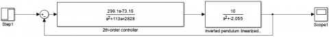
The Matlab-Simulink is used to simulate the control system using the second-order controller in Table 1 as shown in Figure 5 below:
Figure 5. Simulation diagram of the control system using a second-order controller
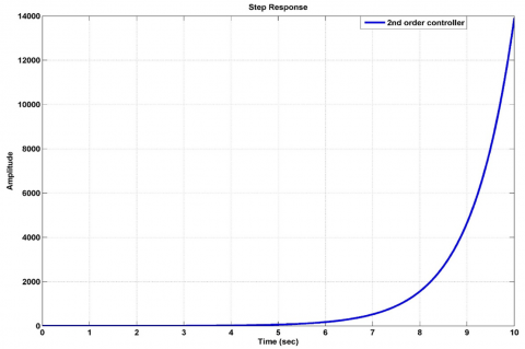
The simulation results in Figure 6 show that the control system using the 2nd order controller is not capable of stabilizing the inverted pendulum model.
Figure 6. Output results of the control system using the 2nd order controller
Thus, using a 4th order controller in the control system will ensure that the quality of the control system is maintained as when using the original controller. The 3rd, 2nd and 1st order controllers are not suitable to replace the original controller.
The above results show that the order reduction algorithm preserving the dominant pole has the ability to effectively reduce the order in the problem of reducing the order of high-order robust controllers. Combining the robust controller design method with the order reduction algorithm based on the preservation of dominant poles is an effective method for designing low-order robust controllers. The greatest advantage of the order reduction algorithm based on the preservation of dominant poles is the ability to easily and conveniently classify and arrange the poles on the main diagonal of the system matrix A.
The paper introduced the algorithm for reducing the order preserving the dominant poles based on the $H \infty$-norm. Applying the algorithm to find a suitable controller to replace the original controller in the inverted pendulum model sustainable control problem shows that the 4th-order controller is a suitable controller. The simulation results of the control system using the 4th-order controller have demonstrated the theoretical and simulation correctness of the algorithm for reducing the order preserving the dominant poles based on the $H \infty$-norm. However, our study only verifies the effectiveness of this algorithm on the simulation model. To confirm the feasibility of this algorithm, in future studies, we will conduct experiments applying the algorithm on real models or real systems.
The authors gratefully acknowledge Thai Nguyen University of Technology, Vietnam, for supporting this work. This study was not supported by any research grant or scientific project.
[1] Moore, B. (2003). Principal component analysis in linear systems: Controllability, observability, and model reduction. IEEE Transactions on Automatic Control, 26(1): 17-32. https://doi.org/10.1109/TAC.1981.1102568
[2] Antoulas, A.C. (2005). Approximation of large-scale dynamical systems. Society for Industrial and Applied Mathematics. https://doi.org/10.1137/1.9780898718713
[3] Glover, K. (1984). All optimal Hankel-norm approximations of linear multivariable systems and their L,∞-error bounds. International Journal of Control, 39(6): 1115-1193. https://doi.org/10.1080/00207178408933239
[4] Pernebo, L., Silverman, L. (2003). Model reduction via balanced state space representations. IEEE Transactions on Automatic Control, 27(2): 382-387. https://doi.org/10.1109/TAC.1982.1102945
[5] Stykel, T. (2004). Gramian-based model reduction for descriptor systems. Mathematics of Control, Signals and Systems, 16(4): 297-319. https://doi.org/10.1007/s00498-004-0141-4
[6] Stykel, T. (2006). Balanced truncation model reduction for semidiscretized Stokes equation. Linear Algebra and Its Applications, 415(2-3): 262-289. https://doi.org/10.1016/j.laa.2004.01.015
[7] Sandberg, H. (2008). Model reduction of linear systems using extended balanced truncation. In 2008 American Control Conference, Seattle, WA, USA, pp. 4654-4659. https://doi.org/10.1109/ACC.2008.4587229
[8] Vu, N.K., Nguyen, H.Q. (2021). Model reduction of unstable systems based on balanced truncation algorithm. International Journal of Electrical and Computer Engineering, 11(3): 2045-2053. http://doi.org/10.11591/ijece.v11i3.pp2045-2053
[9] Desai, U., Pal, D. (2003). A transformation approach to stochastic model reduction. IEEE Transactions on Automatic Control, 29(12): 1097-1100. http://doi.org/10.1109/TAC.1984.1103438
[10] Green, M. (2002). A relative error bound for balanced stochastic truncation. IEEE Transactions on Automatic Control, 33(10): 961-965. http://doi.org/10.1109/9.7255
[11] Opdenacker, P.C., Jonckheere, E.A. (2002). A contraction mapping preserving balanced reduction scheme and its infinity norm error bounds. IEEE Transactions on Circuits and Systems, 35(2): 184-189. http://doi.org/10.1109/31.1720
[12] Jonckheere, E., Silverman, L. (2003). A new set of invariants for linear systems--Application to reduced order compensator design. IEEE Transactions on Automatic Control, 28(10): 953-964. http://doi.org/10.1109/TAC.1983.1103159
[13] Koumir, M., El-Amrani, A., Boumhidi, I. (2021). Model reduction design for continuous systems with finite frequency specifications. International Journal of Electrical and Computer Engineering, 11(5): 3956-3963. http://doi.org/10.11591/ijece.v11i5.pp3956-3963
[14] Finecomes, S.A., Gebre, F.L., Mesene, A.M., Abebaw, S. (2022). Optimization of automobile active suspension system using minimal order. International Journal of Electrical and Computer Engineering, 12(3): 2378-2392. http://doi.org/10.11591/ijece.v12i3.pp2378-2392
[15] Hasan, M.H.C., Hassan, M.K., Ahmad, F., Marhaban, M.H., Haris, S.I., Arasteh, E. (2024). Simplifying the electronic wedge brake system model through model order reduction techniques. Bulletin of Electrical Engineering and Informatics, 13(2): 893-904. https://doi.org/10.11591/eei.v13i2.5815
[16] Swain, S., Khuntia, P.S. (2014). Design of a reduced order robust convex controller for flight control system. International Journal of Electrical and Computer Engineering, 8(2): 424-429.
[17] Thanh, B.T., Trung, N.K. (2022). Using the model reduction techniques to find the low-order controller of the aircraft's angle of attack control system. Journal Européen des Systèmes Automatisés, 55(5): 649-655. https://doi.org/10.18280/jesa.550510
[18] Dehkordi, V.R., Aghdam, A.G. (2005). A computationally efficient algorithm for order-reduction of IIR filters using control techniques. In Proceedings of 2005 IEEE Conference on Control Applications, 2005. CCA 2005, Toronto, ON, Canada, pp. 898-903. https://doi.org/10.1109/CCA.2005.1507243
[19] Hai, B.H. (2022). Applying model order reduction algorithm for control design of the digital filter. International Journal of Engineering Trends and Technology, 70(11): 288-294. https://doi.org/10.14445/22315381/IJETT-V70I11P231
[20] Aoki, M. (1968). Control of large-scale dynamic systems by aggregation. IEEE Transactions on Automatic Control, 13(3): 246-253. https://doi.org/10.1109/TAC.1968.1098900
[21] Commault, C. (1981). Optimal choice of modes for aggregation. Automatica, 17(2): 397-399. https://doi.org/10.1016/0005-1098(81)90059-5
[22] Rommes, J. (2007). Methods for eigenvalue problems with applications in model order reduction, Doctoral dissertation, Universiteit Utrecht.
[23] Rommes, J., Sleijpen, G.L. (2008). Convergence of the dominant pole algorithm and Rayleigh quotient iteration. SIAM Journal on Matrix Analysis and Applications, 30(1): 346-363. https://doi.org/10.1137/060671401
[24] Vu, N.K., Nguyen, H.Q. (2021). Model order reduction algorithm based on preserving dominant poles. International Journal of Control, Automation and Systems, 19(6): 2047-2058. https://doi.org/10.1007/s12555-019-0990-8
[25] Kang, H., Yuan, Q., Su, X., Guo, T., Cong, Y. (2024). Modal truncation method for continuum structures based on matrix norm: Modal perturbation method. Nonlinear Dynamics, 112(13): 11313-11328. https://doi.org/10.1007/s11071-024-09628-2
[26] Suman, S.K. (2024). A new scheme for the approximation of linear dynamical systems and its application to controller design. Circuits, Systems, and Signal Processing, 43(2): 766-794. https://doi.org/10.1007/s00034-023-02503-2
[27] Khansah, H. (2007). Sur la commande de systèmes non linéaires par gains robustes séquencés, Doctoral dissertation, Université Paul Sabatier-Toulouse III.
[28] Salah, A.A.H., Bouzrara, K., Garna, T., Messaoud, H. (2013). Controller order reduction techniques for loop shaping procedure. In 2013 International Conference on Electrical Engineering and Software Applications, Hammamet, Tunisia, pp. 1-5. https://doi.org/10.1109/ICEESA.2013.6578417