Salima Attache*![]() | Mohamed Sayah
| Mohamed Sayah![]() | Labib Sadek Terrissa
| Labib Sadek Terrissa![]() | Noureddine Zerhouni
| Noureddine Zerhouni![]()
© 2025 The authors. This article is published by IIETA and is licensed under the CC BY 4.0 license (http://creativecommons.org/licenses/by/4.0/).
OPEN ACCESS
Since passive earth pressure coefficients, which are impacted by wall geometry and soil properties, have an impact on wall stability, their prediction is essential to the design of retaining structures. Furthermore, the analytical and experimental methods are frequently imprecise and complicated in the context of real life. Concerning this research, three various recurrent neural network configurations, such as Recurrent Neural Network (RNN), Long Short-Term Memory (LSTM), and Gated Recurrent Unit (GRU) models were developed and evaluated for the passive earth pressure coefficients (Kpγ, Kpq, and Kpc) prediction based on Gaussian augmented data sets consisting of 671 data points. Those data sets comprised significant parameters such as the ratio of the backfill inclination angle to the internal friction angle (β/ϕ), the ratio of the friction angle of the soil-wall interface to the internal friction angle (δ/ϕ), and the angle of internal friction of the soil (ϕ). The findings demonstrate that our deep neural network models perform better than earlier methods in terms of accuracy and reliability. Thus, in terms of prediction accuracy and precision, the LSTM model performed better than the RNN and GRU models, showing the best MSE performance (Kpγ=0.00039, Kpq=0.0020, Kpc=0.0017). A sensitivity analysis shows that the wall dimensions are the most influential parameters across all models. In addition, the GRU model is the fastest in term of complexity (0.035). These results demonstrate the potential of deep learning models, particularly LSTM, to enhance geotechnical engineering design processes through improved prediction accuracy, reliability and cost-effective alternative to traditional methods.
passive earth pressure coefficient, retaining walls, data driven systems, deep learning, predictive modeling, geotechnical engineering, cost-effective analysis
The prediction of passive earth pressure is a fundamental aspect of geotechnical engineering, playing a critical role in the design and construction of retaining walls, tunnels, and other earth-supported structures. Passive earth pressure refers to the lateral force exerted by soil against a structural surface, such as a retaining wall, when the wall moves toward the soil. These pressures are influenced by several factors, including the soil-wall interface friction angle, wall geometry, backfill slope and the internal soil friction angle. Accurate estimation of passive earth pressure coefficients is crucial: underestimations can lead to structural failures, while overestimations may result in overly conservative and cost-intensive designs. Traditional methods for estimating these pressures namely analytical, experimental, and numerical approaches have significant limitations. Analytical methods, though widely used, rely on rigid and idealized assumptions that fail to capture the inherent heterogeneity and complexity of real soil behavior. Experimental techniques, while valuable, are constrained by issues of scalability, high implementation costs, and variability in soil properties, which limit the generalizability of results. Numerical methods (such as finite element and finite difference techniques) offer greater flexibility, but their reliability is highly dependent on mesh quality, the selection of appropriate constitutive models, and the availability of robust validation data. Moreover, they often entail substantial computational demands [1-17].
In response to these challenges, machine learning (ML) has gained traction in geotechnical engineering for its ability to model complex, nonlinear systems without relying on explicit assumptions. ML models, driven by data rather than predefined equations, can uncover intricate patterns and provide predictive insights across various engineering domains. Many researches have successfully applied ML techniques such as decision trees, Support Vector Machine (SVM), and ensemble methods to problems involving soil classification, slope stability, and foundation design [18-26].
More recently, deep learning has become as a transformative technology in the field, offering enhanced capabilities over traditional ML through its use of multilayered neural architectures. Deep learning (DL) models like Artificial Neural Network (ANN), CNN, and Recurrent Neural Network (RNN) have demonstrated superior performance dealing with spatial and temporal complexities inherent in geotechnical systems. Applications range from tunnel deformation prediction [27-31] and landslide susceptibility mapping [32-34] to soil property estimation [35-40], slope stability [41], and pile bearing capacity prediction [42-45].
In particular, RNN-based models such as Gated Recurrent Unit (GRU), Long Short-Term Memory (LSTM) networks are well-suited for modeling sequences and temporal data, yet remain underutilized in soil-structure interaction problems. Despite the proliferation of DL methods across geotechnical domains, there is a notable gap in their application to passive earth pressure prediction. While a few research explored the use of AI for retaining wall stability and design optimization [46-53], none have specifically addressed the use of RNN, LSTM, or GRU architectures for estimating passive earth pressure coefficients.
Gao et al. [28] used three different methods: RNNs, LSTM networks, and GRU networks to determine the best model of a GRU in the prediction of earth pressure of tunnel boring machines (TBM) operating parameters based on TBM in-situ operating data. Gao et al. [29] proposed a deep learning-based framework to predict and automatically regulate earth pressure during shield tunneling. GRU models have also been integrated with genetic algorithms to develop real-time dynamic earth pressure regulation systems for shield tunneling. In the study conducted by Hsu et al. [46], an AI-based methodology for accurately predicting displacements of retaining walls during deep excavation has been studied. When it comes to accurately predicting displacements at predefined observation points, peak wall displacements, and their corresponding positions, the multilayer functional-link network outperforms the conventional backpropagation neural network (BPNN). Nguyen et al. [47] developed a soft computing model to accurately estimate active pressure behind rigid retaining walls, including the effects of negative wall soil friction, which demonstrated strong alignment with measured values. This method offers a practical tool for retaining wall design and analysis. In reference [49], the researchers employed machine learning models including: Feed-Forward Neural Network Backpropagation (FFNN-BP), Long Short-Term Memory (LSTM), Bidirectional LSTM (Bi-LSTM), and Support Vector Regression (SVR) using real-world data from a high-rise building's excavation site, they employed a walk-forward validation technique to assess model performance. Among the models, Bi-LSTM demonstrated superior accuracy and robustness in predicting wall deflections, outperforming the others.
In this paper, we propose a novel deep learning-based framework for passive earth pressure coefficients $({{K}_{p\gamma }}$,$\text{ }\!\!~\!\!\text{ }{{K}_{pq}}$ and ${{K}_{pc}})$ prediction with improved accuracy and efficiency. We develop and evaluate three deep learning models (RNN, GRU, and LSTM) using a dataset composed of key geotechnical parameters, including the ratio of backfill inclination angle to the internal friction angle $(\beta /\phi )$, the soil-wall interface friction angle to internal friction angle ratio ($\delta /\phi )$, and the soil friction angle ($\phi )$. Beyond standard training procedures, an innovative hyperparameter tuning algorithm is employed to optimize model performance. We assess the models using multiple metrics: mean squared error (MSE), coefficient of determination (R²), and score function. We also have introduced a novel ranking approach to compare model performance across the different coefficients. Finally, computational cost, model complexity, and sensitivity analyses have been performed to evaluate the practical applicability of each model.
The structure of this article is as follows: The methodological basis of our inquiry is presented in Section II after the introduction. The formulation of the problem as well as the theoretical background of the three models have then been thoroughly explained. The experimental investigation is described in Section III, which also provides the hyper-parameter configuration, performance assessment metrics, and data description. Section IV provides a full discussion of our investigation's findings along with sensitivity analysis and computational cost and complexity. In Section V, the conclusion and perspectives are finally presented.
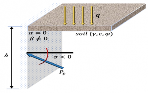
The purpose of main study predicting the passive earth pressure coefficients of a vertical rough rigid retaining wall with an inclined ground surface (Figure 1). The passive earth pressure ${{P}_{p}}$ acting on this wall can be expressed in terms of earth pressure coefficients ${{K}_{p\gamma }}$,$~{{K}_{pq}}$ and ${{K}_{pc~}}$according to Eq. (1).
${{P}_{p}}=\frac{\gamma {{h}^{2}}}{2}b{{K}_{p\gamma }}+qhb{{K}_{pq}}+chb{{K}_{pc~}}$ (1)
where, $h\text{ }\!\!~\!\!\text{ }$is the height of retaining wall ($h=1$ m$)$, $b\text{ }\!\!~\!\!\text{ }$is the breadth of the wall, $\gamma $ is the unit weight of soil, $c\text{ }\!\!~\!\!\text{ }$is the soil cohesion, and $q\text{ }\!\!~\!\!\text{ }$is the surcharge on the ground surface. The coefficients of passive earth pressure resulting from soil weight, surcharge loading, and cohesion are denoted by ${{K}_{p\gamma }}$,$\text{ }\!\!~\!\!\text{ }{{K}_{pq}}$ and ${{K}_{pc\text{ }\!\!~\!\!\text{ }}}$, respectively.
Based on collected data, this research uses machine learning techniques and suggests an efficient way to predict with accuracy the passive earth pressure coefficients. Figure 2 gives the synoptic schema of the proposed solution. An offline stage is proposed where the AI model is trained and validated, and then an online stage is introduced model for testing where the passive earth coefficients are predicted. The solution is built upon three phases: (1) Data preparation, (2) Data processing, and (3) Results. After collecting and structuring the raw data, we proceeded to visualize and analyze this data in the first phase in order to provide more insightful and representative data to the second phase for processing.
Figure 1. Rigid retaining wall
Figure 2. Synoptic schema of the proposed solution
Subsequently, in the third phase, three prediction models (RNN, LSTM, and GRU) were trained and verified to ensure that they possess the maximum degree of accuracy. The passive earth pressure coefficients can be predicted after the model has been validated and saved. In addition, the dataset is updated systematically with new values. We noticed that the online stage takes less time than the offline stage which is more time consuming to execute.
2.1 Problem formulation
Considering a predicting problem that have three parameters as an input and three coefficients as an output with ${{T}_{i}}$ values. We can define the data as:
$Dataset=({{X}^{i}},{{Y}^{i}}),\text{ }\!\!~\!\!\text{ }i=1,\text{ }\!\!~\!\!\text{ }2,\text{ }\!\!~\!\!\text{ }3,\ldots ,N$ (2)
Thus, ${{X}^{i}}$ denotes the gathered measurements matrix of the rigid retaining wall in which ${{Y}^{i}}$corresponds to the passive earth pressure coefficients as shown in Eq. (3) and Eq. (4) respectively.
${{X}^{i}}=\left[ {{x}_{1}},\text{ }\!\!~\!\!\text{ }{{x}_{2}},\text{ }\!\!~\!\!\text{ }\ldots ,\text{ }\!\!~\!\!\text{ }{{x}_{{{T}_{i}}}}\text{ }\!\!~\!\!\text{ } \right]\text{ }\!\!~\!\!\text{ }\in {{R}^{m\times {{T}_{i}}}}$ (3)
${{Y}^{i}}=\left[ {{y}_{1}},\text{ }\!\!~\!\!\text{ }{{y}_{2}},\text{ }\!\!~\!\!\text{ }\ldots ,\text{ }\!\!~\!\!\text{ }{{y}_{{{T}_{i}}}}\text{ }\!\!~\!\!\text{ } \right]\text{ }\!\!~\!\!\text{ }\in {{R}^{1\times {{T}_{i}}}}$ (4)
where, ${{T}_{i}}$ is the total instances number.
The coefficients can be calculated using the current $\left( y_{t}^{i} \right)$ as a target Eq. (5).
${{Y}_{pred}}\approx y_{t}^{i},\text{ }\!\!~\!\!\text{ }\!\!~\!\!\text{ }t=1,\text{ }\!\!~\!\!\text{ }2,\text{ }\!\!~\!\!\text{ }\ldots {{T}_{i}}$ (5)
To address the non-linearity function$\text{ }\!\!~\!\!\text{ }\left( \Phi \right)$ deep learning methods are proposed in this paper.
Let ${{X}_{i}}\text{ }\!\!~\!\!\text{ }$denote the input of the function $\left( \Phi \right)$, and the observed ${{Y}_{pred}}$ is its output. Therefore, we have:
${{Y}_{pred}}=\Phi \left( x_{t\text{ }\!\!~\!\!\text{ }}^{i},\text{ }\!\!~\!\!\text{ }y_{t}^{i} \right)$ (6)
The difference between the target coefficient that was observed and the predicted coefficient value at time$\text{ }\!\!~\!\!\text{ }t\text{ }\!\!~\!\!\text{ }$has been minimized as shown in Eq. (7)
$Minimize\text{ }\!\!~\!\!\text{ }:\left( {{Y}_{pred}},\text{ }\!\!~\!\!\text{ }y_{t}^{i} \right)$ (7)
2.2 Recurrent neural networks
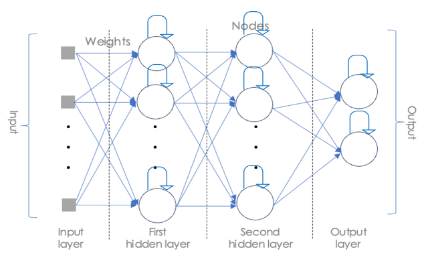
A well-known family of ANNs designed especially to process sequential data, including speech signals, text sequences, and time series data, are RNNs. RNNs include an internal memory system that allows them to remember information from prior inputs, in contrast to typical feedforward ANNs that analyze each input separately. Because of their inherent memory capacity, they perform in tasks like speech recognition, machine translation, signal analysis, and natural language processing.
The main characteristic of an RNN is its feedback loop, which enables it to transfer data across time steps. This feedback loop, typically implemented by recurrent connections between the network's hidden layers, enables the accumulation of sequential information. This internal memory allows RNNs to model temporal dependencies, understanding the relationships between inputs across time. It contains an input layer, hidden layers, and an output layer as the most fundamental kind of neural network [54].
Depending on the network's depth, there may be one or more hidden layers. Each layer has a specific number of recurrent neurons that serve as processing units; each neuron is exclusively coupled to the neurons of the layer below and its last state as shown in Figure 3.
The RNN family includes a number of different architectures, such as:
Figure 3. Recurrent neural network architecture
2.3 LSTM
RNN is a form of ANNs that can be used for all sequential and time-series data such as video frames, text, music and others. Different from the standard neuron, an RNN is a structure composed of several recurrent neurons. The main issue with RNNs is that they contain a vanishing gradient problem. Therefore, LSTMs and GRU were established to avoid backpropagated errors from vanishing or exploding by integrating their state dynamics with gating [57, 58]. The gates are implemented to avoid the long-term dependency problem and allow each recurrent unit to extract time-scale-dependencies. LSTM and GRU cells are one of the main factors contributing to RNN's recent success.
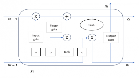
An LSTM unit is made up of four doors:
Figure 4. LSTM cell diagram
A typical LSTM cell is depicted in Figure 4. Firstly, LSTMs make modifications to the cell state in which it is divided into two states, the long-term C(t) and the short-term H(t). Second, to control the cell states, three control gates: the forget gate, the input gate, and the output gate, are inserted along the state path. The calculation equations of LSTM are as follow:
${{f}_{t}}=\delta \left( {{W}_{t}}{{x}_{t}}+{{H}_{f}}{{h}_{t-1}}+{{b}_{f}} \right)$ (8)
${{i}_{t}}=\delta \left( {{W}_{i}}{{x}_{t}}+{{H}_{i}}{{h}_{t-1}}+{{b}_{i}} \right)$ (9)
${{g}_{t}}=tanh\left( {{W}_{g}}{{x}_{t}}+{{H}_{g}}{{h}_{t-1}}+{{b}_{g}} \right)$ (10)
${{o}_{t}}=\delta \left( {{W}_{0}}{{x}_{t}}+{{H}_{0}}{{h}_{t-1}}+{{b}_{0}} \right)$ (11)
${{C}_{t}}=\left( {{f}_{t}}\text{ }\!\!~\!\!\text{ }\oplus {{C}_{t-1}} \right)\oplus ({{i}_{t}}\oplus {{g}_{t}})$ (12)
${{h}_{t}}=tanh({{C}_{t}}\oplus {{O}_{t}})$ (13)
where, ${{w}^{\text{*}}},$ ${{H}^{\text{*}}}$ and ${{b}^{\text{*}}}$ denote respectively each gate's trainable weights and biases referred to as *. Moreover,
· $\delta $: activation function,
· ${{x}_{t}}:\text{ }\!\!~\!\!\text{ }$current input,
· $i$: input gate,
· $f$: forget gate,
· $O$: output gate,
· ${{h}_{t-1}}$: previous iteration's hidden state,
· ${{C}_{t}},\text{ }\!\!~\!\!\text{ }{{C}_{t-1}}$: hidden states.
2.4 GRU
Comparable to the LSTM unit, the GRU has emerged as an improved LSTM architecture network that merges cellular state and hidden state into one state and integrates forget and input gates into a single update gate as well [59]. Mainly, two gates, known as update and reset gates, substitute the four LSTM gates in the GRU. Figure 5 shows the GRUcell architecture, whereas, the state at each time of the GRU cell is computed by the following equations:
${{z}_{t}}=\delta \left( {{W}_{zt}}{{x}_{t}}+{{H}_{z}}{{h}_{t-1}}+{{b}_{z}} \right)$ (14)
${{r}_{t}}=\delta \left( {{W}_{r}}{{x}_{t}}+{{H}_{r}}{{h}_{t-1}}+{{b}_{r}} \right)$ (15)
${{g}_{t}}=tanh({{W}_{g}}{{x}_{t}}+{{H}_{g}}\left( {{r}_{t}}\oplus {{h}_{t-1}} \right)+{{b}_{g}}$ (16)
${{C}_{t}}={{z}_{t}}\oplus {{h}_{t-1}}+\left( 1-{{z}_{t}} \right)\oplus {{g}_{t}}$ (17)
where, $\text{ }\!\!~\!\!\text{ }{{W}^{\text{*}}},$ ${{H}^{\text{*}}},\text{ }\!\!~\!\!\text{ }$and ${{b}^{\text{*}}}\text{ }\!\!~\!\!\text{ }$refer to the learnt weight matrices and biases for each gate that is designated with ${{a}^{\text{*}}},$ respectively. Moreover, the activation function is the $\delta $. The current input is ${{x}_{t}}$, and the rest and update gates are $r$ and $z$, respectively. The hidden state of the previous iteration is indicated by ${{h}_{t-1}}$, while the hidden state of the current iteration is shown by ${{h}_{t}}$.
Figure 5. GRU cell diagram
Three deep learning models RNN, GRU, and LSTM will be explored in this study. The several levels of interdependence (1) without, (2) short-term, and (3) long-term relationships have been taken into account in the material dataset. The performance of various models will be assessed and compared using the loss, val_loss, and Score S parameters. A comparative study will also be performed to determine which model is best for the passive earth pressure coefficients. The data preprocessing, hyper-parameter setup, and performance assessment metrics will be a dressed in this section.
Table 1. Statistics of the dataset
|
Parameters |
Symbol |
Min |
Max |
Mean |
Med |
|
Wall width to wall height ratio |
$\beta /\phi $ |
-0.666 |
0 |
-0.333 |
-0.333 |
|
Soil friction angle |
$\phi $ |
20 |
40 |
30 |
30 |
|
Ratio of soil wall |
$\delta /\phi $ |
0 |
1 |
0.5 |
0.5 |
|
PEP Coeff. |
${{K}_{p\gamma }}$ |
2.04 |
2.06 |
3.05 |
3.05 |
|
PEP Coeff. |
${{K}_{pq}}$ |
2.04 |
4.47 |
3.255 |
3.255 |
|
PEP Coeff. |
${{K}_{pc\text{ }\!\!~\!\!\text{ }}}$ |
2.86 |
6.77 |
4.815 |
4.815 |
3.1 Data description
Three numerical datasets with 671 instances and three parameters, were used in our investigation. These data sets are structured and arranged according to reference [3]. They include the passive earth pressure coefficients that are determined by the rigid retaining wall's characteristics and soil. The main statistical features of our datasets are displayed in Table 1. The ratio of backfill inclinisation angle to the internal friction angle $(\beta /\phi )$, the soil friction angle ($\phi $) and the Ratio of the soil wall interface friction angle to internal friction angle $\left( \delta /\phi \right)$, were considered as input parameters, while the output ones are the passive earth pressure coefficients $({{K}_{p\gamma }}$,$\text{ }\!\!~\!\!\text{ }{{K}_{pq}}$, ${{K}_{pc}})$.
In order to handle these coefficients for monovariate and bivariate analysis, we have created three independent tables.
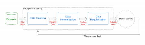
3.2 Data pre-processing
The first and most important stage in developing a machine learning mode is data preprocessing. In the field of data driven-systems, data preprocessing stage is essential to guaranteeing accurate and relevant analysis [60]. In this part, we give a thorough methodology for preprocessing our dataset, which includes a variety of variables (such as soil and wall factors in our case study).
The used techniques for data cleaning, data normalization, and regularization are all part of our data preparation procedure as shown in Figure 6.
Figure 6. Flowchart of the preprocessing pipeline
3.2.1 Data cleaning
Data cleaning is the first stage in our preparation procedure. The dataset is thoroughly examined, and any missing values, outliers, or discrepancies are noted and dealt with. By eliminating or imputing missing values and correcting incorrect entries, this stage keeps the dataset's integrity and reduces the possibility of bias in subsequent research.
3.2.2 Data standardization
It is essential to normalize the data when utilizing a dataset that can include variables measured on several scales. This may remove scale-related biases. To scale the variables to a common scale, we use data standardization techniques like min-max normalization. By ensuring that each variable contributes equally to the processing stage. This procedure makes it possible to compare variables fairly and accurately gauge how they affect the coefficients.
3.2.3 Regularization
We use regularization techniques to improve the analysis quality even further. Regularization enhances the generalizability of the models and reduces overfitting. By using regularization, we establish a penalty term that limits the complexity of the model and discourages excessive dependence on specific variables. This strategy increases the model's capacity to generalize new data and reduces the probability that it will fit noise, which improves the analysis resilience.
The process of pre-processing pipeline is depicted in Figure 6. Once the pre-processing is carried out, we will enhance the integrity, reliability, and interpretability of subsequent research by completing data cleaning, standardization, and regularization. This pre-processing pipeline provides a helpful framework for gaining insightful knowledge and understanding the connections between structure properties and passive earth pressure coefficients. Therefore, the outcomes of this phase will be more accurate and reliable for the prediction process.
3.3 Hyper-parameters setting
Although choosing the model hyper-parameters is a meticulous and expensive process, it is nevertheless crucial since it has a significant influence on the accuracy of the predictions. The hyper-parameters setting for deep models are done manually by the Error-And-Trial method in all experiments. In the following, we will set out the different hyper-parameters used in our study.
· Timesteps: refers to the sequence length in the input data,
|
Algorithm 1: Best Accuracy-Based Deep Model |
|
Data: Passive Earth Pressure Coefficients-Prediction Neural Network architecture A Dataset splitted in Xtr, Xte, ytr, yte Result: M∗ ; // Best Smart Deep Model 1 timesteps ← Input Dataset timesteps 2 features ← Input Dataset features 3 loss functions ← ’mean squared error’ 4 metrics ← ’accuracy’ 5 layer numbers ← {1, 2, 3, 4} 6 cells per layer ← {3, 6, 9, 12} 7 epochs ← {50, 100, 150, 200} 8 batch sizes ← {6, 12, 18, 24} 9 activation functions ← {’sigmoid’, ’relu’, ’softmax’, ’tanh’} 10 dropout rates ← {0.2, 0.4, 0.6, 0.8} 11 dense layers ← {1, 5, 10, 12} 12 optimizers ← {0.1, 0.01, 0.001, 0.0001} 13 params ← [timesteps, features, loss functions, metrics, layer numbers,cells per layer, epochs, batch sizes, activation functions, dropout rates, dense layers, optimizers]; For p ∈ params do 15. model=Create DeepModel(params, A) 16 // Compile model(params) 17 Eval model(params) 18 If isBest(model.loss) then 19 M∗← model; 20 End 21 End 22 return M |
• We consider the 32 samples in our raw material dataset.
• Features: Indicates the number of input distinct features measurements or attributes associated with each data point. The 12 material features were introduced as input variables for our shallow LSTM model.
• Loss functions: This function measures the dissimilarity between the predicted values and the true values during training.
• Metrics: Indicators for the evaluation of the model performance.
• Layer number: layers number in the neural network model. Instead of using a fixed number of layers, we have tested a scenario of four cases with layers number in [1, 2, 3, 4] with a fixed #cells=3. We notice that the evolution of the training and test loss functions show a perfect downhill and smoothy in the case of a LSTM model with #layers=01 and #cells=3.
• Cells by layers: The number of cells or units in the network. First of all, we have considered the parameters of a shallow LSTM model with #layers=01 and a minimum of #cells per layer.
• Epochs: Number of iterations during the training to potentially improve the model performance.
• Batch size: It describes how many samples or data points are handled during each training cycle. This batch size is used to compute the loss and update the model's weights during each training step.
• Activation function: The function that behaves as a threshold to get outputs. In our experiments, we have tested four activation functions ['sigmoid', 'relu', 'soft_max', 'tanh'] and some illustrations were done.
• Dropout rates: Used during training for regularization, to avoid overfitting. For the regularization of our shallow LSTM model.
• We have experienced four case of dropout rate in the set [0.2, 0.4, 0.6, 0.8].
• Dense layers: Standard layers where every single neuron in the preceding and next levels has connections to every other neuron.
• For the last forward dense layer, we have tested the configurations using a variation of layers in the set 1, 5, 10, 12. Here, we noticed that the adequate dense layer size is 12.
• Optimizers: Used for the configuration of the learning rate. We have used the Adam optimiser with variable learning rate.
Table 2. Hyperparameters configuration of the three models
|
Model |
Loss_Func |
Time_Steps |
Layer_Num |
Cells_by_Layer |
Epochs |
Batch_Size |
Act_Func |
Dropout_Rates |
Optimizer |
|
LSTM |
MSE |
160 |
6 |
(3,32,16,16,1) |
400 |
20 |
Relu |
0.1 |
0.0001 |
|
GRU |
MSE |
160 |
3 |
(3,64,1) |
400 |
20 |
Relu |
0.1 |
0.0001 |
|
RNN |
MSE |
160 |
5 |
(3,16,64,16,1) |
400 |
20 |
Relu |
0.1 |
0.0001 |
We have generated experimentally using (Algorithm 1) the best configuration of the three AI used models RNN, LSTM, and GRU. Table 2 depicted the optimal values of the learning parameters. We noticed that these parameters will be used along the following experimentation section. Furthermore, to overcome the lack of the real experimental data, we have applied a Gaussian augmentation to the dataset. New mutant transactions set $\left\{ t_{k}^{\text{ }\!\!'\!\!\text{ }} \right\}$ of size $k$ has been generated for at each data transaction $t$ in the neighbour space.
3.4 Evaluation of the model performance
The evaluation of the models is a crucial stage in the process of developing and validating the model. Depending on the kind of tasks (classification, regression, etc.), we could find a variety of assessment metrics. In this subsection, we will present the different metrics used in our studies [61, 62].
Mean Absolute Error (MAE): The average of the discrepancies between the actual values and the predicted ones is known as the mean absolute error. It is expressed mathematically as follows in Eq. (18):
$MAE=\frac{1}{N}\mathop{\sum }_{i=1}^{N}\left| z_{i}^{\text{ }\!\!'\!\!\text{ }}-{{z}_{i}} \right|$ (18)
Mean Squared Error (MSE): MSE is undoubtedly the most often used statistic for regression problems. It calculates the mean of the squared difference between the target value and the predicted value of the regression model (Eq. (19)).
$MSE=\frac{1}{N}\mathop{\sum }_{i=1}^{N}{{(z_{i}^{\text{ }\!\!'\!\!\text{ }}-{{z}_{i}})}^{2}}$ (19)
R-Squared (R2): is a regression metric also known as coefficient of determination. Eq. (20) provides this measure, it facilitates machine learning models comparison. The regression's ability to capture all of the variation in the target values is shown by how near ${{R}^{2}}$ is to the unit.
${{R}^{2}}=1-\frac{\mathop{\sum }_{i=1}^{N}{{(z_{i}^{\text{ }\!\!'\!\!\text{ }}-{{z}_{i}})}^{2}}}{\mathop{\sum }_{i=1}^{N}{{({{z}_{i}}-\bar{z})}^{2}}}$ (20)
Score function: The formula for the score S measurement in Eq. (21) monitors the learning's sensitivity and displays its smoothness. It is seen as a useful indication for understanding the learning process.
$S=\left\{ \begin{matrix} \propto *\left( \frac{ex{{p}^{\left| {{e}_{i}} \right|}}}{10}-1 \right)~~~~~~~~~~\left| {{e}_{i}} \right|\ge \varepsilon \\ 0~~~~~~~~~~~~~~~~~~~~~~~~~~~~~~~~~~~~~~~\left| {{e}_{i}} \right|~<\varepsilon \\ \end{matrix} \right.$ (21)
where,
$N$: sample number,
$z$: actual coefficient value,
${z}'$: predicted coefficient value (testing dataset).
Because they provide a thorough and precise analysis that makes it possible to determine which algorithm performs best in solving our issue. MSE, R2, and score function S have been chosen to evaluate our models.
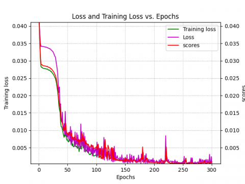
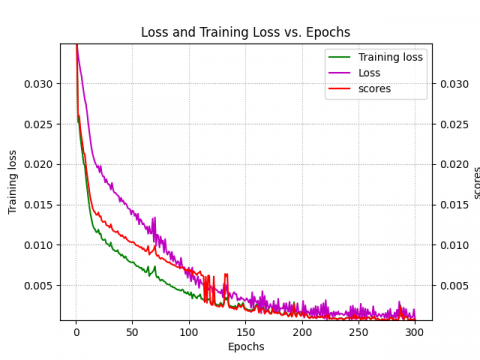
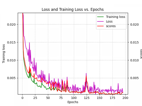
In this section, we will provide and discuss in details our prediction results. In fact, a variety of statistical tools were used to analyze and evaluate the models generated models' accuracy. We maintained the coefficient of determination ${{\text{R}}^{2}}$, the MSE, and the scoring function S. Each of these statistical metrics has been widely utilized to evaluate the precision of DL-based models [29, 61]. However, Figures 7-9 allow us to see two different stages of learning:
· A rapid learning period when the mean square error drops off fast. This stage is equivalent to identifying broad patterns in the data.
· A slower learning period, where there is a slower decline in mean square error. Learning the specifics of the data is associated with this phase.
These data also show how, as the number of learning iterations in the process grew, the loss function values for the models that were utilized quickly converged to almost zero. In the meantime, we have noticed that the RNN model's loss function stops decreasing much faster than the LSTM and GRU models. This suggests that the RNN model has reached the convergence point faster because of its simpler architecture and feedback mechanism (as shown by the score function). The models showed good convergence and were able to predict the test sets after an average of 300 iterations.
(a)
(b)
(c)
Figure 7. ${{\text{K}}_{\text{p }\!\!\gamma\!\!\text{ }}}~$loss, training loss and score vs. epochs: (a) LSTM, (b) GRU, (c) RNN
(a)
(b)
(c)
Figure 8. ${{\text{K}}_{\text{pq}}}$ loss, training loss and score vs. epochs: (a) LSTM, (b) GRU, (c) RNN
(a)
(b)
(c)
Figure 9. ${{\text{K}}_{\text{pc }\!\!~\!\!\text{ }}}$ loss, training loss and score vs. epochs: (a) LSTM, (b) GRU, (c) RNN
Eqs. (20)-(22) provide a summary of all statistical indices. The evaluation of (R2, MSE, and S) for LSTM, GRU, and RNN models concerning the three earth pressure coefficients ${{K}_{p\gamma }}$,$~{{K}_{pq}}$, and ${{K}_{pc~}}$respectively in the testing datasets are summarized in Table 3.
Table 3. Performance evaluation using different metrics
|
Models |
${{K}_{p\gamma }}$ |
${{K}_{pq~}}$ |
${{K}_{pc~}}$ |
||||||
|
MSE |
R2 |
S |
MSE |
R2 |
S |
MSE |
R2 |
S |
|
|
LSTM |
0.00037. |
0.97 |
0.00322 |
0.00019 |
0.99 |
0.00176 |
0.00017 |
0.99 |
0.00253 |
|
GRU |
0.00144 |
0.90 |
0.00237 |
0.00037 |
0.98 |
0.00107 |
0.00012 |
0.99 |
0.00188 |
|
RNN |
0.00136 |
0.90 |
0.0095 |
0.00031 |
0.98 |
0.00245 |
0.00067 |
0.96 |
0.0007 |
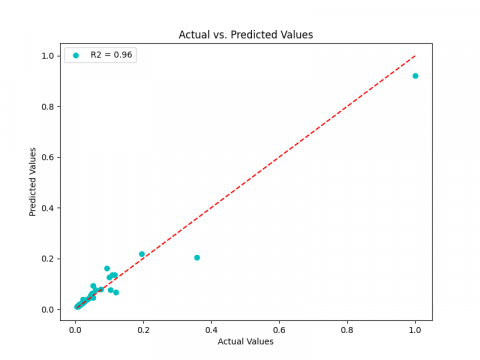
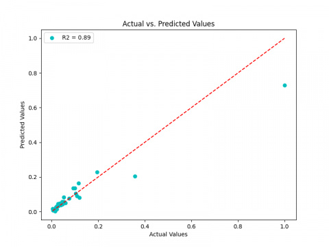
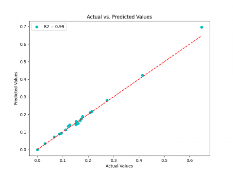
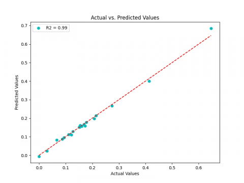
According to the MSE value, the LSTM (0.00037, 0.00019, 0.00017) provides the highest performance and outperforms RNN (0.00136, 0.00031, 0.00067), followed by the GRU (0.00144, 0.00037, 0.00012), which is still the poorest for ${{K}_{p\gamma }}$, and ${{K}_{pc}}$. RNN, however, still the worst for ${{K}_{pq}}$. Its is important to note that, in contrast to LSTM and GRU for ${{K}_{pq}}$, the LSTM and RNN models may be regarded as reliable estimators in our case study for ${{K}_{p\gamma }}$ and ${{K}_{pc}}$. Regarding the three LSTM, GRU and RNN respectively, the coefficient of determination R2 value, which are near to 1 (0.97, 0.96, 0.94) for ${{K}_{p\gamma }}$ (0.96, 0.94, 0.89) for ${{K}_{pq}}$ and (0.99, 0.99, 0.96) for ${{K}_{pc~}}$can explain this (Figures 10-12). In order to classify the performance of every model, we have additionally created the ranking technique (RT). The best accuracy (higher ${{\text{R}}^{2}}$, lower MSE and Score S) determines the best rank and consequently total score. The ranking and total scores for ${{K}_{p\gamma }},~{{K}_{pq}}$ and ${{K}_{pc~}}$for the three models are shown in Tables 4-6, respectively. It demonstrates that the LSTM model is the best predictor for all three coefficients, ranking first. In second position, we find the GRU model and RNN in the third position.
(a)
(b)
(c)
Figure 10. ${{\text{R}}^{2}}$ for ${{\text{K}}_{\text{p }\!\!\gamma\!\!\text{ }}}:\text{ }\!\!~\!\!\text{ }\!\!~\!\!\text{ }$(a) LSTM, (b) GRU, (c) RNN
(a)
(b)
(c)
Figure 11. ${{\text{R}}^{2}}$ for ${{\text{K}}_{\text{pq}}}:\text{ }\!\!~\!\!\text{ }$(a) LSTM, (b) GRU, (c) RNN
(a)
(b)
(c)
Figure 12. R2 for ${{\text{K}}_{\text{pc}}}:\text{ }\!\!~\!\!\text{ }$(a) LSTM, (b) GRU, (c) RNN
Table 4. Ranking technique for ${{K}_{p\gamma }}$
|
Models |
${{K}_{p\gamma }}$ |
$RT$ |
Total Score |
Ranking |
||||
|
MSE |
R2 |
S |
MSE |
R2 |
S |
Order |
Order |
|
|
LSTM |
37.10-5 |
0.97 |
0.032 |
3 |
3 |
1 |
7 |
1 |
|
GRU |
14.10-4 |
0.96 |
0.0023 |
1 |
2 |
2 |
5 |
3 |
|
RNN |
13.10-4 |
0.94 |
0.0009 |
2 |
1 |
3 |
6 |
2 |
Table 5. Ranking technique for ${{\text{K}}_{\text{pq}}}$
|
Models |
${{K}_{pq}}$ |
$RT$ |
Total Score |
Ranking |
||||
|
MSE |
R2 |
S |
MSE |
R2 |
S |
Order |
Order |
|
|
LSTM |
19.10-5 |
0.96 |
17.10-4 |
3 |
3 |
2 |
7 |
1 |
|
GRU |
37.10-5 |
0.94 |
0.0010 |
1 |
2 |
3 |
6 |
2 |
|
RNN |
31.10-5 |
0.89 |
0.0024 |
2 |
1 |
1 |
4 |
3 |
Table 6. Ranking technique for ${{K}_{pc}}$
|
Models |
${{K}_{pc}}$ |
$RT$ |
Total Score |
Ranking |
||||
|
MSE |
R2 |
S |
MSE |
R2 |
S |
Order |
Order |
|
|
LSTM |
17.10-5 |
0.99 |
25.10-4 |
2 |
3 |
1 |
6 |
2 |
|
GRU |
12.10-5 |
0.99 |
18.10-4 |
3 |
3 |
2 |
8 |
1 |
|
RNN |
67.10-5 |
0.96 |
7.10-4 |
1 |
1 |
3 |
5 |
3 |
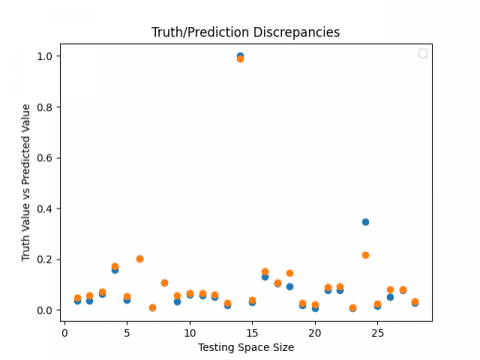
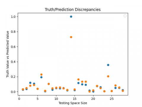
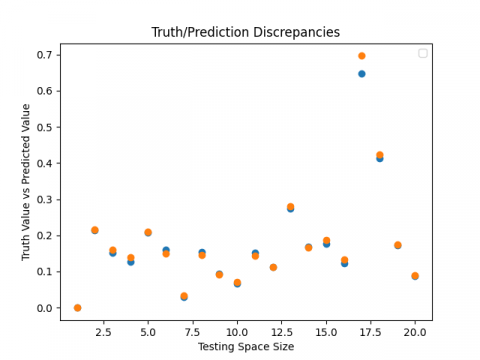
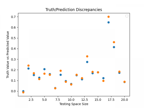
Finally, the three suggested models (LSTM, GRU, RNN) each offer a good estimator for the passive earth pressure coefficients as they have a great overall prediction (Figures 13-15) and are able to predict these coefficients precisely in an intelligent and reliable approach.
(a)
(b)
Figure 13. ${{\text{K}}_{\text{p }\!\!\gamma\!\!\text{ }}}$ truth vs. predicted values: (a) LSTM, (b) GRU, (c) RNN
(a)
(b)
(c)
Figure 14. ${{\text{K}}_{\text{pq}}}$ truth vs. predicted values: (a) LSTM, (b) GRU, (c) RNN
(a)
(b)
(c)
Figure 15. ${{\text{K}}_{\text{pc}}}$ truth vs. predicted values: (a) LSTM, (b) GRU, (c) RNN
The Tables 7-9 show the comparison between the predicted passive earth pressure coefficients ${{K}_{p\gamma }}$,$\text{ }\!\!~\!\!\text{ }{{K}_{pq}}$ and ${{K}_{pc\text{ }\!\!~\!\!\text{ }}}$ obtained from our best model (LSTM) and the corresponding results reported by reference [3] (Three-dimensional finite element limit analysis method) for various values of $\beta /\phi $, $\delta /\phi \text{ }\!\!~\!\!\text{ }$and $\phi $. In this comparison, we introduced an evaluation metric gap that takes one of two values.
The value 0, if the predicted coefficient is lower than the numerical and analytical values, or the difference between the $Min$ and the predicted coefficient, otherwise. $Min$ represents the minimum value between numerical and analytical values. Let define the variables for the experimental estimates introduced respectively in references [3, 5] as b, s thus $Min=\text{min}\left( b,s \right)$ and then gap could be defined by the Eq. (22), where, the variable $p$ represents the predicted coefficient values using the proposed AI model.
$gap=\left\{ \begin{matrix} 0~~~~~~~~~~~~~~if~~~~~~p\le \left[ Min\left( s,b \right) \right] \\ \left| p-Min\left( s,b \right) \right|~~~~~Otherwise \\ \end{matrix} \right.$ (22)
We can clearly observe that:
· For ${{K}_{p\gamma }}$, in Table 7, we notice that 82% of predicted value are consistently lower than the estimated ones in the literature [3] which reliably improves the outcomes from the analytical approaches. Again, the remaining 18% transactions ${{t}_{i,i\in \left\{ 3,\text{ }\!\!~\!\!\text{ }5,\text{ }\!\!~\!\!\text{ }6,\text{ }\!\!~\!\!\text{ }8,\text{ }\!\!~\!\!\text{ }16 \right\}}}$ of our results have slightly exceed the minimal value [3]. In this latter case, the difference or the gap does not exceed an average of 0.75 which can be considered in this case as insignificant.
· Table 8 depicts the ${{K}_{pq}}$ predicted coefficient, most of the forecasted ${{K}_{pq}}$values are under the estimated ones considering the difference $gaps$ for the transactions ${{t}_{i,i\in \left\{ 3,\text{ }\!\!~\!\!\text{ }13,\text{ }\!\!~\!\!\text{ }\!\!~\!\!\text{ }24 \right\}}}$ given in the references [3]. We notice that the predicted coefficient exceeds slightly and lays just around the zero. This means that our proposed AI model does best performance than the other approach in the literature.
· For the ${{K}_{pc\text{ }\!\!~\!\!\text{ }}}$ coefficient (see the Table 9), all the predicted values are comparatively less than the figured-out ones [3] and the prediction of this coefficient has been right over all the transactions (≈100%).
Table 7. ${{\text{K}}_{\text{p }\!\!\gamma\!\!\text{ }}}$: Predicted values vs. analytical values
|
$Id$ |
$\beta /\phi $ |
$\delta /\phi $ |
$\phi $ |
Gap Pred vs. (*) |
Predicted (Pred) |
Kinematical Approach [3] |
|
1 |
0,000 |
0,000 |
20 |
0 |
1.74 |
2.04 |
|
2 |
0,000 |
0,333 |
20 |
0 |
2.39 |
2.39 |
|
3 |
0,000 |
0,667 |
20 |
0,162 |
2.91 |
2.75 |
|
4 |
-0,500 |
1,000 |
20 |
0 |
2.14 |
2.16 |
|
5 |
-0,667 |
1,000 |
20 |
0 |
1.83 |
1.83 |
|
6 |
-0,500 |
0,000 |
25 |
0 |
1.68 |
1.71 |
|
7 |
-0,667 |
0,500 |
25 |
0 |
1.86 |
1.75 |
|
8 |
-0,333 |
0,667 |
25 |
0,108 |
2.87 |
2.77 |
|
9 |
-0,667 |
1,000 |
25 |
0 |
2.10 |
2.17 |
|
10 |
0,000 |
0,333 |
30 |
0 |
3.95 |
4.03 |
|
11 |
-0,333 |
0,333 |
30 |
0,04 |
2.810 |
2.77 |
|
12 |
-0,333 |
0,667 |
30 |
0 |
3.49 |
3.56 |
|
13 |
-0,667 |
0,667 |
30 |
0,107 |
2.237 |
2.13 |
|
14 |
-0,500 |
0,500 |
35 |
0,092 |
3.052 |
2.96 |
|
15 |
-0,333 |
0,667 |
35 |
0 |
4.64 |
4.67 |
|
16 |
0,000 |
1,000 |
35 |
1,497 |
12.797 |
11.30 |
|
17 |
-0,333 |
1,000 |
35 |
0,032 |
6.562 |
6.53 |
|
18 |
0,000 |
0,000 |
40 |
0 |
4.23 |
4.60 |
|
19 |
-0,667 |
0,000 |
40 |
0 |
1.63 |
1.67 |
|
20 |
-0,500 |
0,500 |
40 |
0,195 |
3.725 |
3.53 |
Table 8. ${{\text{K}}_{\text{pq}}}$: Predicted values vs. analytical values
|
$Id$ |
$\beta /\phi $ |
$\delta /\phi $ |
$\phi $ |
Gap Pred vs. (*) |
Predicted (Pred) |
Kinematical Approach [3] |
|
1 |
0,000 |
0,000 |
20 |
0 |
1.77 |
2.04 |
|
2 |
0,000 |
0,333 |
20 |
1,398 |
3.778 |
2.38 |
|
3 |
-0,333 |
0,333 |
20 |
0,378 |
2.338 |
1.96 |
|
4 |
-0,500 |
0,500 |
20 |
0,023 |
1.873 |
1.85 |
|
5 |
-0,500 |
1,000 |
20 |
0,027 |
2.207 |
2.18 |
|
6 |
-0,667 |
1,000 |
20 |
0 |
1.69 |
1.87 |
|
7 |
-0,500 |
0,000 |
25 |
0 |
1.69 |
1.75 |
|
8 |
-0,500 |
0,500 |
25 |
0,022 |
2.20 |
2.18 |
|
9 |
-0,667 |
0,500 |
25 |
0,019 |
1.84 |
1.83 |
|
10 |
-0,333 |
0,667 |
25 |
0,035 |
2.825 |
2.79 |
|
11 |
-0,667 |
1,000 |
25 |
0 |
2.09 |
2.26 |
|
12 |
0,000 |
0,333 |
30 |
0 |
2.88 |
3.98 |
|
13 |
-0,333 |
0,667 |
30 |
0 |
3.57 |
3.57 |
|
14 |
-0,500 |
0,333 |
35 |
0,086 |
2.78 |
2.70 |
|
15 |
-0,500 |
0,500 |
35 |
0,041 |
3.14 |
3.10 |
|
16 |
-0,333 |
0,667 |
35 |
0 |
4.69 |
4.70 |
|
17 |
0,000 |
1,000 |
35 |
0 |
9.62 |
9.82 |
|
18 |
-0,333 |
1,000 |
35 |
0 |
6.33 |
6.31 |
|
19 |
0,000 |
0,000 |
40 |
0 |
4.41 |
4.60 |
|
20 |
-0,500 |
0,500 |
40 |
0,028 |
3.77 |
3.75 |
Table 9. ${{\text{K}}_{\text{pc}}}$: Predicted values vs. analytical values
|
$Id$ |
$\beta /\phi $ |
$\delta /\phi $ |
$\phi $ |
Gap Pred vs. (*) |
Predicted (Pred) |
Kinematical Approach [3] |
|
1 |
0,000 |
0,000 |
20 |
0 |
3.10 |
2.86 |
|
2 |
0,000 |
0,333 |
20 |
0 |
3.58 |
3.76 |
|
3 |
-0,333 |
0,500 |
20 |
0 |
3.58 |
3.59 |
|
4 |
-0,500 |
0,500 |
20 |
0 |
3.32 |
3.31 |
|
5 |
0,000 |
0,667 |
20 |
0 |
4.35 |
4.59 |
|
6 |
-0,500 |
1,000 |
20 |
0,02 |
4.25 |
4.23 |
|
7 |
-0,500 |
0,000 |
25 |
0 |
2.15 |
2.26 |
|
8 |
-0,667 |
0,500 |
25 |
0 |
3.19 |
3.20 |
|
9 |
-0,333 |
0,667 |
25 |
0 |
4.48 |
4.52 |
|
10 |
-0,667 |
1,000 |
25 |
0,601 |
4.99 |
4.39 |
|
11 |
-0,500 |
0,000 |
30 |
0 |
2.15 |
2.26 |
|
12 |
0,000 |
0,333 |
30 |
0 |
4.99 |
5.14 |
|
13 |
-0,333 |
0,333 |
30 |
0,014 |
3.85 |
3.84 |
|
14 |
-0,333 |
0,667 |
30 |
0 |
5.25 |
5.26 |
|
15 |
-0,333 |
0,667 |
35 |
0 |
6.12 |
6.23 |
|
16 |
0,000 |
1,000 |
35 |
0,624 |
12.90 |
12.28 |
|
17 |
-0,333 |
1,000 |
35 |
0 |
8.26 |
8.50 |
|
18 |
0,000 |
0,000 |
40 |
0,10 |
4.39 |
4.29 |
|
19 |
-0,667 |
0,000 |
40 |
0 |
1.67 |
1.78 |
|
20 |
-0,333 |
0,333 |
40 |
0 |
4.65 |
4.66 |
4.1 Sensitivity analysis
To get the sensitivity analysis of our LSTM, GRU, and RNN models, we have considered a holistic perturbation factor alpha applied to the testing dataset and we have computed the new predicted values. Thus, when stressing the input features for each testing timesteps, we will get a new predicted value for the coefficients ${{K}_{p\gamma }}$, ${{K}_{pq}}$, and ${{K}_{pc}}$ respectively. The sensitivity is considered as the mean of all prediction variations gaps modulo the factor alpha. The sensitivity analysis reveals that for predicting Kpc, the ratio of backfill inclination angle to the internal friction angle ($\beta /\phi $) is the most influential parameter across all models, followed by the friction angle ($\phi $) and the soil-wall interface friction angle ($\delta /\phi $). The sensitivities are relatively consistent, with the LSTM (Figure 16(a)) showing slightly higher sensitivity to ($\beta /\phi $) and ($\phi $) compared to the RNN and GRU. For ${{K}_{p\gamma }}$, the ($\beta /\phi $) parameter remains the most significant, though the RNN shows a higher sensitivity to ($\beta /\phi $) than the LSTM and GRU (Figure 16(b)). Finally, for ${{K}_{pq}}$, ($\beta /\phi $) is again the dominant factor, with LSTM and GRU models exhibiting lower sensitivity to ($\beta /\phi $) compared to RNN (Figure 16(c)).
(a)
(b)
(c)
Figure 16. Sensitivity analysis: (a) LSTM, (b) GRU, (c) RNN
4.2 Computational cost and complexity
We have conducted experiments and have measure the learning time-cost (#ltime) of the deep models by regard to the complexity of each model in terms of the number of variables (#nvars). We notice that for a hidden layer, the number of the parameters is defined by:
$\#nvars=\#cells\left( input \right)*\left( \#cells\left( L-1 \right)*~\#cells\left( Lc \right)+\#cells\left( Lc \right)*\#cells\left( Lc \right)+\#cells\left( Lc \right) \right)$ (23)
In Table 10, we introduce the performance time results considering the criteria #navrs, #ltime, #ptime, and SpeedUp/RN which respectively define the number of the weight variables in the candidate neural network, the learning time, the prediction time for a given transaction or one timestep, and finally the speed up coefficient by regard to the RNN architecture considered as the baseline neural network structure deep model. We notice that LSTM like models is faster in predicting passive earth pressure coefficients with a high speed up 2.14 for GRU (e.g., 1.15 for LSTM model). Again, the LSTM learning time is speedy (i.e., LSTM learning percentage is equal to 73% of the baseline) to the RNN model considering that is less complex.
Table 10. Learning and prediction time versus variable size complexity
|
Deep Neural Architecture |
#nvar (int) |
#ltime (s) |
Learning (%) |
#ptime (s) |
Predicting Speed up |
|
LSTM |
16209 |
35.79 |
73% |
0.065 |
1.15 |
|
GRU |
17681 |
29.94 |
87% |
0.035 |
2.14 |
|
RNN |
27281 |
26.04 |
100% (baseline) |
0.075 |
1.0 (baseline) |
The LSTM-like models (GRU and LSTM) have worst times of learning and prediction by regard to the RNN baseline model. We notice that the LSTM architectures are complex than the RNN neural structures. Again, the GRU prediction is the fastest by regard to the proposed candidate’s models.
The use of deep learning techniques in civil engineering for parameters prediction has transformed the challenges of this field. Our research is part of these challenges. Furthermore, the primary goal of this study is to predict the passive earth pressure coefficients ${{K}_{p\gamma }}$,$~{{K}_{pq}}$ and ${{K}_{pc~}}$ using a new approach based on deep learning methods that greatly enhance the values of these coefficients.
To improve the data quality as well as the prediction performance of the proposed models, an efficient data preprocessing techniques were first suggested. Following that, we built a new algorithm for hyperparameters configuration in order to maintain and improve our three recurrent deep learning models (LSTM, GRU, and RNN). These models were trained and tested on a specific dataset including the cross-validation performance boosting technique. We later evaluated the model's performance using the metrics MSE, ${{\text{R}}^{2}}$, and S in addition to a newly suggested ranking method in order to obtain an accurate evaluation of our models.
Indeed, we find that the LSTM model performed significantly better than the RNN and GRU neural networks, with the best MSE performance tuple being equal to (${{K}_{p\gamma }}$=0.00037, ${{K}_{pq}}$=0.00019,$~{{K}_{pc~}}$=0.00017). Also, For the three predicted coefficients, the ${{\text{R}}^{2}}$ estimate was around one (${{\text{R}}^{2}}$_${{K}_{p\gamma }}$=0.97, ${{\text{R}}^{2}}$_${{K}_{pq}}$=0.99, and ${{\text{R}}^{2}}$_${{K}_{pc~}}$=0.99), confirming and demonstrating the best estimation and high performance of the deep predictor models. Furthermore, the RT ranking indicates that the GRU had the second-best performance, while the RNN performed the third performance.
According to the sensitivity study, the GRU model represents the best time-cost ratio and the wall dimensions have the most impactful parameters on the three models.
In conclusion, the proposed deep models for passive earth pressure coefficients prediction have shown strong performance and a high capacity to enhance the traditional approaches and get past their difficult and complex application.
The proposed deep learning approach can be adapted to address other geotechnical engineering challenges, such as ground subsidence prediction, slope stability analysis, and foundation bearing capacity evaluation. We note that already several efforts are invested to meet these challenges and we will help to cover more aspect in engineering areas, in terms of estimation and prediction. We will then boost the potential to improve the design of retaining structures, enhance the safety of geotechnical infrastructure, and contribute to the development of more sustainable construction practices.
The sensitivity analysis shows that the wall dimensions are the most influential parameters across all models and the GRU model is the fastest in term of time-cost. Finally, the proposed AI models for passive earth pressure coefficient prediction have demonstrated good performance and a high ability to boost the classical methods and overcome their complex and challenging use. Future research should focus on integrating physical constraints within neural networks to enhance interpretability and realism, expanding datasets with field-monitored or probabilistic data, and exploring the transferability of these models to other geotechnical problems such as retaining wall design, slope stability, and deep foundation behavior. Additionally, investigating hybrid models and uncertainty-aware architectures could further improve reliability and support practical decision-making.
[1] Soubra, A.H. (2000). Static and seismic passive earth pressure coefficients on rigid retaining structures. Canadian Geotechnical Journal, 37(2): 463-478. https://doi.org/10.1139/t99-117
[2] Elsaid, F. (2000). Effect of retaining walls deformation modes on numerically calculated earth pressure. In Numerical Methods in Geotechnical Engineering, pp. 12-28. https://doi.org/10.1061/40502(284)2
[3] Soubra, A.H., Macuh, B. (2002). Active and passive earth pressure coefficients by a kinematical approach. Proceedings of The Institution of Civil Engineers-Geotechnical Engineering, 155(2): 119-131. https://doi.org/10.1680/geng.2002.155.2.119
[4] Li, X.G., Liu, W.N. (2006). Study on limit earth pressure by variational limit equilibrium method. In Advances in Earth Structures: Research to Practice, pp. 356-363. https://doi.org/10.1061/40863(195)41
[5] Benmebarek, S., Khelifa, T., Benmebarek, N., Kastner, R. (2008). Numerical evaluation of 3D passive earth pressure coefficients for retaining wall subjected to translation. Computers and Geotechnics, 35(1): 47-60. https://doi.org/10.1016/j.compgeo.2007.01.008
[6] Shiau, J.S., Thomas, C.J., Smith, C.A. (2008). A FLAC model for classical earth pressure problems. Continuum and Distinct Element Numerical Modeling in Geo-Engineering.
[7] Chen, W.F., Rosenfarb, J.L. (1973). Limit analysis solutions of earth pressure problems. Soils and Foundations, 13(4): 45-60. https://doi.org/10.3208/sandf1972.13.4_45
[8] Lancellotta, R. (2002). Analytical solution of passive earth pressure. Géotechnique, 52(8): 617-619. https://doi.org/10.1680/geot.2002.52.8.617
[9] Antão, A.N., Santana, T.G., Vicente da Silva, M., da Costa Guerra, N.M. (2011). Passive earth-pressure coefficients by upper-bound numerical limit analysis. Canadian Geotechnical Journal, 48(5): 767-780. https://doi.org/10.1139/t10-103
[10] Zhu, J.F., Xu, R.Q., Li, X.R., Chen, Y.K. (2011). Calculation of earth pressure based on disturbed state concept theory. Journal of Central South University of Technology, 18(4): 1240-1247. https://doi.org/10.1007/s11771-011-0828-x
[11] Sarath Chandra Reddy, N., Dewaikar, D.M., Mohapatro, G. (2014). Computation of passive pressure coefficients: for a horizontal cohesionless backfill with surcharge using method of slices. International Journal of Geotechnical Engineering, 8(4): 463-468. https://doi.org/10.1179/1939787913Y.0000000037
[12] Soubra, A.H., Regenass, P. (2000). Three-dimensional passive earth pressures by kinematical approach. Journal of Geotechnical and Geoenvironmental Engineering, 126(11): 969-978. https://doi.org/10.1061/(ASCE)10900241(2000)126:11(969)
[13] Nguyen, T. (2022). Passive earth pressures with sloping backfill based on a statically admissible stress field. Computers and Geotechnics, 149: 104857. https://doi.org/10.1016/j.compgeo.2022.104857
[14] Attache, S., Sayah, M., Terrissa, L.S., Zerhouni, N. (2025). Predicting passive earth pressure coefficients using deep learning techniques with computational cost and sensitivity analysis. Mathematical Modelling of Engineering Problems, 12(6): 1821-1836. https://doi.org/10.18280/mmep.120601
[15] Absi, E. (2017). Active and Passive Earth Pressure Tables. Routledge. https://doi.org/10.1201/9781315136615
[16] Krabbenhoft, K. (2018). Static and seismic earth pressure coefficients for vertical walls with horizontal backfill. Soil Dynamics and Earthquake Engineering, 104: 403-407. https://doi.org/10.1016/j.soildyn.2017.11.011
[17] Tallah, N., Boulaouad, A., Bouaicha, A. (2022). Limit analyses of the active earth pressure on rigid retaining walls under strip loading on backfills. Annales de Chimie - Science des Matériaux, 46(1): 27-35. https://doi.org/10.18280/acsm.460104
[18] van Natijne, A.L., Lindenbergh, R.C., Bogaard, T.A. (2020). Machine learning: New potential for local and regional deep-seated landslide nowcasting. Sensors, 20(5): 1425. https://doi.org/10.3390/s20051425
[19] Nguyen, G., Dlugolinsky, S., Bobák, M., Tran, V., López García, Á., Heredia, I., Malík, P., Hluchý, L. (2019). Machine learning and deep learning frameworks and libraries for large-scale data mining: A survey. Artificial Intelligence Review, 52: 77-124. https://doi.org/10.1007/s10462-018-09679-z
[20] Wang, L., Wu, C., Gu, X., Liu, H., Mei, G., Zhang, W. (2020). Probabilistic stability analysis of earth dam slope under transient seepage using multivariate adaptive regression splines. Bulletin of Engineering Geology and the Environment, 79: 2763-2775. https://doi.org/10.1007/s10064-020-01730-0
[21] Njock, P.G.A., Shen, S.L., Zhou, A., Modoni, G. (2021). Artificial neural network optimized by differential evolution for predicting diameters of jet grouted columns. Journal of Rock Mechanics and Geotechnical Engineering, 13(6): 1500-1512. https://doi.org/10.1016/j.jrmge.2021.05.009
[22] Kaloop, M.R., Bardhan, A., Kardani, N., Samui, P., Hu, J.W., Ramzy, A. (2021). Novel application of adaptive swarm intelligence techniques coupled with adaptive network-based fuzzy inference system in predicting photovoltaic power. Renewable and Sustainable Energy Reviews, 148: 111315. https://doi.org/10.1016/j.rser.2021.111315
[23] Tang, L., Na, S. (2021). Comparison of machine learning methods for ground settlement prediction with different tunneling datasets. Journal of Rock Mechanics and Geotechnical Engineering, 13(6): 1274-1289. https://doi.org/10.1016/j.jrmge.2021.08.006
[24] Wu, Z., Wei, R., Chu, Z., Liu, Q. (2021). Real-time rock mass condition prediction with TBM tunneling big data using a novel rock-machine mutual feedback perception method. Journal of Rock Mechanics and Geotechnical Engineering, 13(6): 1311-1325. https://doi.org/10.1016/j.jrmge.2021.07.012
[25] Zhang, W., Li, H., Han, L., Chen, L., Wang, L. (2022). Slope stability prediction using ensemble learning techniques: A case study in Yunyang County, Chongqing, China. Journal of Rock Mechanics and Geotechnical Engineering, 14(4): 1089-1099. https://doi.org/10.1016/j.jrmge.2021.12.011
[26] Bardhan, A., GuhaRay, A., Gupta, S., Pradhan, B., Gokceoglu, C. (2022). A novel integrated approach of ELM and modified equilibrium optimizer for predicting soil compression index of subgrade layer of dedicated freight corridor. Transportation Geotechnics, 32: 100678. https://doi.org/10.1016/j.trgeo.2021.100678
[27] Ninić, J., Freitag, S., Meschke, G. (2017). A hybrid finite element and surrogate modelling approach for simulation and monitoring supported TBM steering. Tunnelling and Underground Space Technology, 63: 12-28. https://doi.org/10.1016/j.tust.2016.12.004
[28] Gao, X., Shi, M., Song, X., Zhang, C., Zhang, H. (2019). Recurrent neural networks for real-time prediction of TBM operating parameters. Automation in Construction, 98: 225-235. https://doi.org/10.1016/j.autcon.2018.11.013
[29] Gao, M.Y., Zhang, N., Shen, S.L., Zhou, A. (2020). Real-time dynamic earth-pressure regulation model for shield tunneling by integrating GRU deep learning method with GA optimization. IEEE Access, 8: 64310-64323. https://doi.org/10.1109/ACCESS.2020.2984515
[30] Zhang, W.G., Li, H.R., Wu, C.Z., Li, Y.Q., Liu, Z.Q., Liu, H.L. (2021). Soft computing approach for prediction of surface settlement induced by earth pressure balance shield tunneling. Underground Space, 6(4): 353-363. https://doi.org/10.1016/j.undsp.2019.12.003
[31] Bagińska, M., Srokosz, P.E. (2019). The optimal ANN model for predicting bearing capacity of shallow foundations trained on scarce data. KSCE Journal of Civil Engineering, 23(1): 130-137. https://doi.org/10.1007/s12205-018-2636-4
[32] Xing, Y., Yue, J., Chen, C., Qin, Y., Hu, J. (2020). A hybrid prediction model of landslide displacement with risk-averse adaptation. Computers & Geosciences, 141: 104527. https://doi.org/10.1016/j.cageo.2020.104527
[33] Zhang, W., Li, H., Tang, L., Gu, X., Wang, L., Wang, L. (2022). Displacement prediction of Jiuxianping landslide using gated recurrent unit (GRU) networks. Acta Geotechnica, 17(4): 1367-1382. https://doi.org/10.1007/s11440-022-01495-8
[34] Kurka, M. (2024). Performance of deep learning algorithms on obtaining geotechnical properties of unconsolidated material to improve input data for regional landslide susceptibility studies. In EGU General Assembly Conference Abstracts. Copernicus Meetings, p. 16620. https://doi.org/10.5194/egusphere-egu24-16620
[35] Li, L., Jin, F., Huang, D., Wang, G. (2023). Soil seismic response modeling of KiK-net downhole array sites with CNN and LSTM networks. Engineering Applications of Artificial Intelligence, 121: 105990. https://doi.org/10.1016/j.engappai.2023.105990
[36] Li, K.Q., Yin, Z.Y., Zhang, N., Liu, Y. (2023). A data-driven method to model stress-strain behaviour of frozen soil considering uncertainty. Cold Regions Science and Technology, 213: 103906. https://doi.org/10.1016/j.coldregions.2023.103906
[37] Khatti, J., Grover, K.S. (2024). A scientometrics review of soil properties prediction using soft computing approaches. Archives of Computational Methods in Engineering, 31(3): 1519-1553. https://doi.org/10.1007/s11831-023-10024-z
[38] Karimpouli, S., Tahmasebi, P. (2019). Image-based velocity estimation of rock using convolutional neural networks. Neural Networks, 111: 89-97. https://doi.org/10.1016/j.neunet.2018.12.006
[39] Han, S., Li, H., Li, M., Luo, X. (2019). Measuring rock surface strength based on spectrograms with deep convolutional networks. Computers & Geosciences, 133: 104312. https://doi.org/10.1016/j.cageo.2019.104312
[40] Khatti, J., Grover, K.S. (2024). Estimation of intact rock uniaxial compressive strength using advanced machine learning. Transportation Infrastructure Geotechnology, 11(4): 1989-2022. https://doi.org/10.1007/s40515-023-00357-4
[41] Jiang, S.H., Zhu, G.Y., Wang, Z.Z., Huang, Z.T., Huang, J. (2023). Data augmentation for CNN-Based probabilistic slope stability analysis in spatially variable soils. Computers and Geotechnics, 160: 105501. https://doi.org/10.1016/j.compgeo.2023.105501
[42] Pham, T.A., Ly, H.B., Tran, V.Q., Giap, L.V., Vu, H.L.T., Duong, H.A.T. (2020). Prediction of pile axial bearing capacity using artificial neural network and random forest. Applied Sciences, 10(5): 1871. https://doi.org/10.3390/app10051871
[43] Khanmohammadi, M., Armaghani, D.J., Sabri Sabri, M.M. (2022). Prediction and optimization of pile bearing capacity considering effects of time. Mathematics, 10(19): 3563. https://doi.org/10.3390/math10193563
[44] Liu, F., Peng, X., Su, P., Yang, F., Li, K. (2024). Enhancing pile bearing capacity estimation through random forest-based hybridization approach. Multiscale and Multidisciplinary Modeling, Experiments and Design, 7(4): 3657-3672. https://doi.org/10.1007/s41939-024-00426-2
[45] You, R., Mao, H. (2024). Assessment of ultimate bearing capacity of rock-socketed piles using hybrid approaches. Multiscale and Multidisciplinary Modeling, Experiments and Design, 7(4): 3673-3694. https://doi.org/10.1007/s41939-024-00425-3
[46] Hsu, C.F., Wu, C.Y., Li, Y.F. (2023). Development of a displacement prediction system for deep excavation using AI technology. Symmetry, 15(11): 2093. https://doi.org/10.3390/sym15112093
[47] Nguyen, T., Shiau, J., Ly, D.K. (2024). Enhanced earth pressure determination with negative wall-soil friction using soft computing. Computers and Geotechnics, 167: 106086. https://doi.org/10.1016/j.compgeo.2024.106086
[48] Seo, S., Chung, M. (2022). Evaluation of applicability of 1D-CNN and LSTM to predict horizontal displacement of retaining wall according to excavation work. International Journal of Advanced Computer Science and Applications, 13(2): 130210. https://doi.org/10.14569/ijacsa.2022.0130210
[49] Tran, D., Nguyen, H., Wang, Y., Phan, K., Phu, T., Le, D., Nguyen, T. (2023). Analysis of artificial intelligence approaches to predict the wall deflection induced by deep excavation. Open Geosciences, 15(1): 20220503. https://doi.org/10.1515/geo-2022-0503
[50] Attache, S., Remadna, I., Terrissa, L.S., Maouche, I., Zerhouni, N. (2022). IoT based prediction of active and passive earth pressure coefficients using artificial neural networks. In International Conference on Networked Systems. Cham: Springer International Publishing, pp. 252-262. https://doi.org/10.1007/978-3-031-17436-0_17
[51] Mishra, P., Samui, P., Mahmoudi, E. (2021). Probabilistic design of retaining wall using machine learning methods. Applied Sciences, 11(12): 5411. https://doi.org/10.3390/app11125411
[52] Gordan, B., Koopialipoor, M., Clementking, A., Tootoonchi, H., Tonnizam Mohamad, E. (2019). Estimating and optimizing safety factors of retaining wall through neural network and bee colony techniques. Engineering with Computers, 35: 945-954. https://doi.org/10.1007/s00366-018-0642-2
[53] Chen, H., Asteris, P.G., Jahed Armaghani, D., Gordan, B., Pham, B.T. (2019). Assessing dynamic conditions of the retaining wall: Developing two hybrid intelligent models. Applied Sciences, 9(6): 1042. https://doi.org/10.3390/app9061042
[54] Medsker, L.R., Jain, L. (2001). Recurrent neural networks. Design and Applications, 5(64-67): 2.
[55] Sayah, M., Guebli, D., Noureddine, Z., Al Masry, Z. (2021). Deep LSTM enhancement for RUL prediction using Gaussian mixture models. Automatic Control and Computer Sciences, 55: 15-25. https://doi.org/10.3103/S0146411621010089
[56] Remadna, I., Terrissa, S.L., Sayah, M., Ayad, S., Zerhouni, N. (2022). Boosting RUL prediction using a hybrid deep CNN-BLSTM architecture. Automatic Control and Computer Sciences, 56(4): 300-310. https://doi.org/10.3103/S014641162204006X
[57] Hochreiter, S., Schmidhuber, J. (1997). Long short-term memory. Neural Computation, 9(8): 1735-1780. https://doi.org/10.1162/neco.1997.9.8.1735
[58] Chung, J., Gulcehre, C., Cho, K., Bengio, Y. (2014). Empirical evaluation of gated recurrent neural networks on sequence modeling. arXiv Preprint arXiv: 1412.3555. https://doi.org/10.48550/arXiv.1412.3555
[59] Cho, K., Van Merriënboer, B., Bahdanau, D., Bengio, Y. (2014). On the properties of neural machine translation: Encoder-decoder approaches. arXiv Preprint arXiv: 1409.1259. https://doi.org/10.48550/arXiv.1409.1259
[60] Remadna, I., Terrissa, L.S., Ayad, S., Zerhouni, N. (2021). RUL estimation enhancement using hybrid deep learning methods. International Journal of Prognostics and Health Management, 12(1).
[61] Raja, M.N.A., Jaffar, S.T.A., Bardhan, A., Shukla, S.K. (2023). Predicting and validating the load-settlement behavior of large-scale geosynthetic-reinforced soil abutments using hybrid intelligent modeling. Journal of Rock Mechanics and Geotechnical Engineering, 15(3): 773-788. https://doi.org/10.1016/j.jrmge.2022.04.012
[62] Naser, M.Z., Alavi, A.H. (2023). Error metrics and performance fitness indicators for artificial intelligence and machine learning in engineering and sciences. Architecture, Structures and Construction, 3(4): 499-517. https://doi.org/10.1007/s44150-021-00015-8