Ketaki Deshwandikar![]() | Neha Bhosale
| Neha Bhosale![]() | Radhika Bhagwat*
| Radhika Bhagwat*![]() | Prajakta Chavan
| Prajakta Chavan![]()
© 2025 The authors. This article is published by IIETA and is licensed under the CC BY 4.0 license (http://creativecommons.org/licenses/by/4.0/).
OPEN ACCESS
Stress is a very common form of mental disturbance that can arise due to various challenges encountered in daily life. Stress has become a widespread concern in today's society. Therefore, it becomes increasingly important to identify and manage stress for the mental as well as physical well-being of an individual. This paper focuses on leveraging deep learning techniques for stress identification by analyzing Electroencephalogram (EEG) data. The approach presented in this paper makes use of a hybrid deep learning model, which is a combination of Convolutional Neural Networks (CNNs), Bidirectional Long Short-Term Memory (BiLSTM), and Gated Recurrent Units (GRU). Simultaneous Task EEG Workload (STEW) dataset was used which includes 14-channel EEG recordings from 48 participants collected at 128 Hz before and after a 2.5-minute SIMKAP test, along with corresponding self-reported stress ratings on a 0-9 scale. Use of the Adam optimizer provided the highest accuracy of 85.31%. The key contribution of this paper involves the identification of a reduced set of 8 channels - comprising 6 fixed and 2 variable channels selected from the standard 14 channelled EEG setup. This reduction helps in reducing hardware complexity and enhancing user comfort.
Electroencephalogram, stress detection, STEW dataset, CNN, BiLSTM, GRU, Discrete Wavelet Transform, optimizers
A student might start experiencing stress as early as in school, due to various factors such as scoring good grades, peer pressure, and parental expectations along with balancing extracurricular activities. Over the years, an increase in stress due to academics has been observed, especially among adolescent high-school students, with 57.9% of teenagers reporting high stress and 40% experiencing very high stress [1].
The transition from high school to college may change the set of responsibilities, but it also introduces new academic pressures and many students may feel overwhelmed by the fact that they have to search for internships and build an exceptional resume. In a study carried out on 336 university students in India, around, 48.80% of participants felt that they experience academic stress at an average to a high level [2].
When a student further enters the corporate world, the stress that they experience only seems to increase and worsen their mental health. High occupational stress symptoms were reported among the teaching professionals (73.3%) and marketing professionals (83.3%) suffering from moderate to critical levels of stress [3]. In today’s hectic and competitive life, individuals fail to recognize that they are experiencing the effects of stress not just on their mental but physical state too.
If stress is left unmanaged it might lead to health issues like cardiovascular problems, diabetes, and cancer along with psychosocial issues such as depression and anxiety [4].
Due to these critical changes in the brain over a long period, the chances of abnormal cell growth increases [4]. Hence, it becomes really important for us to manage stress to avoid its long-term effects on our mental, emotional, and physical health.
The coping mechanism of every individual with stress varies, and researchers need to develop an assessment tool that will be able to record and evaluate the stress levels in every individual. Traditionally, measurement of stress has relied more on subjective methods, particularly by using self-report tools but these methods provide relatively little information compared to physiological stress indicators [5]. The four most common ways for capturing physiological signals in response to produced stimuli for recording and collecting human stress levels are Electromyography (EMG), Electrooculography (EOG), Electroencephalography (EEG), and Electrocardiography (ECG) [5].
(EEG) is a non-surgical, easy-to-work-on, and relatively inexpensive method that can be used for measuring the electrical impulses of the brain through the Central Nervous System (CNS) by the placement of a helmet or a cap with multiple electrodes on the scalp [6]. The EEG signal has been extensively employed to detect and analyse human stress [7], especially in relation to the frontal lobe [8].
As EEG offers real-time, dynamic views of brain activity, it helps in studying mental states, like wakefulness, sleep, relaxation, or stress and therefore, it is preferred by researchers [9, 10].
EEG signals undergo preprocessing to eliminate undesirable noise and artifacts like eye movements, blinks, muscle movement, sweat, etc. [9, 11, 12]. Moreover, feature extraction is performed to highlight the key attributes of EEG signals [12]. These features are then used to classify the stress level, as low, medium, or high. The model architecture is a hybrid design combining Conv1D for spatial feature extraction, BiLSTM for capturing bidirectional temporal dependencies, and GRU layers for efficient sequential learning. It includes dropout layers to mitigate overfitting and a fully connected output layer utilizing SoftMax activation for stress classification into three levels.
EEG data is high-dimensional, as there are multiple channels from which the data is extracted. The models developed by researchers might suffer from overfitting. The approach presented in this research paper performs feature extraction and aims to use data from only 8 channels (6 fixed channels and 2 variable channels) instead of all 14 channels, hence reducing the complexity for classification. The model was trained using 8 specific channels, which previously emerged as superior in distinguishing mental stress as they are located on the frontal and central lobes. Lastly, a comparative study was conducted to identify the optimizer that yields the best results.
The major contributions of this study are: 1) Reduce the number of channels used for processing. 2) Build a hybrid model for accurate classification of stress.
The structure of this paper is described below:
Section 2 provides an overview of the dataset used.
Section 3 reviews and discusses research and findings that has been conducted on EEG-based stress detection.
Section 4 describes the methodology in detail along with the channel selection and comparison of different optimizers.
In Section 5, the implications of the research have been discussed.
To conclude, Section 6 presents the final remarks of the paper.
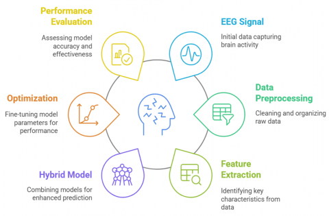
Figure 1 illustrates the processing involved in analysing EEG signals.
Figure 1. Processing
A substantial amount of research has been undertaken using machine learning algorithms like Support Vector Machine (SVM), K-Nearest Neighbour (KNN), Decision Tree, K-Means Clustering etc. [13, 14], which have shown good results. Deep learning is capable of handling complex datasets and achieving higher accuracy, which is why this study focuses on these algorithms for better results. The DEAP dataset has been thoroughly explored in previous studies but contains a relatively small number of subjects, making it unsuitable for deep learning algorithms. Therefore, the focus was shifted to the STEW dataset, which has more data points, making it a better fit for deep learning models.
Wen and Aris [15] emphasized on classifying human stress levels using EEG signals by analyzing the Theta/Beta ratio, which is associated with stress responses.
Their innovative method involved collecting brain signals from 50 university students under three experimental conditions — a resting state as the base, exposure to a 360-degree horror VR video and in the end completion of an IQ test as a cognitive stressor. After every session, the participants were given a brief time to rest and during which the induced stress was recorded. The authors then performed pre-processing to eliminate noise and artifacts, using a band-pass filter and applying Welch’s Fast Fourier Transform (FFT) algorithm to extract the Power Spectral Density (PSD) of the Theta and Beta frequency bands. The processed data was further analyzed utilizing machine learning techniques which were K-Means clustering to group participants into three classes: low, moderate and high stress. The clustering outcomes were subsequently input into a SVM classifier for stress classification. They were successfully able to prove that the Theta/Beta ratio effectively distinguishes between relaxed and stressed states, with SVM achieving an overall classification accuracy of 90%.
AlShorman et al. [16] analyzed a method for stress recognition using EEG signals from the frontal lobe. In their study, they induced stress in 14 healthy male university students through the Cold Pressor Stress (CPS) test, where participants immersed their hands in ice water. EEG data was collected using a 128-channel system and pre-processed to remove noise and artifacts using notch filters and Independent Component Analysis (ICA). They evaluated the Power spectral density using Fast Fourier Transform and for the classification of stress levels, they used two machine learning classifiers, SVM and Naive Bayes in two modes: subject-wise and mixed. Subject-wise classification achieved an impressive accuracy of 98.21%, while mixed classification reached 90% accuracy.
Tahira and Vyas [17] have come up with a hybrid deep learning model which integrates CNN and BLSTM detecting stress using EEG signals. Their research used the Physio net EEG dataset in which 19 channels were pre-processed using Discrete Wavelet Transform (DWT). CNN was employed for feature extraction and further classification of stress conditions was done using BiLSTM. Features were automatically extracted using CNN, while BLSTM was employed for classifying stress levels. Their hybrid model obtained a remarkable accuracy of 99.20%. The model built, was further validated using stratified tenfold cross-validation, yielding a classification accuracy of 98.10%.
Jawharali and Arunkumar [9] have presented an approach in which they have mainly focused on removal of Electrooculography (EOG) artifacts to enhance the accuracy for predicting human stress levels using an Artificial Neural Network (ANN) model. In their research, they have implemented a two-step process for EOG artifact removal. First, they perform EOG noise detection using an autoregressive model and then EOG noise correction through inverse filtering. This preprocessing method filters out the EOG noise from the EEG signals to a great extent. The authors have then extracted time-domain features—Simple Square Integral (SSI), Integrated EMG (IEMG), Waveform Length (WL), and Difference of Absolute Standard Deviation Value (DASDV)—to effectively classify stress. Their study used ANN to categorize stress levels into low, medium, and high, obtaining an accuracy of 91.12%.
The research conducted by Gonzalez-Vazquez et al. [18] measured mental stress levels in participants using EEG signals and a video game. The game was about controlling a car to avoid obstacles and the difficulty level kept increasing as the game progressed. They collected data from 19 participants using an 8-channel device which was processed utilizing a Recurrent Neural Network with GRUs to categorize stress into four levels–Low (0), Moderate (1), Intermediate (2), High (3). They cleaned the EEG data using techniques like filtering, normalization, and data segmentation and then for training the Adam optimizer and a categorical cross-entropy loss function were employed, achieving up to 94% accuracy for individual participants.
Tarun et al. [19] have used facial images to detect stress by analyzing expressions associated with stress, such as fear, sadness, and anger. The dataset, comprising 71,000 facial images representing seven emotions (happy, sad, angry, neutral, fear, disgust, and surprise), was pre-processed using resizing, normalization, and data augmentation to ensure consistency. The authors developed a CNN model for automatic feature extraction from these images and classify them into respective emotion categories. The CNN model was trained using the Adam optimizer and classification outputs were derived using fully connected layers with activation functions like SoftMax. Their model has achieved an accuracy of 85%, which is better as compared to previously explored methods like KNN (77.27%). The performance metrics achieved are as follows—precision is 81.82%, recall is 90.00%, and F1-score is 85.71%.
From the above study, it is evident that EEG-based stress detection has been minimally explored using deep learning approaches. The few studies that do implement deep learning rely on small-scale or self-curated datasets, lacking public availability (Table 1). This paper addresses that gap by using a larger publicly available STEW dataset. Most of the study done for classification of stress level used a single model on smaller datasets while, the proposed hybrid approach takes an advantage of the properties of each deep learning model i.e.; CNN, BiLSTM and GRU which results in improved accuracy of the hybrid model for larger dataset.
Table 1. Literature review table
|
References |
Algorithm Used |
Results |
|
[15] |
K-Means Clustering, SVM |
Accuracy = 90% using Theta/Beta for stress detection |
|
[16] |
SVM, Naive Bayes (NB) |
Subject-wise classification accuracy = 98.21%; Mixed classification accuracy = 90% |
|
[17] |
CNN, BiLSTM |
Accuracy = 99.20% |
|
[9] |
ANN |
Accuracy = 91.12% |
|
[18] |
RNN with GRUs |
Accuracy = 94% for stress classification from 8 channels |
|
[19] |
CNN |
Accuracy = 85% for stress detection using facial images |
3.1 Dataset
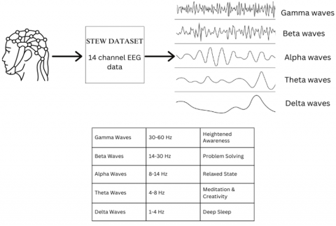
This study focuses on identifying user stress levels using the STEW dataset. The STEW dataset consists of 48 participants, where each participant took a SIMKAP test spanning 2.5 minutes each to induce stress. EEG signals were taken using the Emotiv EPOC device. The sampling frequency was 128 Hz. The dataset consists of 14 channels, each corresponding to AF3, F7, F3, FC5, T7, P7, O1, O2, P8, T8, FC6, F4, F8, and AF4, respectively. The STEW dataset consists of 2 sets of files, one before the candidates underwent the SIMKAP test indicated using subno_lo.txt file and the other after the candidates were subjected to the SIMKAP test indicated using subno_hi.txt file. (e.g., sub02_lo.txt for subject 2 at rest and sub22_hi.txt for subject 22 after the multitasking test). The rows represent the EEG signals and columns represent the 14 EEG channels. A ratings.txt file is provided that states each user’s respective stress levels on a scale of 0 to 9 before and after the conduct of the test [20].
In the STEW dataset, fifty male graduate students participated, all of whom reported no history of neurological or psychiatric disorders and had taken part in any prior EEG experiments. Data was found to be incomplete for two subjects; hence, data from only 48 subjects out of 50 has been curated in the STEW dataset. By selecting a uniform participant group, the dataset controls for demographic factors such as age, gender, education level that could otherwise introduce variability [21].
3.2 Methodology
This section outlines the methodology employed for EEG based stress detection, detailing the data preprocessing, feature extraction and model architecture used to classify stress levels accurately.
Step 1: Data preprocessing:
Data preprocessing of STEW dataset is essential to filter noise, remove artifacts, and retrieve relevant features for stress classification.
The raw EEG data is imported, and a bandpass filter is utilized which permits signals within the designated frequency and attenuates signals outside 3 Hz to 40 Hz. The method makes use of Butterworth Filter to get rid of phase distortion.
Step 2: Feature extraction and signal decomposition:
This methodology incorporates the Discrete Wavelet Transform for feature extraction. DWT is used in signal processing to decompose a signal into its frequency constituents and allows the analysis of features at different scales.
To decompose the EEG signals into wavelet coefficients (detailed and approximation coefficient) and allow the analysis of features at different scales, DWT using db4 wavelet is employed.
DWT decomposes the signal into distinct frequency components one approximation and several detail coefficients which correspond to low and high-frequency components respectively. At all decomposition levels, every channel produces independent features for the approximation and detail coefficients.
The foremost benefit of using the multiple decomposition levels of DWT is that the signal being examined can be assessed within various frequency bands. As each level provides a unique resolution of a signal, there is a growing need for understanding different aspects of brain activity.
a. Approximation Coefficients (Low frequency components): At higher levels, approximation coefficients approximate some general coarse behaviour of an EEG signal. They characterize slow, large-scale brain waves which are often linked with the deeper mental states of an individual, such as being relaxed or tense.
b. Detail Coefficients (High frequency components): Detail coefficients represent high-frequency oscillations or rapid fluctuations, which actually reflect changes in brain activity that are more immediate, fine-grained. These represent faster cognitive processes, for example attention or alertness, and are relevant in stress detection as well.
Figure 2 demonstrates how EEG signals are decomposed into different frequency bands using DWT. Each band represents the different brain activity and mental states. This decomposition helps extract features from EEG signals for stress detection.
Figure 2. Decomposed EEG signal
Along with features extracted using DWT, the statistical features are also computed. Statistical Features (from Filtered Signal): Mean, Variance, Kurtosis, Skewness.
The aforementioned statistical features provide further insight into the shape and distribution of EEG signals that might not be obtained by the DWT coefficients. These features significantly contribute to the comprehensive representation of the signal, which is pivotal for detecting patterns associated with different stress levels.
The third crucial feature that is computed is Beta Power. Using the periodogram, the power spectral density (PSD) of the signal is calculated. Beta power is computed as the sum of the PSD values in the 13-30 Hz range (frequencies associated with stress and alertness). For each channel, the Beta Power is a key feature for classification.
Step 3: Model architecture and its functionality
The architecture being developed is a hybrid model that combines CNN, BiLSTM, and two layers of GRU description of which is given below:
a) 1D Convolutional Layer: This layer facilitates the extraction of local features of EEG signals (Time series data). 128 filters of kernel size 1 are employed which helps to learn the temporal features and introduce non-linearity through ReLU activation function. MaxPooling1D layer downsamples the convolution output, reducing its spatial dimensions. In this scenario, pool size of 1 is used which does not actually down sample the data but prepares it for subsequent layers. A dropout layer of 0.2 is implemented to avoid overfitting by randomly omitting 20% of neurons during the model training process.
b) BiLSTM Layer: The number of LSTM units used in this model is 64 which are used to capture long-term dependencies in the time series data. Additionally, this layer processes the input sequence bidirectionally, both forward and backward.
c) Bidirectional GRU Layer 1: This layer is just like an LSTM but using the GRU which is more computationally efficient as well as applicable to sequential data like EEG. The number of GRU units used in this model is 64, in addition to this return_sequences=True makes the output sequence to return into the next subsequent layer.
d) Bidirectional GRU Layer 2: This is another GRU layer with the number of units 32 instead of 64.
In this layer, the value of return_sequences=False, indicating that only the final output of the sequence is passed to the next layer, rather than the full sequence. In the final recurrent layer, it is conventional to only need the final representation of the sequence for classification of stress. Dropout of 0.5 is implemented in order to mitigate overfitting by randomly deactivating 50% of the available GRU units.
e) Dense Output Layer: This is the final layer with 3 units, one for each stress levels low, medium and high, and Softmax activation is employed which converts the model’s output into probabilities for each class. This layer outputs the predicted probability distribution across the three stress levels.
By leveraging DWT for feature extraction, statistical measures for enhanced signal representation and a hybrid deep learning model, this approach ensures effective classification of stress levels. The integration of CNN, BiLSTM and GRU optimizes feature learning, enhancing the model's robustness and performance.
3.3 Functionality
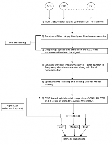
This section describes the functionality of the hybrid deep learning model, detailing how EEG features are processed, classified and mapped to stress levels based on beta power distribution. Figure 3 depicts the consolidated workflow of the model and its functionality.
Figure 3. Methodological framework
a) The input given to the deep learning hybrid model is the features that are extracted using DWT, Statistical features and the Beta Power. These features form a feature matrix for each EEG signal file. Prominent feature that is used for stress classification in 3 levels low, medium, high is Beta Power.
b) The CNN is used for spatial patterns extraction across the EEG channels. The convolutional filters traverse through the feature matrix to detect the localized patterns in beta power, including associations amongst channels or the presence of separate regional activity. These might represent changes in the distribution of beta power specific to stress conditions across various brain regions. It would be a set of feature maps that emphasize these spatial relationships as the output of this layer. Pooling is also used which helps in size reduction of feature maps, holding the most important features, which makes further computations faster.
c) BiLSTM captures temporal dependencies in the beta power sequence. The beta power values sequence is processed in both forward and backward directions to incorporate past and future context. Stress patterns are typically influenced by consistent trends and variations in beta power, here BiLSTM identifies those bidirectional temporal patterns, which helps in improving the model’s understanding of time-dependent stress indicators. The output is the overall representation of both directions, offering the detailed and richer temporal context.
d) GRU layers process and summarize the temporal features found by BiLSTM. The first GRU layer will process the output of the BiLSTM to detect simple temporal dynamics. The second GRU layer will extend the output of the first layer to detect higher-order temporal patterns. GRUs make use of gating mechanisms (update and reset gates) to selectively retain or forget information, focusing on the most stress-relevant patterns.
e) Fully Connected Dense Layers take the refined temporal and spatial features and transform them to output stress level predictions. The last GRU layer generates a feature vector which summarizes what was learned about spatial and temporal patterns. Dense layers map that vector to the three stress categories (low, medium, high). The last dense layer makes use of the Softmax activation function for producing probabilities for each class.
f) Label Assignment and Categorization of file: For each EEG file, the average beta power across all channels is calculated and stress levels are categorized using percentile-based thresholds that dynamically adapt to dataset’s distribution:
Low Stress: Beta power<33 percentile.
Medium Stress: 33rd percentile ≤ Beta power < 66th percentile.
High Stress: Average beta power > 66 percentile.
g) Training Process: The model updates its weight to reduce categorical cross-entropy loss, which quantifies the difference between predicted probabilities and the actual labels.
Optimization techniques like Adam, SGD, RMSProp, Momentum, AdaGrad, AdaDelta optimizer update the model's parameters to enhance classification accuracy.
To enhance model performance and avoid overfitting the model is trained with early stopping and learning rate reduction.
By leveraging CNN for spatial feature extraction, BiLSTM for bidirectional temporal analysis and GRU for refined sequential learning, the model effectively categorizes stress levels. Adaptive percentile-based labelling and optimization techniques ensure robust training and accurate stress classification.
This section includes performance metrics, results, and comparison of various optimizers evaluated on the hybrid deep learning models (CNN, BiLSTM, GRU). It also discusses the experimental results obtained by performing the channel selection method.
4.1 Model performance metrics
Table 2 and Table 3 showcase the model metrics obtained for the above hybrid model implemented on the STEW dataset. The accuracy obtained for the above implemented model is 85.31%.
Table 2. Confusion matrix
|
Class |
Low Stress |
Medium Stress |
High Stress |
|
C1 |
96070 |
125 |
19011 |
|
C2 |
548 |
71054 |
5202 |
|
C3 |
19251 |
1177 |
75577 |
Table 3. Model metrics and results for STEW dataset using 14 channels
|
Class |
Precision |
Recall |
F1-Score |
Support |
|
C1 |
0.83 |
0.83 |
0.83 |
115206 |
|
C2 |
0.98 |
0.93 |
0.95 |
76804 |
|
C3 |
0.76 |
0.79 |
0.77 |
96005 |
|
Macro Average |
0.86 |
0.85 |
0.85 |
288015 |
|
Weighted Average |
0.85 |
0.84 |
0.84 |
288015 |
where, C1, C2, C3 depict Low, Medium, and High stress class respectively. Support represents the number of actual instances for each class in the dataset, indicating how many samples belong to each class.
Below are the set of formulae used for calculation:
Accuracy: (CP+CN)/Total samples
Precision: CP/ (CP+IP)
Recall: CP/ (CP+IN)
F1-Score: (2 ×PR)/ (P+R)
where, CP: Correct/True Positive; CN: Correct/True Negative; IP: Incorrect/False Positive; IN: Incorrect/False Negative; Macro-Average calculates the overall precision and recall by averaging them across all classes.
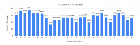
4.2 Channel selection
An experiment was performed to simplify the electrode usage during EEG signal acquisition. The model was trained using data from 8 channels only. The following six channels ['AF3', 'FC5', 'F8', 'AF4', 'P7', 'F7'] were fixed [22]. To determine the two most effective additional channels, the remaining 8 channels from the original 14-channel dataset were paired with the six channels. Figure 4 depicts the channel vs. accuracy graph derived from various channel combinations. Channel Mapping: 1: AF3, 2: F7, 3: F3, 4: FC5, 5: T7, 6: P7, 7: O1, 8: O2, 9: P8, 10: T8, 11: FC6, 12: F4, 13: F8, 14: AF4. The channels are mapped to numerical indices (e.g. AF3:1) and are referenced by these indices for ease of use in Table 4.
Figure 4. Channel combination vs. accuracy graph
Table 4. EEG channel combinations
|
A [1, 4, 13, 14, 6, 2, 3, 5] B [1, 4, 13, 14, 6, 2, 3, 7] C [1, 4, 13, 14, 6, 2, 3, 8] D [1, 4, 13, 14, 6, 2, 3, 9] E [1, 4, 13, 14, 6, 2, 3, 10] F [1, 4, 13, 14, 6, 2, 3, 11] G [1, 4, 13, 14, 6, 2, 3, 12] H [1, 4, 13, 14, 6, 2, 5, 7] I [1, 4, 13, 14, 6, 2, 5, 8] J [1, 4, 13, 14, 6, 2, 5, 9] K [1, 4, 13, 14, 6, 2, 5, 10] L [1, 4, 13, 14, 6, 2, 5, 11] M [1, 4, 13, 14, 6, 2, 5, 12] |
N [1, 4, 13, 14, 6, 2, 7, 8] O [1, 4, 13, 14, 6, 2, 7, 9] P [1, 4, 13, 14, 6, 2, 7, 10] Q [1, 4, 13, 14, 6, 2, 7, 11] R [1, 4, 13, 14, 6, 2, 7, 12] S [1, 4, 13, 14, 6, 2, 8, 9] T [1, 4, 13, 14, 6, 2, 8, 10] U [1, 4, 13, 14, 6, 2, 8, 11] V [1, 4, 13, 14, 6, 2, 8, 12] W [1, 4, 13, 14, 6, 2, 9, 10] X [1, 4, 13, 14, 6, 2, 9, 11] Y [1, 4, 13, 14, 6, 2, 9, 12] Z [1, 4, 13, 14, 6, 2, 10, 11] A1 [1, 4, 13, 14, 6, 2, 10, 12] |
Among all the channel subsets, subset D ['AF3', 'FC5', 'F8', 'AF4', 'P7', 'F7', 'F3', 'P8'] demonstrated the highest accuracy of 74.94% making it an optimal combination of 8 channels for channel reduction.
The channel reduction experimentation revealed that the reduced subset of 8 channels predominantly lie in the frontal lobe region. This further supports the relevance of channel selection, as the frontal lobe region plays a key role in the stress detection. The frontal lobe region is commonly captured across various EEG datasets making the selected channels broadly applicable across various experiments.
4.3 Optimizers comparison
A comparative analysis of the various optimizers used during the model-building process is listed below. Table 5 represents the various optimizers used, the arguments used for each respective optimizer and the accuracy obtained.
Table 5. Optimizers comparison
|
Optimizer |
Arguments Used |
Accuracy |
|
Adam |
Rate of Learning=0.001, β₁ = 0.9, β₂ = 0.999, epsilon = 1e-07, Ema momentum = 0.99 |
85.31% |
|
SGD |
Rate of Learning = 0.0005, momentum = 0.9, nesterov = True |
79.91% |
|
RMSProp |
Rate of Learning=0.0005 |
79.80% |
|
Nadam |
Rate of Learning = 0.001, β₁ = 0.9, β₂ = 0.999, Weight Decay = 1e-5, Epsilon = 1e-7 |
79.77% |
|
Adagrad |
Rate of Learning = 0.0005 |
79.43% |
|
Adadelta |
Default value |
71.90% |
|
Adadelta |
Rate of Learning = 0.0005 |
71.85% |
A comparative study demonstrates that the Adam optimizer achieved the highest accuracy of 85.31% for the model built on the 14-channeled STEW dataset. In contrast, SGD, RMSProp, Nadam and Adagrad showed a significant decline in accuracy. Adadelta has showcased a further greater loss in accuracy in comparison to Adam optimizer.
4.4 State of the art
As shown in Table 6, the proposed CNN-BiLSTM-GRU hybrid model outperforms approaches like standalone LSTM, 2D-CNN-LSTM, achieving an accuracy of 85.31%. This performance boost is likely due to the effective combination of spatial (CNN) and temporal (BiLSTM, GRU) feature extraction.
Table 6. State of the art works for stress detection
|
Model |
Dataset |
Accuracy |
|
LSTM |
DEAP |
72 % |
|
2D-CNN-LSTM |
STEW |
72.55% |
|
CNN-BiLSTM-GRU Hybrid model |
STEW |
85.31% |
In this study, a hybrid model using CNN, GRU and BiLSTM was utilized to categorize the stress levels into low, medium and high using EEG signals. The hybrid model was built on the 14-channeled STEW dataset. The hybrid model achieved an accuracy of 85.31% with the Adam optimizer performing the best in comparison to other optimizers like SGD and RMSProp. Furthermore, channel reduction was applied to identify a subset of 8 channels to reduce the signal acquisition complexity.
The stress detection model classified incorrect stress levels for certain subjects. The predicted stress level did not align with the self-reported ratings provided by the subjects. The ratings that are stored in the ratings.txt file consist of stress levels in the range of 0 to 9 that each subject felt. The classified stress levels did not match the corresponding self-reported stress levels. For instance, a self-reported rating of 7 or 8 which typically indicates a high stress level in the range of 0 to 9 was classified as medium stressed by the model.
The discrepancy in the evaluation of stress levels could occur because of several reasons. One possible reason is the variation in personal stress thresholds among individuals. The stress threshold for certain subjects can be high and can be low for others. This variation can lead to varying self-reported ratings. Furthermore, the self-reported ratings capture the emotional aspects of stress which may not be reflected in EEG signals.
EEG-based stress detection projects also face discrepancies due to data deficiencies across all available datasets, including a limited number of subjects, which hampers the ability to generalize the results. Moreover, EEG datasets are often inaccessible due to privacy and security concerns as doctors and institutions are often reluctant to share such data. In the future secure and ethical frameworks for sharing medical data must be established.
Life today has become increasingly competitive and fast-paced across all age groups. While it is not possible to eliminate stress, this research aims to make early detection of stress easier.
The developed hybrid model integrates CNN, BiLSTM, and GRU layers to extract both spatial and temporal features from EEG signals, attaining an accuracy of 85.31% in stress classification. The research focuses on reducing the number of EEG channels to 8 specific ones—6 fixed and 2 variables, to enhance the performance of the model. The combination of traditional tools with AI techniques will be very helpful for healthcare professionals for early detection of stress.
One of the major future directions for using this study could be using wearable EEG devices to detect real-time stress in clinics and workplaces to test and monitor in natural environments. With the reduced number of EEG channels required for stress detection and the optimized model developed in this research, the overall setup becomes more efficient, portable, and cost-effective for practical deployment. Also, developing personalised stress detection models that learn from every individual's baseline and detect stress in a user-specific manner could be a good application. Lastly, integrating stress detection into mobile health and wellness applications.
These advancements could have a widespread global impact in today’s world where mental issues like depression and anxiety are prevailing. By integrating AI into stress management, doctors around the world will have a reliable method to detect stress, hence contributing to better mental health and well-being.
|
BiLSTM |
Bidirectional Long Short-Term Memory |
|
CNN |
Convolutional Neural Networks |
|
DWT |
Discrete Wavelet Transform |
|
GRU |
Gated Recurrent Unit |
|
Greek symbols |
|
|
β₁ |
Beta 1, Dimensionless |
|
β₂ |
Beta 2, Dimensionless |
[1] Anupama, K., Sarada, D. (2018). Academic stress among high school children. IP Indian Journal of Neurosciences, 4(4): 175-179. https://doi.org/10.18231/2455-8451.2018.0042
[2] Reddy, K.J., Menon, K.R., Thattil, A. (2018). Academic stress and its sources among university students. Biomedical and Pharmacology Journal, 11(1): 531-537. http://dx.doi.org/10.13005/bpj/1404
[3] Kazmi, S.S.H., Shukla, J., Tripathi, R.K., Zaidi, S.Z.H. (2024). Occupational stress among middle-aged professionals in India. Annals of Neurosciences, 31(2): 95-104. https://doi.org/10.1177/09727531231184299
[4] Mariotti, A. (2015). The effects of chronic stress on health: New insights into the molecular mechanisms of brain–body communication. Future Science, 1(3). https://doi.org/10.4155/fso.15.21
[5] Roy, B., Malviya, L., Kumar, R., Mal, S., Kumar, A., Bhowmik, T., Hu, J.W. (2023). Hybrid deep learning approach for stress detection using decomposed EEG signals. Diagnostics, 13(11): 1936. https://doi.org/10.3390/diagnostics13111936
[6] Hasan, M.J., Kim, J.M. (2019). A hybrid feature pool-based emotional stress state detection algorithm using EEG signals. Brain Sciences, 9(12): 376. https://doi.org/10.3390/brainsci9120376
[7] Dushanova, J.A., Tsokov, S.A. (2020). Small-world EEG network analysis of functional connectivity in developmental dyslexia after visual training intervention. Journal of Integrative Neuroscience, 19(4): 601-618. https://doi.org/10.3233/JIN-200085
[8] Olson, E.A., Cui, J., Fukunaga, R., Nickerson, L.D., Rauch, S.L., Rosso, I.M. (2017). Disruption of white matter structural integrity and connectivity in posttraumatic stress disorder: A TBSS and tractography study. Depression and Anxiety, 34(5): 437-445. https://doi.org/10.1002/da.22616
[9] Jawharali, B., Arunkumar, B. (2019). Efficient human stress level prediction and prevention using neural network learning through EEG signals. International Journal of Engineering Research and Technology, 12(1): 66-72.
[10] Azhar, M., Ahmed, I., Iqbal, S.T., Jahangir, M., Shah, N.A., Siddiqui, I. (2017). Feature extraction using independent component analysis method from non-invasive recordings of electroencephalography (EEG) brain signals. Journal of Basic & Applied Sciences, 13: 259-267. https://doi.org/10.6000/1927-5129.2017.13.43
[11] Amer, N.S., Belhaouari, S.B. (2023). EEG signal processing for medical diagnosis, healthcare, and monitoring: A comprehensive review. IEEE Access, 11: 143116-143142. https://doi.org/10.1109/ACCESS.2023.3341419
[12] Katmah, R., Al-Shargie, F., Tariq, U., Babiloni, F., Al-Mughairbi, F., Al-Nashash, H. (2021). A review on mental stress assessment methods using EEG signals. Sensors, 21(15): 5043. https://doi.org/10.3390/s21155043
[13] Janhavi, P., Nihar, R., Prajakta, D., Arpita, P. (2023). A multimodal approach to personalized stress alleviation: Integrating EEG-guided music recommendation for enhanced therapeutic outcomes. In 2023 IEEE International Conference on Blockchain and Distributed Systems Security (ICBDS), New Raipur, India, pp. 1-5. https://doi.org/10.1109/ICBDS58040.2023.10346306
[14] Suryawanshi, R., Vanjale, S. (2023). Brain activity monitoring for stress analysis through EEG dataset using machine learning. International Journal of Intelligent Systems and Applications in Engineering, 11(1s): 236-240.
[15] Wen, T.Y., Aris, S.A.M. (2022). Hybrid approach of EEG stress level classification using k-means clustering and support vector machine. IEEE Access, 10: 18370-18379. https://doi.org/10.1109/ACCESS.2022.3148380
[16] AlShorman, O., Masadeh, M., Heyat, M.B.B., Akhtar, F., Almahasneh, H., Ashraf, G.M., Alexiou, A. (2022). Frontal lobe real-time EEG analysis using machine learning techniques for mental stress detection. Journal of Integrative Neuroscience, 21(1): 20. https://doi.org/10.31083/j.jin2101020
[17] Tahira, M., Vyas, P. (2023). EEG based mental stress detection using deep learning techniques. In 2023 International Conference on Distributed Computing and Electrical Circuits and Electronics (ICDCECE), Ballar, India, pp. 1-7. https://doi.org/10.1109/ICDCECE57866.2023.10150574
[18] Gonzalez-Vazquez, J.J., Bernat, L., Ramon, J.L., Morell, V., Ubeda, A. (2024). A deep learning approach to estimate multi-level mental stress from EEG using serious games. IEEE Journal of Biomedical and Health Informatics, 28(7): 3965-3972. https://doi.org/10.1109/JBHI.2024.3395548
[19] Tarun, M., Nivas, K., Jonnalagadda, V.K., Mohan, P.V., Sai, A.J. (2024). Stress detection by deep learning technique. In 2024 Third International Conference on Intelligent Techniques in Control, Optimization and Signal Processing (INCOS), Krishnankoil, Virudhunagar district, India, pp. 1-10. https://doi.org/10.1109/INCOS59338.2024.10527550
[20] Lim, W.L., Sourina, O., Wang, L.P. (2018). STEW: Simultaneous task EEG workload dataset. IEEE Dataport. https://doi.org/10.21227/44r8-ya50
[21] Lim, W.L., Sourina, O., Wang, L.P. (2018). STEW: Simultaneous task EEG workload data set. IEEE Transactions on Neural Systems and Rehabilitation Engineering, 26(11): 2106-2114. https://doi.org/10.1109/TNSRE.2018.2872924
[22] Hag, A., Al-Shargie, F., Handayani, D., Asadi, H. (2023). Mental stress classification based on selected electroencephalography channels using correlation coefficient of Hjorth parameters. Brain Sciences, 13(9): 1340. https://doi.org/10.3390/brainsci13091340