Hussein A.H. Al-Saeedi*![]() | Mushtak A.K. Shiker
| Mushtak A.K. Shiker![]()
© 2025 The authors. This article is published by IIETA and is licensed under the CC BY 4.0 license (http://creativecommons.org/licenses/by/4.0/).
OPEN ACCESS
Quality and cost are two main criteria that must be balanced in production processes for many reasons, the most prominent of which are gaining customer satisfaction and maximizing profits. In project and product management, achieving the optimal balance between quality and cost is a major challenge, and this balance is called the quality-cost trade-off problem. This problem imposes its presence in multiple fields, and due to its great importance, researchers were interested in studying it in order to reach the best solution to this problem. In light of this, there are studies that included algorithms that were not free of some gaps that made their performance or results not completely satisfactory. Thus, it is necessary to develop new algorithms that overcome these gaps, and therefore it was decided in this study to present a new algorithm to solve the quality-cost trade-off problem. The goal behind this is to achieve the optimal balance between quality and cost wherever they exist by using a linear programming approach. In this paper, firstly, the formulation of a new effective mathematical model that simulates this problem was presented, and secondly, the second technique for quality optimization (STQO) was designed. In this regard, results were impressive in terms of simulating the problem according to an efficient mathematical model, as well as in terms of STQO’s excellence in performance and results. It should be noted that among of reasons for efficiency of the new mathematical model is that its objective function is subject to a set of constraints related to all paths in the problem network graph, while the reason for distinction of STQO in results and performance is its logical design. In conclusion, the new mathematical model was characterized by generality and accuracy, and STQO was distinguished by the efficiency of its steps and solving the problem at any size, within the best possible time and effort. Likewise, what was presented in this paper provides decision makers with an effective methodology in performance and reaching optimal solutions based on experiments and tests that were conducted on real and hypothetical problems.
optimization, mathematical modeling, graph applications, second technique for quality optimization, linear programming, decision making problems, optimal control
The meaning of trade-off refers to finding a balance between two conflicting factors or goals, and this balance is considered the solution to it, and therefore it is often preferable to find the optimal balance. In the decision-making process and optimization problems, trade-offs require considering features and defects of different options and providing the best solution that suits the goal to be achieved. From another perspective, trade-offs are inherent in many aspects of life and play a critical role in making informed decisions that are aligned with available resources and priorities. The quality-cost trade-off problem is one of the most important and prominent problems that are sought to be solved in project management and production processes. One of benefits of searching for its best solutions is that it contributes to maximizing profits and revenues in areas in which they arise. In fact, when the word “quality” is associated with a particular project it means that project complies with specific standards and characteristics upon completion that affect its ability to meet specific needs. Thus, quality is one of the main factors that lead to project success and product excellence. The quality of the project (or product) can be subject to optimization process by providing resources required to carry out this process. On the other hand, providing these resources requires additional costs other than the total cost specified for completing the project before optimizing its quality. Hence, the quality-cost trade-off problem is created, which is concerned with raising the quality of the project in exchange for the lowest additional costs to complete this process. Accordingly, quality optimization should be planned at the project design stage [1]. This paper focused on studying the quality-cost trade-off problem in order to design an algorithm that is efficient in its work and gives the best basic feasible solution to this problem. Where this problem is extremely important wherever it exists because it prevents the waste of money allocated to optimizing the quality of the product or project, it is an important means to provide money [2]. Therefore, the quality-cost trade-off problem is considered one of optimization problems for which a mathematical model can be formulated, as this was one of reasons that led to the interest in studying it [3]. Other researchers have also presented multiple papers on this problem and problems related to it in order to identify the most important obstacles it faces [4-7]. The quality-cost trade-off problem, some network optimization problems, and reliability were studied. References [8, 9] focused on linear and non-linear problems, mathematical models, and the time-cost trade-off problem. After conducting an extensive review of previous relevant literary studies [10, 11], an intellectual background was built on the problem, and the most important strengths and weaknesses of those studies were also identified. It is worth noting that the most prominent questions within the framework of the problem addressed by this study are: Can a linear programming approach be used to solve the quality-cost trade-off problem? Is it possible to obtain the solution of this problem by using a computer program in order to reduce computational time and effort? The purpose of this study is to formulate a new mathematical model for the quality-cost trade-off problem, which is characterized by efficiency and generality and is used to solve this problem [12]. The linear programming approach is an approach used to solve linear problems that have their own mathematical model. There are many life problems that are classified as linear programming problems, and their solutions can be obtained by using the simplex method. The word “program” here indicates the existence of a mathematical model of the problem that has been formulated to find plans and timetables that help solve the problem. A mathematical model is an abstract description of a concrete problem by using concepts and language of mathematical in order to be controlled or optimized. In optimization models, variables and a set of equations are used that define relationships between variables [13]. The process of developing a mathematical model is called mathematical modeling. Mathematical models are used in applied mathematics, in the natural sciences and engineering disciplines, as well as in non-physical disciplines such as the social sciences. As long as “the project” and “production processes” are mentioned in this paper, it must be pointed out that what is meant by them is any area of life that needs to be planned in order to develop the best plan to improve quality in exchange for the least additional costs [14].
The study presented in this paper was concerned with developing a new technique to solve the quality-cost trade-off problem, which is the second technique for quality optimization (STQO). The basis of STQO's work is depends on the new mathematical model that was formulated for the quality-cost trade-off problem in this paper as well [15]. The reason for this is that STQO uses a linear programming approach to solve this problem, which imposes a linear relationship between quality and cost. The new mathematical model of the problem was formulated after studying its finest details and by defining decision variables and determining the goal of the problem to be achieved along with constraints to which the desired goal must be subject [16, 17]. Then, the testing process for this new model was conducted by using it to solve many practical examples related to the quality-cost trade-off problem. In this regard, the simplex method was used through the “Solver” tool in the Microsoft Excel program to solve these examples after expressing them in the new mathematical model. Based on the above, results were impressive in their effectiveness and superiority in terms of numerical value, computational time and effort expended. The importance of the study included in this paper is evident after the formulation of the new mathematical model through its ease of use to express any practical problem related to the quality-cost trade-off problem, as well as its generality, accuracy and efficiency in solving that problem [18. 19]. In addition, there is another importance of this study, which is provision a lot of time and effort related to the solution procedures and the accuracy of results by using the “Solver” tool in Microsoft Excel to solve the quality-cost trade-off problem of any size [20, 21]. One of reasons that led to obtaining these fruitful results was the correct formulation of the effective mathematical model that simulated all important aspects of that problem. Furthermore, there is another reason that lies in taking advantage of some of characteristics of the problem network graph, through which a set of the most important constraints of the new mathematical model to which the objective function is subject was formulated. Before concluding, this paper contributes to the literature in several aspects, the most prominent of which is how to take advantage of properties of the problem network graph to formulate mathematical models and optimization processes. In the end, it should be noted that this paper is characterized by originality, and it was not found that it was presented by other researchers within the scope of the research that was conducted and previous literary studies related to the problem of the study.
In life in general mathematics is applied on real problems to clarify their structure and to make them amenable to formal manipulation. Therefore, the problem must first be formulated in mathematical relationships, and this is called mathematical modeling. Mathematical modeling is an art that describes real problems in mathematical concepts through what is called a model. The aim of this is to be able to use mathematical tools that help solve and control these problems. There is no doubt that the increasing importance of mathematical modeling in solving many problems has made it the focus of attention in modern studies. In fact, the mathematical model is not an integrated copy of the real world, but rather it is always a simplification that simulates reality, which helps in revealing and controlling the main features of real problems.
2.1 Problem description
The quality-cost trade-off problem is of great importance in many areas of life, most notably the management of projects, products, and manufacturing industries. This problem arises when the goal is to reduce additional costs allocated to resources through which the quality of the project or product is maximized to the desired level [1]. It is known that these projects and products have many success criteria, the most important of which are quality, cost and time, due to their significant impact on results. Although delay in completing the project may lead to a fine, which means more cost, on the other hand, the quality standard is considered the final key that confirms the success of the project. Accordingly, in this paper, the quality and cost criteria were studied to complete the project or product as best as possible in terms of the process of optimizing its quality in exchange for reducing the additional costs of this process. It is worth noting that each project is a combination of different events linked together by activities that are responsible for accomplishment those events, and that project is completed when all its events are accomplished. This leads to the possibility of converting the network of any project into a graph for the purpose of controlling these projects by taking advantage of features and characteristics that graphs possess. The role of the project network graph in this study is highlighted by formulating an important set of constraints to which the objective function is subject in the new mathematical model formulated after this subsection.
2.2 Assumptions of the new mathematical model
Before presenting the new general mathematical model for the quality-cost trade-offs problem in the subsequent subsection, it is necessary to point out the basic assumptions on which that mathematical model is based. Consequently, this subsection will address that task by adopting assumptions as follows:
2.3 Formulation of the new mathematical model
Most problems in life contain a general mathematical model through which the optimal solution to these problems can be found by using a linear programming approach. The mathematical model consists of three main parts: decision variables, the objective function, and constraints if the problem is constrained. Specifically, decision variables represent the unknowns in the model whose values must be found. The objective function consists of decision variables and parameters and usually takes the maximum or minimum value. While constraints are a set of equations or inequalities around decision variables, noting that in linear programming problems the objective function and its constraints are linear. Thus the solution to the linear programming problem is to find a solution to a system of linear formulas that fulfills constraints so that the objective function reaches its best value in the case of maximization or minimization. Now, the most important symbols that constitute the new mathematical model will be defined, which represent abbreviations for important terms, indicators, decision variables, and parameters. All of these are considered the basics on which this mathematical model of the problem is based.
$G(V, E)$: The project network graph.
$V$: The set of vertices (events) in the project network graph $G$ with cardinality $|V|=k \in \mathbb{N}$.
$E$: The set of edges (activities) in the project network graph $G$ with cardinality $|E|=l \in \mathbb{N}$.
Ps: The set of all paths that form the graph $G$ of the project network, where each path in this set starts from the initial vertex (initial event) and ends at the final vertex (final event).
$f(x)$: The objective function.
$i$: The predecessor vertex (predecessor event) of edge (activity) $e_{ij} \in E$ in the project network graph $G$.
$j$: The successor vertex (successor event) of edge (activity) $e_{i j} \in E$ in the project network graph $G$.
$x_{i j}$: Decision variables that represent the percentage of quality that is allowed to be added to activity $e_{i j}$.
$S_{i j}$: The quality optimization cost slope per unit at each activity $e_{i j}$ in the project, where,
$S_{i j}=\frac{\Delta C_{i j}}{\Delta Q_{i j}}$ (1)
$\Delta C_{ij}=O C_{ij}-N C_{ij}$ (2)
$\Delta Q_{i j}=O Q_{i j}-N Q_{i j}$ (3)
$N C_{i j}$: The normal cost of completing the activity $e_{i j}$.
$O C_{i j}$: The optimization cost of completing the activity $e_{i j}$.
$N Q_{i j}$: The natural quality of the activity $e_{i j}$ after its completion.
$O Q_{i j}$: The optimal quality of the activity $e_{i j}$ after its completion.
$\Delta C_{i j}$: The amount of change in cost.
$\Delta Q_{i j}$: The amount of change in quality.
$n$: Number of activities in the current path.
$R Q R$: The required quality rate after project completion.
Accordingly, the general formula of the new mathematical model that simulates the quality-cost trade-off problem appears in the following model:
Objective function
$\min f(x)=\sum_{i=1}^{k-1} \sum_{j=2}^k S_{i j} x_{i j}, \forall i, j$ and $i \neq j$ (4)
Subject to
$x_{i j} \leq \Delta Q_{i j}, \forall i, j$ and $i \neq j$ (5)
$\frac{\frac{\sum_{\forall i, j \text { in the current path }}\left(N Q_{i j}+x_{i j}\right)}{n}}{\text { For all paths in } P s} \geq R Q R$ (6)
$\begin{gathered}x_{i j} \geq 0, \forall i, j \text { and } i \neq j \\ \text { where } i=1,2, \ldots, k-1 \text { but } j=2,3, \ldots, k\end{gathered}$ (7)
After presenting the new mathematical model above, all formulas appearing in it are now explaining. It is known that in all mathematical models the most important formula is the objective function because through it the desired goal of the problem is achieved. Here, the objective function appears in the Eq. (4), which is of the minimization type because what is required is to reduce additional costs allocated to the quality optimization process. This is followed by constraints to which the objective function is subject, which are from Eq. (5) to Eq. (7). Eq. (5) is a generalization of the set of constraints for the permissible amount of increase in quality for each activity in the project after optimizing its quality. While Eq. (6) also represents a generalization, but here it concerns the set of constraints of all paths that form the project network graph. Finally, Eq. (7) is specific to the non-negativity constraint of decision variables values. It is worth noting that the role of constraints in Eq. (5) lies in determining the range of possible values for each of decision variables through which the best basic feasible solution is found. While the role of constraints in Eq. (6) is highlighted in making the overall quality of each path in that graph no less than the overall quality required by the project management after the optimization process.
In this paper STQO is presented which involves using a linear programming approach to solve the quality-cost trade-off problem. Based on this, the general formulation of the new mathematical model for this problem was formulated as contained in the previous section. It is worth noting that this model contains some basic data related to the problem to be solved. On the other hand, this study included using the “Solver” tool in the Microsoft Excel program to solve the problem in question after writing it according to the new mathematical model in order to reduce the effort and computational time, as well as creating the report regarding the final solution. Moreover, this model can also be solved by using other programming languages, such as MATLAB or LINDO, but the “Solver” tool was chosen in this study because of its efficiency and ease of use.
3.1 About STQO
STQO is the abbreviation for the second technique for quality optimization that was created after the design of the first technique for quality optimization (FTQO). STQO was designed to find the optimal balance for the process of raising the overall quality of projects or products to the required level in exchange for the least additional costs that allocate resources used for this process. In this regard, the work of this technique depends mainly on the new mathematical model for the quality-cost trade-off problem that was presented above. Based on the distinguished and comprehensive formulation of the new mathematical model, which simulates the problem as best as possible, it played a fundamental role in making STQO highly efficient in its performance and superior in its results. In addition, the STQO steps were distinguished by their consistency and the use of a linear programming approach to solve the quality-cost trade-off problem, specifically the simplex method. Therefore, STQO is considered an iterative method whose stopping condition depends on the simplex method's stopping condition. On the other hand, when using STQO it does not require a lot of effort and time, and the reason lies in the use of the “Solver” tool in the Microsoft Excel program. Among the most important issues that should be noted are assumptions on which STQO is based, which are as follows:
3.2 STQO algorithm
In this section it will be shown how STQO is used to solve the quality-cost trade-off problem by mentioning its steps in detail with inputs and outputs of this technique as follows. Moreover, a flowchart was created showing the STQO steps as shown in Figure 1.
Figure 1. Flowchart of STQO algorithm
|
STQO Algorithm |
|
Inputs:
Phase 1.The theoretical phase, during which the mathematical model of the problem is built. Step 1) Calculate the value of the quality optimization cost slope $S_{i j}$ per unit at each activity $e_{i j}$ in the project by using the formula (1), and then record this step results in a new table. Step 2) Plot all paths in $Ps$ which form graph $G$ of the project network. Step 3) Building the mathematical model of the problem according to formulas from (4) to (7). Phase 2.The practical phase, during which the “Solver” tool in the Microsoft Excel program is used to solve the problem. Step 4) Correct entry of all data of the mathematical model of the problem into the Microsoft Excel program. Step 5) Use the “Solver” tool on the “Data” tab in the main interface of Microsoft Excel program. Step 6) After entering all the required data in the “Solver Parameters” pop-up window, select “Simplex LP” as the solving method, and finally click on “Solver” at the bottom of this window. Outputs:
|
It is known that all algorithms that are designed to solve specific problems are tested for their efficiency by using them to solve many issues related to the problem for which they were designed and then observing results and this is called practical application. In light of this, a hypothetical issue is presented in the following example, among many issues of the quality-cost trade-off problem that were solved by using STQO. The aim of this is to clarify how to simulate this issue according to the new mathematical model, as well as to demonstrate the STQO procedures in practice and the extent of their efficiency and accuracy of their results.
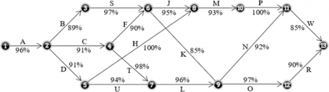
Example: A project proceeds according to specific plans to accomplish it in the best possible way, as shown in the graph of its network in Figure 2. According to those plans, the project is accomplished through the completion of its activities that lead to the completion of all its events. Accordingly, Table 1 includes the cost and the quality percentage for each activity carried out in the project when working in the normal situation and when working in the quality maximization situation. In this regard, the project management seeks to optimizing the overall quality of the project after its completion by making it to be at least 94% in exchange for the least additional costs allocated to resources through which the quality optimization process is carried out.
Table 1. Project network data
|
Activities |
Normal |
Optimize |
||
|
Quality (Percent) |
Cost (€) |
Quality (Percent) |
Cost (€) |
|
|
❶─A➝❷ |
96 |
9160 |
100 |
9800 |
|
❷─B➝❸ |
89 |
7840 |
100 |
9600 |
|
❷─C➝❹ |
91 |
8328 |
100 |
9750 |
|
❷─D➝❺ |
91 |
8223 |
100 |
9600 |
|
❸─S➝❻ |
97 |
8905 |
100 |
9400 |
|
❹─F➝❻ |
90 |
7750 |
100 |
9300 |
|
❹─T➝❼ |
98 |
9380 |
100 |
9700 |
|
❺─U─❼ |
94 |
8656 |
100 |
9640 |
|
❺─H➝❽ |
100 |
8800 |
100 |
8800 |
|
❻─J➝❽ |
95 |
8570 |
100 |
9400 |
|
❻─K─❾ |
85 |
7050 |
100 |
9300 |
|
❼─L➝❾ |
96 |
8460 |
100 |
9100 |
|
❽─M➝❿ |
93 |
7815 |
100 |
8900 |
|
❾─N➝⓫ |
92 |
7880 |
100 |
9200 |
|
❾─O➝⓬ |
97 |
9035 |
100 |
9500 |
|
❿─P➝⓫ |
100 |
8800 |
100 |
8800 |
|
⓫─W➝⓭ |
85 |
7620 |
100 |
9900 |
|
⓬─R➝⓭ |
90 |
8230 |
100 |
9800 |
Solution: It is known that the basis of the work of all algorithms depends on their inputs to obtain their outputs, and in this regard the STQO inputs of this problem must first be defined. It is clear that all the project data required by inputs have been mentioned in Table 1. While the project network graph has been given in this example as shown in Figure 2 which includes 13 vertices (events) and 18 edges (activity). Now STQO will start working from the step 1 in the phase 1 until obtaining outputs after implementing step 6 in the phase 2 of this algorithm. The step 1 is to calculate the value of the quality optimization cost slope $S_{ij}$ for each unit in all project activities, which is stated in Table 2 in order to write the objective function according to formula (4).
Table 2. The quality optimization cost slope per unit at all activities
|
Activities |
Normal |
Optimization |
∆ |
$S_{i j}$ (€) |
|||
|
Quality (Percent) |
Cost (€) |
Quality (Percent) |
Cost (€) |
$\Delta \boldsymbol{Q}_{i j}$ (Percent) |
$\Delta C_{i j}$ (€) |
||
|
❶─A➝❷ |
96 |
9160 |
100 |
9800 |
4 |
640 |
160 |
|
❷─B➝❸ |
89 |
7840 |
100 |
9600 |
11 |
1760 |
160 |
|
❷─C➝❹ |
91 |
8328 |
100 |
9750 |
9 |
1422 |
158 |
|
❷─D➝❺ |
91 |
8223 |
100 |
9600 |
9 |
1377 |
153 |
|
❸─S➝❻ |
97 |
8905 |
100 |
9400 |
3 |
495 |
165 |
|
❹─F➝❻ |
90 |
7750 |
100 |
9300 |
10 |
1550 |
155 |
|
❹─T➝❼ |
98 |
9380 |
100 |
9700 |
2 |
320 |
160 |
|
❺─U─❼ |
94 |
8656 |
100 |
9640 |
6 |
984 |
164 |
|
❺─H➝❽ |
100 |
8800 |
100 |
8800 |
0 |
0 |
- |
|
❻─J➝❽ |
95 |
8570 |
100 |
9400 |
5 |
830 |
166 |
|
❻─K─❾ |
85 |
7050 |
100 |
9300 |
15 |
2250 |
150 |
|
❼─L➝❾ |
96 |
8460 |
100 |
9100 |
4 |
640 |
160 |
|
❽─M➝❿ |
93 |
7815 |
100 |
8900 |
7 |
1085 |
155 |
|
❾─N➝⓫ |
92 |
7880 |
100 |
9200 |
8 |
1320 |
165 |
|
❾─O➝⓬ |
97 |
9035 |
100 |
9500 |
3 |
465 |
155 |
|
❿─P➝⓫ |
100 |
8800 |
100 |
8800 |
0 |
0 |
- |
|
⓫─W➝⓭ |
85 |
7620 |
100 |
9900 |
15 |
2280 |
152 |
|
⓬─R➝⓭ |
90 |
8230 |
100 |
9800 |
10 |
1570 |
157 |
After that, based on the project network graph, all paths in $Ps$ that form that graph will be drawn below, which begin with the initial vertex numbered ❶ and end with the final vertex numbered ⓭, in order to write the set of constraints for all those paths according to formula (6).
Figure 2. The graph $G$ of the project network in the above example
Path 1: ❶─A➝❷─B➝❸─S➝❻─J➝❽─M➝❿─P➝⓫─W➝⓭
Path 2: ❶─A➝❷─B➝❸─S➝❻─K➝❾─N➝⓫─W➝⓭
Path 3: ❶─A➝❷─B➝❸─S➝❻─K➝❾─O➝⓬─R➝⓭
Path 4: ❶─A➝❷─C➝❹─F➝❻─J➝❽─M➝❿─P➝⓫─W➝⓭
Path 5: ❶─A➝❷─C➝❹─F➝❻─K➝❾─N➝⓫─W➝⓭
Path 6: ❶─A➝❷─C➝❹─F➝❻─K➝❾─O➝⓬─R➝⓭
Path 7: ❶─A➝❷─C➝❹─T➝❼─U➝❺─H➝❽─M➝❿─P➝⓫─W➝⓭
Path 8: ❶─A➝❷─C➝❹─T➝❼─L➝❾─K➝❻─J➝❽─M➝❿─P➝⓫─W➝⓭
Path 9: ❶─A➝❷─C➝❹─T➝❼─L➝❾─N➝⓫─W➝⓭
Path 10: ❶─A➝❷─C➝❹─T➝❼─L➝❾─O➝⓬─R➝⓭
Path 11: ❶─A➝❷─D➝❺─H➝❽─M➝❿─P➝⓫─W➝⓭
Path 12: ❶─A➝❷─D➝❺─U➝❼─L➝❾─K➝❻─J➝❽─M➝❿─P➝⓫─W➝⓭
Path 13: ❶─A➝❷─D➝❺─U➝❼─L➝❾─N➝⓫─W➝⓭
Path 14: ❶─A➝❷─D➝❺─U➝❼─L➝❾─O➝⓬─R➝⓭
Thus, the mathematical model of the problem mentioned in this example can be built according to formulas from (4) to (7) after defining decision variables with the following hypothesis. Assume that:
$x_{1\,\,2}$ is the amount of increase when optimizing the quality of activity A.
$x_{2\,\,3}$ is the amount of increase when optimizing the quality of activity B.
$x_{2\,\,4}$ is the amount of increase when optimizing the quality of activity C.
$x_{2\,\,5}$ is the amount of increase when optimizing the quality of activity D.
$x_{3\,\,6}$ is the amount of increase when optimizing the quality of activity S.
$x_{4\,\,6}$ is the amount of increase when optimizing the quality of activity F.
$x_{4\,\,7}$ is the amount of increase when optimizing the quality of activity T.
$x_{5\,\,7}$ is the amount of increase when optimizing the quality of activity U.
$x_{5\,\,8}$ is the amount of increase when optimizing the quality of activity H.
$x_{6\,\,8}$ is the amount of increase when optimizing the quality of activity J.
$x_{6\,\,9}$ is the amount of increase when optimizing the quality of activity K.
$x_{7\,\,9}$ is the amount of increase when optimizing the quality of activity L.
$x_{8\,\,10}$ is the amount of increase when optimizing the quality of activity M.
$x_{9\,\,11}$ is the amount of increase when optimizing the quality of activity N.
$x_{9\,\,12}$ is the amount of increase when optimizing the quality of activity O.
$x_{10\,\, 11}$ is the amount of increase when optimizing the quality of activity P.
$x_{11\,\, 13}$ is the amount of increase when optimizing the quality of activity W.
$x_{12\,\, 13}$ is the amount of increase when optimizing the quality of activity R.
Objective function
$\begin{aligned} \min f(x)= & 160 x_{1\,\, 2}+160 x_{2\,\, 3}+158 x_{2\,\, 4}+153 x_{2\,\, 5} \\ & +165 x_{3\,\, 6}+155 x_{4\,\, 6}+160 x_{4\,\, 7}+164 x_{5\,\, 7} \\ & +166 x_{6\,\, 8}+150 x_{6\,\, 9}+160 x_{7\,\, 9} \\ & +155 x_{8\,\, 10}+165 x_{9\,\, 11}+155 x_{9\,\, 12} \\ & +152 x_{11\,\, 13}+157 x_{12\,\, 13}\end{aligned}$
Subject to
Constraints of increasing quality for each activity:
$\begin{gathered}x_{1\,\, 2} \leq 4 \%, x_{2\,\, 3} \leq 11 \%, x_{2\,\, 4} \leq 9 \%, x_{2\,\, 5} \leq 9 \%, x_{3\,\, 6} \leq 3 \% \\ x_{4\,\, 6} \leq 10 \%, x_{4\,\, 7} \leq 2 \%, x_{5\,\, 7} \leq 6 \%, x_{5\,\, 8}=0 \%, x_{6\,\, 8} \leq 5 \% \\ x_{6\,\, 9} \leq 15 \%, x_{7\,\, 9} \leq 4 \%, x_{8\,\, 10} \leq 7 \%, x_{9\,\, 11} \leq 8 \%, x_{9\,\, 12} \leq 3 \% \\ x_{10\,\, 11}=0 \%, x_{11\,\, 13} \leq 15 \%, x_{12\,\, 13} \leq 10 \%\end{gathered}$
Constraints of graph paths:
$\begin{gathered}\frac{96 \%+x_{1\,\, 2}+89 \%+x_{2\,\, 3}+97 \%+x_{3\,\, 6}+95 \%+x_{6\,\, 8}+93 \%+x_{8\,\, 10}+100 \%+x_{10\,\, 11}+85 \%+x_{11\,\, 13}}{7} \geq 94 \% \\ \Rightarrow x_{1\,\, 2}+x_{2\,\, 3}+x_{3\,\, 6}+x_{6\,\, 8}+x_{8\,\, 10}+x_{10\,\, 11}+x_{11\,\, 13} \geq 3 \% \\ \frac{96 \%+x_{1\,\, 2}+89 \%+x_{2\,\, 3}+97 \%+x_{3\,\, 6}+85 \%+x_{6\,\, 9}+92 \%+x_{9\,\, 11}+85 \%+x_{11\,\, 13}}{6} \geq 94 \% \\ \Rightarrow x_{1\,\, 2}+x_{2\,\, 3}+x_{3\,\, 6}+x_{6\,\, 9}+x_{9\,\, 11}+x_{11\,\, 13} \geq 20 \% \\ \frac{96 \%+x_{1\,\, 2}+89 \%+x_{2\,\, 3}+97 \%+x_{3\,\, 6}+85 \%+x_{6\,\, 9}+97 \%+x_{9\,\, 12}+90 \%+x_{12\,\, 13}}{6} \geq 94 \% \\ \Rightarrow x_{1\,\, 2}+x_{2\,\, 3}+x_{3\,\, 6}+x_{6\,\, 9}+x_{9\,\, 12}+x_{12\,\, 13} \geq 10 \% \\ \frac{96 \%+x_{1\,\, 2}+91 \%+x_{2\,\, 4}+90 \%+x_{4\,\, 6}+95 \%+x_{6\,\, 8}+93 \%+x_{8\,\, 10}+100 \%+x_{10\,\, 11}+85 \%+x_{11\,\, 13}}{7} \geq 94 \% \\ \Rightarrow x_{1\,\, 2}+x_{2\,\, 4}+x_{4\,\, 6}+x_{6\,\, 8}+x_{8\,\, 10}+x_{10\,\, 11}+x_{11\,\, 13} \geq 8 \%\end{gathered}$
$\begin{gathered}\frac{96 \%+x_{1\,\, 2}+91 \%+x_{2\,\, 4}+90 \%+x_{4\,\, 6}+85 \%+x_{6\,\, 9}+92 \%+x_{9\,\, 11}+85 \%+x_{11\,\, 13}}{6} \geq 94 \% \\ \Rightarrow x_{1\,\, 2}+x_{2\,\, 4}+x_{4\,\, 6}+x_{6\,\, 9}+x_{9\,\, 11}+x_{11\,\, 13} \geq 25 \% \\ \frac{96 \%+x_{1\,\, 2}+91 \%+x_{2\,\, 4}+90 \%+x_{4\,\, 6}+85 \%+x_{6\,\, 9}+97 \%+x_{9\,\, 12}+90 \%+x_{12\,\, 13}}{6} \geq 94 \% \\ \Rightarrow x_{1\,\, 2}+x_{2\,\, 4}+x_{4\,\, 6}+x_{6\,\, 9}+x_{9\,\, 12}+x_{12\,\, 13} \geq 15 \% \\ \frac{96 \%+x_{1\,\, 2}+91 \%+x_{2\,\, 4}+98 \%+x_{4\,\, 7}+94 \%+x_{7\,\, 5}+100 \%+x_{5\,\, 8}+93 \%+x_{8\,\, 10}+100 \%+x_{10\,\, 11}+85 \%+x_{11\,\, 13}}{8} \\ \geq 94 \% \Rightarrow x_{1\,\, 2}+x_{2\,\, 4}+x_{4\,\, 7}+x_{7\,\, 5}+x_{5\,\, 8}+x_{8\,\, 10}+x_{10\,\, 11}+x_{11\,\, 13} \geq-5 \% \\ \frac{96 \%+x_{1\,\, 2}+91 \%+x_{2\,\, 4}+98 \%+x_{4\,\, 7}+96 \%+x_{7\,\, 9}+85 \%+x_{9\,\, 6}+95 \%+x_{6\,\, 8}+93 \%+x_{8\,\, 10}+100 \%+x_{10\,\, 11}+85 \%+x_{11\,\, 13}}{9} \\ \geq 94 \% \Rightarrow x_{1\,\, 2}+x_{2\,\, 4}+x_{4\,\, 7}+x_{7\,\, 9}+x_{9\,\, 6}+x_{6\,\, 8}+x_{8\,\, 10}+x_{10\,\, 11}+x_{11\,\, 13} \geq 7 \%\end{gathered}$
$\begin{aligned} & \frac{96 \%+x_{1\,\, 2}+91 \%+x_{2\,\, 4}+98 \%+x_{4\,\, 7}+96 \%+x_{7\,\, 9}+92 \%+x_{9\,\, 11}+85 \%+x_{11\,\, 13}}{6} \geq 94 \% \\ & \quad \Rightarrow x_{1\,\, 2}+x_{2\,\, 4}+x_{4\,\, 7}+x_{7\,\, 9}+x_{9\,\, 11}+x_{11\,\, 13} \geq 6 \% \\ & \frac{96 \%+x_{1\,\, 2}+91 \%+x_{2\,\, 4}+98 \%+x_{4\,\, 7}+96 \%+x_{7\,\, 9}+97 \%+x_{9\,\, 12}+90 \%+x_{12\,\, 13}}{6} \geq 94 \% \\ & \quad \Rightarrow x_{1\,\, 2}+x_{2\,\, 4}+x_{4\,\, 7}+x_{7\,\, 9}+x_{9\,\, 12}+x_{12\,\, 13} \geq-4 \% \\ & \frac{96 \%+x_{1\,\, 2}+91 \%+x_{2\,\, 5}+100 \%+x_{5\,\, 8}+93 \%+x_{8\,\, 10}+100 \%+x_{10\,\, 11}+85 \%+x_{11\,\, 13}}{6} \geq 94 \% \\ & \Rightarrow x_{1\,\, 2}+x_{2\,\, 5}+x_{5\,\, 8}+x_{8\,\, 10}+x_{10\,\, 11}+x_{11\,\, 13} \geq-1 \%\end{aligned}$
$\begin{gathered}\frac{96 \%+x_{1\,\, 2}+91 \%+x_{2\,\, 5}+94 \%+x_{5\,\, 7}+96 \%+x_{7\,\, 9}+85 \%+x_{9\,\, 6}+95 \%+x_{6\,\, 8}+93 \%+x_{8\,\, 10}+100 \%+x_{10\,\, 11}+85 \%+x_{11\,\, 13}}{9} \\ \geq 94 \% \Rightarrow x_{1\,\, 2}+x_{2\,\, 5}+x_{5\,\, 7}+x_{7\,\, 9}+x_{9\,\, 6}+x_{6\,\, 8}+x_{8\,\, 10}+x_{10\,\, 11}+x_{11\,\, 13} \geq 11 \% \\ \frac{96 \%+x_{1\,\, 2}+91 \%+x_{2\,\, 5}+94 \%+x_{5\,\, 7}+96 \%+x_{7\,\, 9}+92 \%+x_{9\,\, 11}+85 \%+x_{11\,\, 13}}{6} \geq 94 \% \\ \Rightarrow x_{1\,\, 2}+x_{2\,\, 5}+x_{5\,\, 7}+x_{7\,\, 9}+x_{9\,\, 11}+x_{11\,\, 13} \geq 10 \% \\ \frac{96 \%+x_{1\,\, 2}+91 \%+x_{2\,\, 5}+94 \%+x_{5\,\, 7}+96 \%+x_{7\,\, 9}+97 \%+x_{9\,\, 12}+90 \%+x_{12\,\, 13}}{6} \geq 94 \% \\ \Rightarrow x_{1\,\, 2}+x_{2\,\, 5}+x_{5\,\, 7}+x_{7\,\, 9}+x_{9\,\, 12}+x_{12\,\, 13} \geq 0 \%\end{gathered}$
Constraints of non-negativity.
$x_{i j} \geq 0, \forall i, j$ and $i \neq j$ where $i=1,2, \ldots, 12$ but $j=2$, $3, \ldots, 13$.
Based on the above, the phase 1 of the STQO algorithm work ended after the completion of building the above mathematical model. After that, the phase 2 of the STQO algorithm started working and its implementation in the Microsoft Excel program for the purpose of using the “Solver” tool. In order to clarify some of happenings of this phase, Table 3 was presented, which included writing the mathematical model for this problem in the Microsoft Excel program and the appearance of the result of the objective function after implementing the “Solver” tool.
Now STQO outputs are obtained to solve the problem given in this example as follows.
Table 3. Mathematical model of the problem in the Microsoft Excel
|
Variables |
XA |
XB |
XC |
XD |
XS |
XF |
XT |
XU |
XH |
XJ |
XK |
XL |
XM |
XN |
XO |
XP |
XW |
XR |
Total |
Relation |
R.H.S. |
|
Objective |
|
|
|
|
|
|
|
|
|
|
|
|
|
|
|
|
|
|
|
|
|
|
Coefficients |
160 |
160 |
158 |
153 |
165 |
155 |
160 |
164 |
0 |
166 |
150 |
160 |
155 |
165 |
155 |
0 |
152 |
157 |
|
|
|
|
Values |
0 |
0 |
0 |
0 |
0 |
0 |
0 |
0 |
0 |
0 |
15 |
0 |
0 |
0 |
0 |
0 |
10 |
0 |
3770 |
|
|
|
Constraints |
|
|
|
|
|
|
|
|
|
|
|
|
|
|
|
|
|
|
|
|
|
|
Cons. (1) |
1 |
0 |
0 |
0 |
0 |
0 |
0 |
0 |
0 |
0 |
0 |
0 |
0 |
0 |
0 |
0 |
0 |
0 |
0 |
≤ |
4 |
|
Cons. (2) |
0 |
1 |
0 |
0 |
0 |
0 |
0 |
0 |
0 |
0 |
0 |
0 |
0 |
0 |
0 |
0 |
0 |
0 |
0 |
≤ |
11 |
|
Cons. (3) |
0 |
0 |
1 |
0 |
0 |
0 |
0 |
0 |
0 |
0 |
0 |
0 |
0 |
0 |
0 |
0 |
0 |
0 |
0 |
≤ |
9 |
|
Cons. (4) |
0 |
0 |
0 |
1 |
0 |
0 |
0 |
0 |
0 |
0 |
0 |
0 |
0 |
0 |
0 |
0 |
0 |
0 |
0 |
≤ |
9 |
|
Cons. (5) |
0 |
0 |
0 |
0 |
1 |
0 |
0 |
0 |
0 |
0 |
0 |
0 |
0 |
0 |
0 |
0 |
0 |
0 |
0 |
≤ |
3 |
|
Cons. (6) |
0 |
0 |
0 |
0 |
0 |
1 |
0 |
0 |
0 |
0 |
0 |
0 |
0 |
0 |
0 |
0 |
0 |
0 |
0 |
≤ |
10 |
|
Cons. (7) |
0 |
0 |
0 |
0 |
0 |
0 |
1 |
0 |
0 |
0 |
0 |
0 |
0 |
0 |
0 |
0 |
0 |
0 |
0 |
≤ |
2 |
|
Cons. (8) |
0 |
0 |
0 |
0 |
0 |
0 |
0 |
1 |
0 |
0 |
0 |
0 |
0 |
0 |
0 |
0 |
0 |
0 |
0 |
≤ |
6 |
|
Cons. (9) |
0 |
0 |
0 |
0 |
0 |
0 |
0 |
0 |
1 |
0 |
0 |
0 |
0 |
0 |
0 |
0 |
0 |
0 |
0 |
= |
0 |
|
Cons. (10) |
0 |
0 |
0 |
0 |
0 |
0 |
0 |
0 |
0 |
1 |
0 |
0 |
0 |
0 |
0 |
0 |
0 |
0 |
0 |
≤ |
5 |
|
Cons. (11) |
0 |
0 |
0 |
0 |
0 |
0 |
0 |
0 |
0 |
0 |
1 |
0 |
0 |
0 |
0 |
0 |
0 |
0 |
15 |
≤ |
15 |
|
Cons. (12) |
0 |
0 |
0 |
0 |
0 |
0 |
0 |
0 |
0 |
0 |
0 |
1 |
0 |
0 |
0 |
0 |
0 |
0 |
0 |
≤ |
4 |
|
Cons. (13) |
0 |
0 |
0 |
0 |
0 |
0 |
0 |
0 |
0 |
0 |
0 |
0 |
1 |
0 |
0 |
0 |
0 |
0 |
0 |
≤ |
7 |
|
Cons. (14) |
0 |
0 |
0 |
0 |
0 |
0 |
0 |
0 |
0 |
0 |
0 |
0 |
0 |
1 |
0 |
0 |
0 |
0 |
0 |
≤ |
8 |
|
Cons. (15) |
0 |
0 |
0 |
0 |
0 |
0 |
0 |
0 |
0 |
0 |
0 |
0 |
0 |
0 |
1 |
0 |
0 |
0 |
0 |
≤ |
3 |
|
Cons. (16) |
0 |
0 |
0 |
0 |
0 |
0 |
0 |
0 |
0 |
0 |
0 |
0 |
0 |
0 |
0 |
1 |
0 |
0 |
0 |
= |
0 |
|
Cons. (17) |
0 |
0 |
0 |
0 |
0 |
0 |
0 |
0 |
0 |
0 |
0 |
0 |
0 |
0 |
0 |
0 |
1 |
0 |
10 |
≤ |
15 |
|
Cons. (18) |
0 |
0 |
0 |
0 |
0 |
0 |
0 |
0 |
0 |
0 |
0 |
0 |
0 |
0 |
0 |
0 |
0 |
1 |
0 |
≤ |
10 |
|
Cons. (19) |
1 |
1 |
0 |
0 |
1 |
0 |
0 |
0 |
0 |
1 |
0 |
0 |
1 |
0 |
0 |
1 |
1 |
0 |
10 |
≥ |
3 |
|
Cons. (20) |
1 |
1 |
0 |
0 |
1 |
0 |
0 |
0 |
0 |
0 |
1 |
0 |
0 |
1 |
0 |
0 |
1 |
0 |
25 |
≥ |
20 |
|
Cons. (21) |
1 |
1 |
0 |
0 |
1 |
0 |
0 |
0 |
0 |
0 |
1 |
0 |
0 |
0 |
1 |
0 |
0 |
1 |
15 |
≥ |
10 |
|
Cons. (22) |
1 |
0 |
1 |
0 |
0 |
1 |
0 |
0 |
0 |
1 |
0 |
0 |
1 |
0 |
0 |
1 |
1 |
0 |
10 |
≥ |
8 |
|
Cons. (23) |
1 |
0 |
1 |
0 |
0 |
1 |
0 |
0 |
0 |
0 |
1 |
0 |
0 |
1 |
0 |
0 |
1 |
0 |
25 |
≥ |
25 |
|
Cons. (24) |
1 |
0 |
1 |
0 |
0 |
1 |
0 |
0 |
0 |
0 |
1 |
0 |
0 |
0 |
1 |
0 |
0 |
1 |
15 |
≥ |
15 |
|
Cons. (25) |
1 |
0 |
1 |
0 |
0 |
0 |
1 |
1 |
1 |
0 |
0 |
0 |
1 |
0 |
0 |
1 |
1 |
0 |
10 |
≥ |
-5 |
|
Cons. (26) |
1 |
0 |
1 |
0 |
0 |
0 |
1 |
0 |
0 |
1 |
1 |
1 |
1 |
0 |
0 |
1 |
1 |
0 |
25 |
≥ |
7 |
|
Cons. (27) |
1 |
0 |
1 |
0 |
0 |
0 |
1 |
0 |
0 |
0 |
0 |
1 |
0 |
1 |
0 |
0 |
1 |
0 |
10 |
≥ |
6 |
|
Cons. (28) |
1 |
0 |
1 |
0 |
0 |
0 |
1 |
0 |
0 |
0 |
0 |
1 |
0 |
0 |
1 |
0 |
0 |
1 |
0 |
≥ |
-4 |
|
Cons. (29) |
1 |
0 |
0 |
1 |
0 |
0 |
0 |
0 |
1 |
0 |
0 |
0 |
1 |
0 |
0 |
1 |
1 |
0 |
10 |
≥ |
-1 |
|
Cons. (30) |
1 |
0 |
0 |
1 |
0 |
0 |
0 |
1 |
0 |
1 |
1 |
1 |
1 |
0 |
0 |
1 |
1 |
0 |
25 |
≥ |
11 |
|
Cons. (31) |
1 |
0 |
0 |
1 |
0 |
0 |
0 |
1 |
0 |
0 |
0 |
1 |
0 |
1 |
0 |
0 |
1 |
0 |
10 |
≥ |
10 |
|
Cons. (32) |
1 |
0 |
0 |
1 |
0 |
0 |
0 |
1 |
0 |
0 |
0 |
1 |
0 |
0 |
1 |
0 |
0 |
1 |
0 |
≥ |
0 |
This section will discuss and analyze results of the previous section in particular after discussing what was presented in this paper in general. Before starting that, it is necessary to point out the most important thing that was dealt with in this study in general, which is the formulation of the new mathematical model that simulates the quality-cost trade-off problem firstly, and then the design of STQO to solve this problem secondly. Among what was discussed in this section are most prominent reasons that led to the distinction of this new model and the vantage of STQO in terms of performance and results. One of reasons that led to the efficiency of the new mathematical model presented in this paper lies in converting the project network into a graph. Based on this graph, all paths that form it are determined, starting from the first vertex (the initial event) and ending at the last vertex (the final event). In this regard, the reason for specifying all paths which form that graph is the lack of knowledge of working conditions on any specific path that necessitate the progress of the project’s completion. For your information, when per path of these paths is followed individually, the project is completed, but at varying costs from one path to another. Hence, the fruit of this appears through the formulation of the most important set of constraints, as shown in formula (6) above, to which the objective function must be subjected in that new mathematical model to improve the overall quality at lowest additional costs. After reading the STQO algorithm, it is expected that the reader will wonder why this algorithm was divided into two phases! STQO is a technique that uses a linear programming approach represented by the simplex method in order to solve the quality-cost trade-off problem. Therefore, this matter requires formulating the problem with a mathematical model firstly in order to use the simplex method secondly, which makes the STQO algorithm consist of a theoretical phase followed by a practical phase. From this principle, the role of the theoretical phase is highlighted through preparing the mathematical model for the problem in question, which requires focusing and looking deeply into the problem in order to formulate it mathematically according to the new mathematical model included in this study. After that, the second phase can be implemented, which is the practical phase that requires the presence of that model. The second phase is to work on using the “Solver” tool in the Microsoft Excel to obtain the final solution by using the simplex method. The reason for using the “Solver” tool is that it provides a lot of effort and time in performing calculations required by the simplex method, and this tool is also characterized by ease of use. There is no doubt that STQO’s excellence in using the “Solver” tool made it highly efficient in its performance, in addition to its choice of the simplex method for the solution, which enabled it to be trustworthy in terms of its numerical results.
In fact, it is clear from the problem mentioned in the previous example that the number of decision variables in it is 18 variables, through which the mathematical model for that problem is built. This number is related to the number of edges (activities) of the project network graph. While the number of constraints to which the objective function was subjected is 32 constraints (without the non-negativity constraint), with 18 constraints representing constraints of the permissible increase in quality for each activity, in addition to 14 constraints representing paths constraints that form the project network graph. It is worth noting to point out what the sign of the constant value of the right side in each path constraint means after making it in its simplest form, which starts from constraint (19) and ends with constraint (32). In particular, if the value of the right side of any of these constraints is a positive sign, this means that the quality of the path which has that constraint is less than the overall quality specified by the project management. Whereas if the value of this right side of one of constraints is a negative sign, it means that the quality of the path which has that constraint is greater than the overall quality specified previously. But if the value of that right side in a specific constraint is zero, this indicates that the quality of the path that has this specific constraint is equal to the overall quality required for the project. Note that what was discussed above is useful in guessing proceedings of action of the second phase of STQO algorithm. The second phase of the STQO algorithm was implemented to solve the problem in the example above by using the “Solver” tool in the Microsoft Excel program installed in a laptop computer manufactured by Acer. This laptop is from type a 3rd generation Intel® CoreTM i3 with a speed of 2.5GHz, and the RAM size is 4 GB DDR3 Memory, while the hard disk size is 500 GB HDD. In general, one of the most important things in the performance of algorithms is the time it takes to solve problems for which they were designed. In particular, the time it took to execute the second phase of the STQO algorithm in solving this problem was 0.016 seconds on that laptop. Meanwhile, the number of iterations of the solution was 17 iterations by using the simplex method, which was used to solve this problem with the “Solver” tool. Furthermore, you can see the remaining details of the solution shown in Table 4, which represents the answer report after completing the implementation of the “Solver” tool in the Microsoft Excel program.
Table 4. The answer report after implementing the “Solver” tool
|
|
|
|
|
|
|
Microsoft Excel 14.0 Answer Report |
|
|
|
|
|
|
|
Worksheet: [Solver Application to Solve Example 2 - للإطروحة والبحث5.xlsx]ورقة1 |
|
|
|
|
|
|
|
Result: Solver found a solution. All Constraints and optimality conditions are satisfied. |
|
|
|
|
|
|
|
Solver Engine |
|
|
|
|
|
|
Engine: Simplex LP |
|
|
|
|
|
|
|
Solution Time: 0.016 Seconds. |
|
|
|
|
|
|
|
Iterations: 17 Subproblems: 0 |
|
|
|
|
|
|
|
|
Solver Options |
|
|
|
|
|
|
Max Time Unlimited, Iterations Unlimited, Precision 0.000001, Use Automatic Scaling |
|
|
|
|
|
|
|
Max Subproblems Unlimited, Max Integer Sols Unlimited, Integer Tolerance 1%, Solve Without Integer Constraints, Assume Nonnegative |
|
|
Table 4(a) |
|
|
|
|
Objective Cell (Min) |
|
|
|
|
Final Value |
Original Value |
Name |
Cell |
|
|
|
|
D6 |
Total |
0 |
3770 |
|
|
Table 4(b) |
|
|
|
|
Variable Cells |
|
|
|
Integer |
Final Value |
Original Value |
Name |
Cell |
|
|
|
Integer |
0 |
0 |
XR |
E6 |
|
|
|
Integer |
10 |
0 |
XW |
F6 |
|
|
|
Integer |
0 |
0 |
XP |
G6 |
|
|
|
Integer |
0 |
0 |
XO |
H6 |
|
|
|
Integer |
0 |
0 |
XN |
I6 |
|
|
|
Integer |
0 |
0 |
XM |
J6 |
|
|
|
Integer |
0 |
0 |
XL |
K6 |
|
|
|
Integer |
15 |
0 |
XK |
L6 |
|
|
|
Integer |
0 |
0 |
XJ |
M6 |
|
|
|
Integer |
0 |
0 |
XH |
N6 |
|
|
|
Integer |
0 |
0 |
XU |
O6 |
|
|
|
Integer |
0 |
0 |
XT |
P6 |
|
|
|
Integer |
0 |
0 |
XF |
Q6 |
|
|
|
Integer |
0 |
0 |
XS |
R6 |
|
|
|
Integer |
0 |
0 |
XD |
S6 |
|
|
|
Integer |
0 |
0 |
XC |
T6 |
|
|
|
Integer |
0 |
0 |
XB |
U6 |
|
|
|
Integer |
0 |
0 |
XA |
V6 |
|
|
Table 4(c) |
|
|
|
|
Constraints |
|
|
Slack |
Status |
Formula |
Cell Value |
Name |
Cell |
|
|
0 |
Binding |
D17=B17 |
0 |
= Total |
D17 |
|
|
5 |
Not Binding |
D18<=B18 |
0 |
≤ Total |
D18 |
|
|
0 |
Binding |
D19<=B19 |
15 |
≤ Total |
D19 |
|
|
4 |
Not Binding |
D20<=B20 |
0 |
≤ Total |
D20 |
|
|
7 |
Not Binding |
D21<=B21 |
0 |
≤ Total |
D21 |
|
|
8 |
Not Binding |
D22<=B22 |
0 |
≤ Total |
D22 |
|
|
3 |
Not Binding |
D23<=B23 |
0 |
≤ Total |
D23 |
|
|
0 |
Binding |
D24=B24 |
0 |
= Total |
D24 |
|
|
5 |
Not Binding |
D25<=B25 |
10 |
≤ Total |
D25 |
|
|
10 |
Not Binding |
D26<=B26 |
0 |
≤ Total |
D26 |
|
|
7 |
Not Binding |
D27>=B27 |
10 |
≥ Total |
D27 |
|
|
5 |
Not Binding |
D28>=B28 |
25 |
≥ Total |
D28 |
|
|
5 |
Not Binding |
D29>=B29 |
15 |
≥ Total |
D29 |
|
|
2 |
Not Binding |
D30>=B30 |
10 |
≥ Total |
D30 |
|
|
0 |
Binding |
D31>=B31 |
25 |
≥ Total |
D31 |
|
|
0 |
Binding |
D32>=B32 |
15 |
≥ Total |
D32 |
|
|
15 |
Not Binding |
D33>=B33 |
10 |
≥ Total |
D33 |
|
|
18 |
Not Binding |
D34>=B34 |
25 |
≥ Total |
D34 |
|
|
4 |
Not Binding |
D35>=B35 |
10 |
≥ Total |
D35 |
|
|
4 |
Not Binding |
D36>=B36 |
0 |
≥ Total |
D36 |
|
|
11 |
Not Binding |
D37>=B37 |
10 |
≥ Total |
D37 |
|
|
14 |
Not Binding |
D38>=B38 |
25 |
≥ Total |
D38 |
|
|
0 |
Binding |
D39>=B39 |
10 |
≥ Total |
D39 |
|
|
0 |
Binding |
D40>=B40 |
0 |
≥ Total |
D40 |
|
|
4 |
Not Binding |
D9<=B9 |
0 |
≤ Total |
D9 |
|
|
11 |
Not Binding |
D10<=B10 |
0 |
≤ Total |
D10 |
|
|
9 |
Not Binding |
D11<=B11 |
0 |
≤ Total |
D11 |
|
|
9 |
Not Binding |
D12<=B12 |
0 |
≤ Total |
D12 |
|
|
3 |
Not Binding |
D13<=B13 |
0 |
≤ Total |
D13 |
|
|
10 |
Not Binding |
D14<=B14 |
0 |
≤ Total |
D14 |
|
|
2 |
Not Binding |
D15<=B15 |
0 |
≤ Total |
D15 |
|
|
6 |
Not Binding |
D16<=B16 |
0 |
≤ Total |
D16 |
|
|
|
|
|
|
|
E6:V6=Integer |
|
It is noted in Table 4 that there are three tables, which are very important because they show the result in a detailed and clearer manner. The Table 4(a) is for the value of the objective function, the Table 4(b) is for values of decision variables, while the Table 4(c) shows the state of constraints in terms of the amount of satisfaction, so it is called the constraint saturation table. In the Table 3, it is noted that there is a difference in terms of saturation of constraints. The reason is that these constraints include the dissimilarity sign with equality (≥,≤), as in the general formula of the new mathematical model, and not just equality (=). Hence the work of the simplex method, as known, is to achieve the objective function while being subject to all constraints, regardless of whether constraints are saturated or not if they are with one of signs of inequality. Based on this, lies the following conclusion in general, which is that STQO is concerned in solving the quality-cost trade-off problem within the required overall quality only and not more for the project or product when it is completed. And this is of very great importance in reducing additional costs required by the quality optimization process.
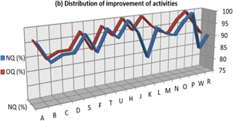
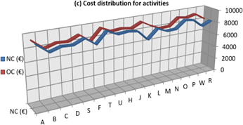
In order to discuss results in a more precise, it is necessary to explain the fundamental reason for the value of the decision variable $x_{6\,\,9}=15 \%$, which led to the complete saturation of constraint (11). While the value of the decision variable $x_{11\,\,13}=10 \%$ did not lead to the complete saturation of constraint (17). Why wasn't it the other way around in that case? Certainly, the reason for the above lies in the fact that the value of $S_{6\,\,9}=150 €$ for $x_{6\,\,9}$ is less than the value of $S_{11\,\,13}=152 €$ for $x_{11\,\,13}$ as this appears in Table 2. Accordingly, this means that the cost of increasing the quality per unit of activity K is less than the cost of increasing the quality per unit of activity W. Therefore, meeting constraint (11) to the saturation limit is more important than meeting constraint (17) to the saturation limit. Because, according to the above, constraint (11) has a better effect on the final result. Depending on this, the quality of activity K was improved from 85% to 100%, while activity W was improved from 85% to 95% and no more. The reason lies in the fact that this new value for the quality of activity W after optimization represents the lowest possible value to meet the overall quality required for the project, and it was sufficient and not more, with the aim of not incurring more additional costs. Thus, without the slightest doubt, the reason is clear why values of the zero and non-zero decision variables became like this, which in turn achieved the objective function at its best value while being subject to constraints imposed on it. Therefore, results obtained by solving the mathematical model of the problem mentioned in the previous section indicate that the overall quality of the project can be optimized to at least 94%, in exchange for 3770 €, which is the added cost for the process of optimizing the overall quality. In particular, Table 5 has been created below to show results of the problem presented in the previous section more accurately and clearly. Also, below in Figure 3 were drawn diagrams that show the distribution of the cost slope $S_{ij}$ for all project activities as in Figure 3(a) and the distribution of improvement for all these activities shown in Figure 3(b) as well as the cost distribution for each activity in that project as in Figure 3(c).
Table 5. Project costs before and after optimizing its quality
|
|
Project Overall Quality |
Direct Cost |
Additional Costs Due to the Optimization Process |
Total Cost |
|
Before Optimization |
89.83% |
Estimated cost |
Nothing |
As it is |
|
After Optimization |
94% |
Estimated cost |
3770 € |
Estimated cost plus 3770 € |
Figure 3. Diagrams showing the extent of activities affected
It is clear that all project and product management seeks to complete all its tasks at the lowest possible costs, while after completion they are reliable and of high quality to ensure the highest levels of satisfaction and acceptance by customers. While decision makers seek to achieve their goals, they often reach a point where they must balance increasing quality and reducing additional costs, and from here arises the quality-cost trade-off problem. In order to direct these trade-off decisions towards the optimal decision, this paper presented the new formulation of the mathematical model for that problem, as well as the design of STQO, with the purpose of obtaining the best basic feasible solution to the quality-cost trade-off problem, regardless of its size. In this aspect, the cost and quality must be determined in the normal situation and after optimization for all project activities whose quality optimization process is required. In particular, the study presented in this paper is based on two main foundations with the aim of solving the quality-cost trade-off problem as best as possible in terms of the approach followed and results. The first is to prepare requirements of the linear programming approach, which is represented by formulating the new mathematical model of the problem. The second is to use the simplex method, which implemented via the “Solver” tool in Microsoft Excel, and accordingly STQO was designed. Without a doubt, the distinction of STQO in its use of the new mathematical model and the simplex method when implementing the “Solver” tool to solve the problem made it trustworthy in terms of the accuracy of its results and high efficiency in performance. In conclusion, what has been presented in this paper makes decision makers able to make optimal decisions through proper planning to achieve the desired results and provide funds. It is also worth noting that one of the most prominent contributions of this paper is that it is a starting point for arriving at new research ideas within the scope of the study it dealt with, and thus makes researchers able to write new papers in this field. Finally, among the recommendations, more future studies can be conducted to explore other applications in life that the mathematical model presented in this paper can contribute to developing.
[1] Thakkar, J.J. (2022). Project Management: Strategic and Operational Planning. Springer Nature, Singapore.
[2] Duttenhoeffer, R. (1992). Cost and quality management. Journal of Management in Engineering, 8(2): 167-175. https://doi.org/10.1061/(ASCE)9742-597X(1992)8:2(167)
[3] Khang, D.B., Myint, Y.M. (1999). Time, cost and quality trade-off in project management: A case study. International Journal of Project Management, 17(4): 249-256. https://doi.org/10.1016/S0263-7863(98)00043-X
[4] Kim, J., Kang, C., Hwang, I. (2012). A practical approach to project scheduling: Considering the potential quality loss cost in the time—cost tradeoff problem. International Journal of Project Management, 30(2): 264-272. https://doi.org/10.1016/j.ijproman.2011.05.004
[5] Abd Alsharify, F.H., Hassan, Z.A.H. (2021). Computing the reliability of a complex network using two techniques. Journal of Physics: Conference Series, 1963(1): 012016. https://doi.org/10.1088/1742-6596/1963/1/012016
[6] Hussein, H.A., Shiker, M.A.K. (2020). A modification to Vogel’s approximation method to solve transportation problems. Journal of Physics: Conference Series, 1591(1): 012029. https://doi.org/10.1088/1742-6596/1591/1/012029
[7] Mohammed, A.M., Al-Khafaji, Z. (2023). Innovative Way to evaluate the reliability and importance of complex-series networks. In 2023 6th International Conference on Engineering Technology and Its Applications (IICETA), Al-Najaf, Iraq, pp. 540-544. https://doi.org/10.1109/IICETA57613.2023.10351457
[8] Farooq, M.A., Kirchain, R., Novoa, H., Araujo, A. (2017). Cost of quality: Evaluating cost-quality trade-offs for inspection strategies of manufacturing processes. International Journal of Production Economics, 188: 156-166. https://doi.org/10.1016/j.ijpe.2017.03.019
[9] Abbas, S.A.K., Hassan, Z.A.H. (2021). Use of ARINC approach method to evaluate the reliability assignment for mixed system. Journal of Physics: Conference Series, 1999(1): 012102. https://doi.org/https://doi.org/10.1088/1742-6596/1999/1/012102
[10] Zabiba, M.S., Al-Dallal, H.A., Hashim, K.H., Mahdi, M.M., Shiker, M.A. (2023). A new technique to solve the maximization of the transportation problems. AIP Conference Proceedings, 2414(1). https://doi.org/10.1063/5.0114806
[11] Mohammed, A.M., Al-Khafaji, Z. (2023). Novel approach to obtain minimum path/cut sets for complex-series networks. In 2023 6th International Conference on Engineering Technology and Its Applications (IICETA), Al-Najaf, Iraq, pp. 659-664. https://doi.org/10.1109/IICETA57613.2023.10351276
[12] Haghighi, M.H., Mousavi, S.M. (2022). A mathematical model and two fuzzy approaches based on credibility and expected interval for project cost-quality-risk trade-off problem in time-constrained conditions. Algorithms, 15(7): 226. https://doi.org/10.3390/a15070226
[13] Mahdi, M.M., Dwail, H.H., Wasi, H.A., Hashim, K.H., Kahtan Dreeb, N., Hussein, H.A., Shiker, M.A. (2021). Solving systems of nonlinear monotone equations by using a new projection approach. Journal of Physics: Conference Series, 1804(1): 012107. https://doi.org/10.1088/1742-6596/1804/1/012107
[14] Alridha, A., Wahbi, F.A., Kadhim, M.K. (2021). Training analysis of optimization models in machine learning. International Journal of Nonlinear Analysis and Applications, 12(2): 1453-1461. https://doi.org/10.22075/ijnaa.2021.5261
[15] Kadham, S.M., Alkiffai, A.N. (2022). Generalization of fuzzy SHA-transform with medical application. Mathematical Modelling of Engineering Problems, 9(5): 1378-1384. https://doi.org/10.18280/mmep.090528
[16] Vrat, P., Kriengkrairut, C. (1986). A goal programming model for project crashing with piecewise linear time-cost trade-off. Engineering Costs and Production Economics, 10(2): 161-172. https://doi.org/10.1016/0167-188X(86)90010-8
[17] Kadham, S.M., Alkiffai, A.N. (2022). Model tumor response to cancer treatment using fuzzy partial SH-transform: An analytic study. International Journal of Mathematics and Computer Science, 18: 23-28.
[18] Ammar, M.A. (2020). Efficient modeling of time-cost trade-off problem by eliminating redundant paths. International Journal of Construction Management, 20(7): 812-821. https://doi.org/10.1080/15623599.2018.1484862
[19] Voß, S., Woodruff, D.L. (2006). Introduction to Computational Optimization Models for Production Planning in a Supply Chain. Springer Science & Business Media, Germany.
[20] Hritonenko, N., Yatsenko, Y. (1999). Mathematical Modeling in Economics, Ecology and the Environment. Kluwer Academic Publishers, Springer, New York.
[21] Yu, X.Y., Wang, Z.J., Wang, Y.L., Li, F.Y., Li, T., Chen, Y.L., Yu, X.M. (2021). ImpSuic: A quality updating rule in mixing coins with maximum utilities. International Journal of Intelligent Systems, 36(3): 1182-1198. https://doi.org/10.1002/int.22337