Md Munir Hayet Khan![]() | Faidhalrahman Khaleel*
| Faidhalrahman Khaleel*![]() | Haitham Abdulmohsin Afan
| Haitham Abdulmohsin Afan![]() | Bashar Ismael
| Bashar Ismael![]() | Mahmoud Fadhel Idan
| Mahmoud Fadhel Idan![]() | Alaa H. AbdUlameer
| Alaa H. AbdUlameer![]() | Mustafa Mohammed Aljumaily
| Mustafa Mohammed Aljumaily![]() | Ammar Hatem Kamel
| Ammar Hatem Kamel![]()
© 2025 The authors. This article is published by IIETA and is licensed under the CC BY 4.0 license (http://creativecommons.org/licenses/by/4.0/).
OPEN ACCESS
Various challenges associated with using construction materials for delivering sustainable land management and infrastructure have been addressed using nanotechnology in the extensive literature. This study explores the utility of artificial intelligence (AI) models in forecasting soil properties, including compressive strength and the crashing load of active soils stabilized by organosilane nanomaterials, which is considered an unexplored area. In this regard, three AI models (multilayer perceptron, radial basis function, and generalized neural network) have been adopted to simulate the soil properties. For the model development, six parameters known as plasticity index (PI), liquid limit (LL), natural moisture content (NMC), activity (A), clay content (C), and nanomaterial-to-water ratio (Mix per.) have been considered as inputs to the AI models. Based on various statistical matrices and graphical appraisals, the multilayer perceptron (MLP) model showed significantly high-performance predicting crash (q) load and compressive strength (UCS) compared to other models with obtained R2 values of 0.926 and 0.957, respectively. Meanwhile, both radial basis function neural network (RBFNN) and generalized regression neural network (GRNN) models demonstrate a significantly poor performance for both parameters, with an R2 values ranging from 0.803 to 0.837, indicating the lack of generalization ability and recognition of complicated relationships and patterns.
soil restoration, organosilane nanomaterial, mechanical properties, artificial intelligence, machine learning, infrastructure development, sustainable land management
Expansive or active soils worldwide have been a constant source of challenges for civil engineers during the construction and implementation of infrastructure projects, impacting the successful delivery of such projects. The main characteristics of active soils are high plasticity, huge potential to expand or shrink, and extreme heave [1]. The heaving mechanism in the ground is restricted to upward movement, leading the soil surface to rise as the water content increases and shrinks when it is evaporated, which has enormous implications for the structures built on them [2]. Consequently, stabilizing active soils can prevent detrimental effects on the foundation of soil structures, considering the utilization of cost-effective approaches to reduce the quantity of material utilized.
Generally, soil stabilization primarily focuses on enhancing the mechanical properties of soil, bearing capacity, plasticity, permeability, and durability [3-8]. In this regard, different approaches have been adopted to stabilize soil in recent decades [9-15]. Among various techniques used to stabilize expansive soil, cement and lime are considered the most popular approaches [16-20]. However, these approaches had some drawbacks, such as high emission of CO2 during the production of raw materials, high energy consumption, and cost-wise expensive [21]. Moreover, specific soil properties can be damaged using these approaches as well as it is challenging to reduce the stabilized soil section so that it meets the specified technical properties [21]. As a result, researchers have been encouraged to use alternative approaches to stabilize soil, specifically the use of by-products such as fly ash [21, 22], phosphogypsum [23, 24], biomass bottom ash [25, 26], and various types of slag [27, 28].
On the other hand, nanomaterials can be considered a potential alternative to conventional soil stabilization techniques due to their fineness (1-100 nm), high specific surface (SSA), and quick bonding capability with soil, attracting much interest in the last decades [29-32]. Nanoparticles differ from conventional materials in their physics and chemistry primarily because nanometre-sized grains, plates, and cylinders possess significant surface-to-volume ratios, and their quantum effects are induced by spatial confinement [33]. Kong et al. [34] investigated the mechanical behavior, particularly unconfined compressive strength (UCS), of soil stabilized with cement and nano SiO2. The results showed that nano SiO2 considerably increased the strength of the cement soil while reducing cement consumption. Using nanomaterials provides unique solutions for many soil challenges by enhancing the stability and durability of soil, delivering long-term infrastructure at a low cost [35]. Khodabandeh et al. [36] investigated the stabilization of collapsible soils utilizing various materials, such as nanomaterials, polymers, and fibers. The results showed that using nanomaterials has significantly improved the soil's durability, swelling, permeability, shear strength, and UCS.
Meanwhile, the predominant focus of soil improvement techniques research lies in experimental studies [37]. However, assessing the significance of soil parameters, such as UCS and crashing load (q), and studying the effect of different nanomaterial ratios on these parameters using the experimental approach is rather complicated, time-consuming, and expensive. Predicting these parameters is essential to ensure stability, safety and infrastructure stability, particularly in regions where active soil is predominant. Moreover, accurate prediction of these parameters paves the way for soil stabilization techniques, minimizes trial and error experimentation, and ensures the long-term sustainability of structures. Additionally, it allows the efficient design of stabilization strategies and reduces both the cost and the overuse of stabilizing agents. In this regard, several prediction approaches, such as the classical regression techniques, have been adopted as behavioural models [37, 38]. However, regression techniques have limitations, including the assumption of pre-defined linear or nonlinear relationships among inputs and outputs, which does not hold in practical scenarios [39, 40]. On the other hand, the field of machine learning (ML) has recently been explored by evolutionary computationally compliant researchers using artificial neural networks (ANN), support vector machines (SVMs), and many others to forecast soil parameters such as UCS and the q taking into account myriad variety of factors and associated parameters that influence them [40-44]. Chen et al. [45] explored the potential of deep learning techniques such as ANN, CNN, backpropagation neural network (BPNN), and long short-term memory (LSTM) in predicting the UCS of soil stabilized with one part geopolymer. Furthermore, the study utilizes the Wasserstein generative adversarial network (WGAN) to generate new data for the training process of the adopted models. The findings showed that the deep-learning models significantly improved the prediction accuracy, specifically in the scenario where both experimental and generated data are used for the training process, reducing the reliance on costly experiments.
While many studies have successfully applied AI models to predict soil properties, most have not addressed nanomaterial-stabilized soils, where the latter involves unique characteristics such as the pozzolanic effect and the complicated impact of nanomaterial-to-water ratio. In light of the results of such applications of ML approaches in nanotechnology thus far, it becomes clear that the degree to which the use of nanomaterials has improved soil properties can be accurately and reliably predicted.
To this end, three AI models have been adopted to predict the crashing load (q) and UCS of active soil stabilized with nanomaterials, a topic with limited yet growing research interest. These models encompass the multilayer perceptron (MLP) neural network, generalized regression neural network (GRNN), and radial basis function neural network (RBF), and their performance has been evaluated using a variety of statical matrices and plots. Finally, sensitivity analysis was conducted to select the parameter(s) that impact the crushing load and compressive strength the most.
2.1 Case study
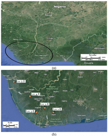
The study area is in Nigeria's Niger Delta, which has active soil known as the Niger flood zone. The annual rainfall of these areas is typically more than 2000 mm . As a result of the underlying terrain's flatness, drainage is impeded, resulting in poor lateralization of the very active (montmonillinitic) silty clay found there [46]. Furthermore, they swell and shrink upon contact with water, leading to the surface to be severely deformed, pavement cracking, and infrastructure failures [46]. In this regard, the active soil was enhanced using different nanomaterial-to-water ratios (1:50, 1:100, 1:150, 1:200, and 1:250), and the results were compared with untreated active from physical, chemical, and mechanical aspects. The results showed that including nanomaterials in active soil led to considerable change in the soil's physical, chemical, and mechanical characteristics by modifying its molecular structure. The soil's consistency and swelling potential were improved by decreasing the liquid limit, plasticity index, and shrinkage limit while increasing the plastic limit for different nanomaterial ratios.
Furthermore, the molecular-level hydrophobicity imparted by nanomaterial inclusion is highlighted in reducing water levels by offering a water-repellent zone on the stabilized surface. Moreover, the soil bearing and strength were considerably improved due to the pozzolanic reaction induced by adding nanomaterials. Additionally, the durability of the soil was significantly improved, reaching high values of 80% with a high nanomaterials ratio [46].
For model development, experimental data from five locations in the Niger Delta, namely Rivers-Atese (Loc 1-R), Rivers-Mbiama (Loc 2-R), Bayelsa-Opokuma (Loc 3-B), Bayelsa-Kiama (Loc 4-B), and Delta-Patani (Loc 5-D), as shown in Figure 1, are obtained from the literature [46]. A total of 60 datasets, 30 for crashing load and 30 for unconfined compressive strength prediction, are obtained. These data are represented in terms of plasticity index (PI), liquid limit (LL), natural moisture content (NMC), activity (A), clay content (C), and nanomaterial-to-water ratio (Mix per.), UCS and crushing load (q).
Figure 1. Case study area location (a) Nigeria's Niger Delta, (b) Data locations
2.2 MLP
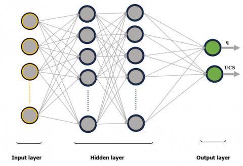
MLP is classified as an ANN type architecture and is regarded as the most dominant network in predictive and classification tasks due to its exceptional learning ability, enabling deeper connections to be made among data. MLP is composed of nodes known as perceptron arranged in layers [47]. Each layer in the MLP structure can be categorized as an input layer, where the features (input parameters) used for prediction are received; a hidden layer(s) (in this study are two), where the hidden features are being extracted and the output layer, where the outcomes (predictions) are determined. Furthermore, each layer consists of multiple interconnected neurons, with connections established through weight (ω), and bias (β). Figure 2(a) shows the structure of the MLP. Several factors influence the performance of the hidden layer, including the number of involved nodes and their activation functions [48]. Therefore, it is essential to configure the hidden layer properly to ensure good network performance. Eq. (1) determines neuron’s output (n) in the hidden layer.
$H_n=\varphi_1\left(\sum_{i=1}^I \omega_{n i} X_i+\beta_i\right)$ (1)
where, $\omega_{n i}$ and $\beta_i$ are the hidden layer's weights and biases and $\varphi_1(.)$ is the activation function. The network output $(\gamma)$ is illustrated in Eq. (2).
$\gamma=\varphi_2\left(\sum_{j=1}^J \omega_{k j} H_i+\beta_O\right)$ (2)
where, $\omega_{k j}$ and $\beta_0$ are weights and biases, respectively. $\varphi_2(.)$ is the output layer activation function.
2.3 GRNN
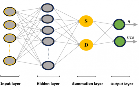
GRNN is a type of RBF proposed by Specht [49]. The GRNN computes the network’s output by employing the maximum probability approach, utilizing Parzen estimation based on nonparametric regression, and the available sample data serve as posterior conditions. The GRNN architecture comprises of four layers, namely the input, hidden, summation, and output layers, as illustrated in Figure 2(b). The GRNN's summation layer consists of two variations of neurons: the denominator unit, responsible for calculating the algebraic sum of each neuron in the hidden layer (as shown in Eq. (5)), and the molecular unit, which computes the weighted sum of each neuron in the hidden layer (as shown in Eq. (6)). The weights in this context represent the predicted training samples’ output values.
$S=\sum_{r=1}^R \omega_r e^{\left[-D\left(x, x_i\right)\right]}$ (3)
$D=\sum_{r=1}^R e^{\left[-D\left(x, x_i\right)\right]}$ (4)
The calculation of the predicted value of Y in the output layer is calculated by dividing the output of the molecular unit by denominator unit’s output as follows:
$Y(X)=\frac{S}{D}=\frac{\sum_{r=1}^R \omega_r \mathrm{e}^{\left[-D\left(x, x_i\right)\right]}}{D=\sum_{r=1}^R e^{\left[-D\left(x, x_i\right)\right]}}$ (5)
where $\omega_r$ and $R$ donate the weight and neurons number linked to the $r^{t h}$ neuron between the hidden layer and the summation layer. Moreover, the Gaussian function $\left(D\left(x, x_i\right)\right)$ can be mathematically expressed as follows:
$D\left(x, x_i\right)=\sum_{l=1}^{\mathrm{L}}\left(\frac{x_l-x_{i l}}{\theta_l}\right)^2$ (6)
where the input vector’s dimension is indicated in J. $x_l$ and $x_{i l}$ are the $l^{\text {th}}$ element of $x$ and $x_i$, respectively. Finally, $\theta_l$ represent the spread factor and to optimize the network, different spread factors are utilized several times until a minimum mean square error (MSE) value is reached or a predetermined threshold value.
2.4 RBF
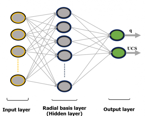
RBF is a feedforward neural network (FFNN) type that resembles MLP in terms of structure and is employed for a variety of tasks, including classification and regression. The main advantages of these networks are their ease of design, robustness to input noise, and speed and comprehensiveness of training, enabling them to map rather complicated nonlinear relationships. The RBF network architecture comprises three layers: input, hidden, and output, as depicted in Figure 2(c). The input parameters are received in the input layer, and the latter distributes them to the hidden layer. Moreover, radial basis functions are employed by the hidden layer to generate radial basis functions, while in the output layer, hidden neurons' outputs are linearly combined to generate the network outputs (predictions). The RBF output function can be mathematically expressed as follows:
$Y_i(x)=\sum_{j=1}^J \omega_{i j} \alpha\left(\left\|x-C_j\right\|\right)$ (7)
where, $x$ is the input vector, $Y_i$ is the network $\mathrm{i}^{\text {th}}$ output, $J$ is the hidden layer neurons number, $C_j$ refers to the $\mathrm{j}^{\text {th}}$ hidden neurons center, $\omega_{i j}$ is the weight, $\text {||. ||}$ refers to the Euclidian norm, and finally, $\alpha$ is the radial basis function, which, in this study, takes the form of the Gaussian function and can be mathematically expressed as follows:
$\alpha\left(\left\|X-C_i\right\|\right)=e^{\left(-\frac{\left\|X-C_j\right\|^2}{2 \delta_j^2}\right)}$ (8)
where, $\delta_j$ is the $\mathrm{j}^{\text {th}}$ hidden neuron width.
2.5 Model development and data preparation
The input parameters of this study are six presented in the PI, LL, NMC, activity (A), clay content (C), and nanomaterial-to-water ratio (Mix per.) to obtain two outputs presented in UCS and crushing load (q) using three machine learning models, namely MLP, RBF, and GRNN. The notion behind selecting these models because of their technical suitability and efficiency in related fields. The model's unique capacity to manage a rather complicated relationship, as well as computational efficiency and scalability, influenced the choosing process, making them suitable for capturing high dimensionality and intricate interrelationships among soil properties. The MLP model was chosen for its deep learning structure, enabling it to capture intricate patterns in high-dimensional data. The RBF model offers localized learning methodology and robustness to noise, enabling it to deal with spatially varying soil properties. Finally, the GRNN model offers nonparametric regression capabilities, enabling it to obtain smooth prediction, particularly with limited samples and undefined relationships. Moreover, these models have been proven in comparable fields [50-52].
The statistical description of all inputs and outputs is illustrated in Table 1. The collected data have been divided into three categories: training, which includes 70% of the data; validation, which includes 15% of the data; and testing, which includes the remaining 15% of the data.
The number of hidden layers has been chosen to be 1 layer for the GRNN and RBF and 2 layers for the MLP model, with 6 number of neurons in each layer for all models. Cross-validation is a highly recommended criterion for stopping the training of a network. For the current study, the stopping training process after 100 epochs and the lowest value of MSE will be considered. The activation function of all models used to be sigmoid. This study developed the suggested model using NeuroSolutions software version 7.1.1 on a Windows PC (core i7 12 gen CPU and 16 Gb RAM).
(a)
(b)
(c)
Figure 2. The structural configuration of (a) MLP, (b) RBF, and (c) GRNN
Table 1. The statistical characteristics of the input parameters
|
Statistics/Dataset |
NMC (%) |
LL (%) |
PI (%) |
C (%) |
A (%) |
q (kg) |
UCS (kN/m2) |
|
Maximum |
27.00 |
67.00 |
42.60 |
31.60 |
1.43 |
154.00 |
221.30 |
|
Minimum |
19.00 |
36.20 |
31.90 |
24.90 |
1.28 |
40.00 |
61.30 |
|
Average |
23.69 |
53.96 |
38.50 |
28.13 |
1.36 |
104.59 |
157.54 |
|
Standard deviation |
2.82 |
10.76 |
3.95 |
2.51 |
0.05 |
30.77 |
45.78 |
|
Skewness |
-0.63 |
-0.56 |
-0.66 |
0.10 |
-0.08 |
-0.7 |
-0.71 |
|
Confidence level (95%) |
1.07 |
4.09 |
1.5 |
0.96 |
0.02 |
11.71 |
17.41 |
2.6 Performance criteria
Assessing the performance of the proposed models is crucial in predicting the values of UCS and crushing load (q). In this regard, different statistical matrices have been implemented to examine the proposed models' prediction against the actual value obtained from the laboratory tests. These matrices are represented in normalized root mean square error (NRMSE), and normalized mean absolute error (NMAE) which asses the proposed models by measuring the size of the discrepancy between the actual and the predicted value. At the same time, another two matrices, namely correlation coefficient (CC) and coefficient of determination (R2) have been utilized for evaluating correlation and visualizing the closeness between the models’ prediction and the actual data [31, 53-55]. The performance matrices are obtained using Eqs. (9)-(12).
$N M A E=\frac{\frac{1}{n} \sum_{r=1}^n\left|\gamma_r-\breve{\gamma}_r\right|}{\bar{\gamma}}$ (9)
NRMSE $=\frac{\sqrt{\frac{1}{n} \sum_{r=1}^n\left(\gamma_r-\breve{\gamma}_r\right)^2}}{\bar{\gamma}}$ (10)
$R=\frac{\sum_{r=1}^n\left(\gamma_r-\bar{\gamma}\right)\left(\check{\gamma}_r-\check{\gamma}^m\right)}{\sqrt{\sum_{r=1}^n\left(\gamma_r-\bar{\gamma}\right)^2 \sum_{r=1}^n\left(\gamma_r-\check{\gamma}^m\right)^2}}$ (11)
$R^2=\frac{\frac{1}{n} \sum_{r=1}^n\left(\gamma_r-\bar{\gamma}\right)\left(\breve{\gamma}_r-\breve{\gamma}^m\right)}{\sqrt{\frac{1}{n} \sum_{r=1}^n\left(\gamma_r-\bar{\gamma}\right)^2} \sqrt{\frac{1}{n} \sum_{r=1}^n\left(\breve{\gamma}_r-\breve{\gamma}^m\right)}}$ (12)
where, $\gamma_r$ is the observed value, $\check{\gamma}_r$ is the predicted value, $\bar{\gamma}$ and $\check{\gamma}^m$ are the mean of the actual and predicted values, respectively.
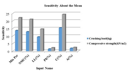
In this study, sensitivity analysis based on a modified Garson algorithm is performed to identify the input factor that most significantly impacts both the crushing load (q) and UCS. The method is more straightforward to implement by partitioning the output weights of neural network connections since it incorporates neural network tools within its framework [56]. The mathematical formulation of the algorithm is as follows:
$\theta=\frac{\sum_{j=1}^J\left|\omega_{i j} v_{j k}\right| / \sum_{r=1}^R\left|\omega_{r j}\right|}{\sum_{i=1}^I \sum_{j=1}^J\left(\left|\omega_{i j} v_{j k}\right| / \sum_{r=1}^R\left|\omega_{r j}\right|\right)}$ (13)
where, $\theta$ represents the impact of input’s parameter on the output, the wight $\omega_{i j}$ indicates the connection strength between the input and hidden neuron, and $v_{j k}$ signifies the weight connection strength between the hidden and the output neurons. Finally, $\omega_{r j}$ represents the weight connection between input’s neurons and the hidden layer. To ensure consistency and avoid the conflicting effects of positive and negative values, the connection weights are assigned their absolute values.
Figure 3. The impact of the input parameters on the crushing load and compressive strength
Figure 3 presents the sensitivity analysis results, illustrating the impact of each parameter on crushing load and compressive strength. It is worth noting that the sensitivity analysis highlights the importance of parameters, namely clay content, nanomaterial to water ratio, natural moisture content, and liquid limit, on the crushing load and compressive strength. In contrast, the importance of the other investigated parameters called plasticity index and activity of clay is less apparent. The clay content (C%) showed the most significant impact on both crashing load and unconfined compressive strength. This can be attributed to clay’s intrinsic properties, particularly its high surface area, enabling it to interact with nanomaterials through chemical bonding and pozzolanic reaction, improving the soil's strength, compressibility, and deformation. The second most influential factor is the nanomaterial-to-water ratio (Mix.per), highlighting its critical role in modifying soil properties. The pozzolanic reaction from adding nanomaterial to the investigated soil is the primary mechanism for improving soil’s properties by creating an additional bond between soil particles as well as reducing voids. This ratio governs the reaction efficiency as excess water may dilute the stabilization process, while insufficient water may hinder the reaction, highlighting the need to control this ratio precisely during practical applications. The third and fourth most influential factors are natural moisture content (NMC) and liquid limit (LL) due to their critical role in soil’s plasticity and its ability to retain water, which are considered critical factors for soil response to stabilization techniques. Higher moisture content can increase the potential of soil to swell and shrinkage, while liquid limit governs the soil stability under various water content. On the other hand, both plasticity index (PI) and activity (A) showed significantly low impact on both crashing load and unconfined compressive strength, which may be attributed to nanomaterial presence, where the latter can modify the chemical and structure of the soil.
This endeavor uses data from various locations in Nigeria's Niger Delta to develop and validate the proposed models taking into consideration two outcomes presented in crushing load (q) and UCS. The performance evaluation of the proposed models is evaluated through two distinct phases: training and testing. The performance during the training phase is depicted in Table 2 in terms of NRMSE, NMAE, and R. According to Table 2, the MLP model yields the best performance by delivering the highest prediction accuracy R=0.992 and 0.990 and lower prediction errors NMAE=0.036 and 0.035, NRMSE=0.043 for both q and UCS, respectively, providing a considerable generalization ability. Meanwhile, the RBF model provides the lowest performance for predicting q and UCS, providing high margins of errors and lower prediction accuracy.
Table 2. The performance matrices: Training phase
|
Model |
Output |
NRMSE |
NMAE |
R |
|
MLP |
q(Kg) |
0.043 |
0.036 |
0.992 |
|
UCS (kN/m2) |
0.043 |
0.035 |
0.990 |
|
|
RBF |
q(Kg) |
0.132 |
0.098 |
0.900 |
|
UCS (kN/m2) |
0.148 |
0.114 |
0.867 |
|
|
GRNN |
q(Kg) |
0.131 |
0.103 |
0.924 |
|
UCS (kN/m2) |
0.145 |
0.115 |
0.902 |
Table 3. The performance matrices: Testing phase
|
Model |
Output |
NRMSE |
NMAE |
R |
|
MLP |
q(Kg) |
0.139 |
0.122 |
0.962 |
|
UCS (kN/m2) |
0.118 |
0.099 |
0.978 |
|
|
RBF |
q(Kg) |
0.229 |
0.186 |
0.803 |
|
UCS (kN/m2) |
0.211 |
0.174 |
0.820 |
|
|
GRNN |
q(Kg) |
0.316 |
0.280 |
0.817 |
|
UCS (kN/m2) |
0.300 |
0.266 |
0.837 |
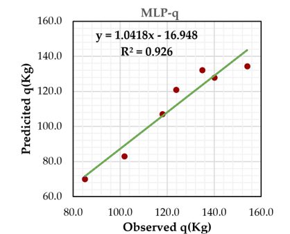
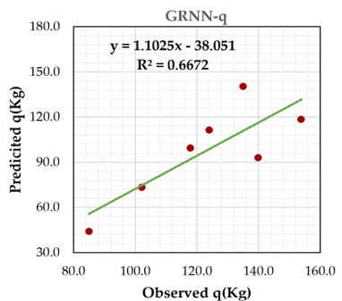
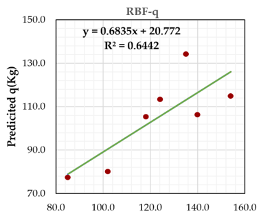
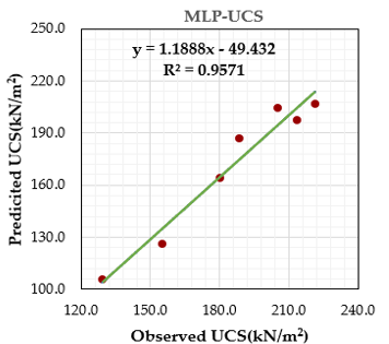
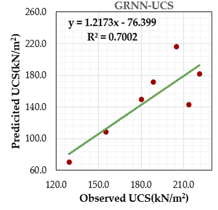
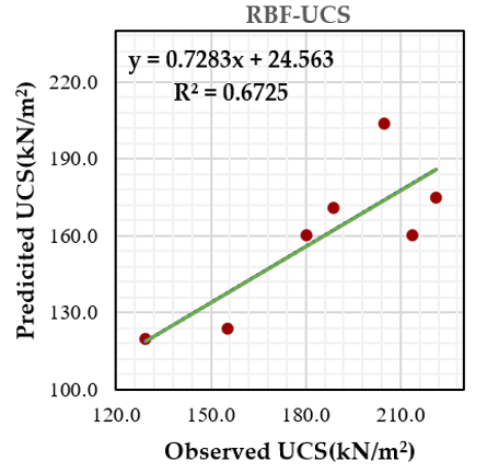
On the other hand, the testing phase results for the proposed models are displayed in Table 3, highlighting their performance. Furthermore, the accuracy of the proposed model has also been measured by employing the coefficient of determination (R2) as presented in Figures 4 and 5, which is a statistical metric that quantifies the relationship between the predicted and actual values, indicating the level of correlation between them. The ideal correlation is achieved when R2=1, and all data points align perfectly on a line that passes through the origin, resulting in a 45° angle. According to Table 3, the MLP model outperforms both RBF and GRRN models in predicting q and UCS, providing significantly high R-value and lower NMAE and NRMSE values. Furthermore, Figures 4(a) and 5(a) show the scatter plot between the actual and predicted data samples, showing that the MLP model exhibits the highest R2 value for both q and UCS with a value of 0.926 and 0.957, respectively. Additionally, the data samples exhibit proximity to the line, indicating the effectiveness of the MLP model in accurately predicting the crashing load and compressive strength. Moreover, the MLP can predict UCS more efficiently with R2, R, NMAE, and NRMSE values of 0.957, 0.978, 0.099, and 0.118, respectively. On the other hand, the GRNN and RBF models showed an inferior performance in predicting q and UCS, providing higher prediction errors in terms of NMAE and NRMSE and lower prediction performance in terms of R. Figures 4(b), 5(b), 4(c), and 5(c) show the scatter plot of both models in predicting crushing load and compressive strength. According to Figures 4(b) and 5(b), the data samples for GRRN are scattered away around the line, with R2 values 0.667 and 0.700 in terms of q and UCS, respectively, which is the same case for the RBF model (see Figures 4(c) and 5(c)) with R2 values 0.644 and 0.672 terms of q and UCS, respectively. Additionally, the performance of both models in predicting compressive strength is slightly better than that of the crushing load.
(a)
(b)
(c)
Figure 4. The scatter plot between actual and predicted values for crushing load (a) MLP, (b) GRNN, and (c) RBF
(a)
(b)
(c)
Figure 5. The scatter plot between actual and predicted values for unconfined compressive strength (a) MLP, (b) GRNN, and (c) RBF
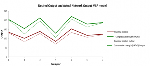
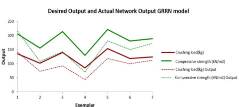
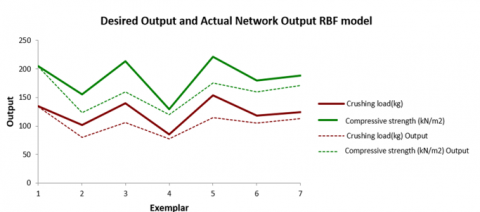
Figure 6 depicts the actual value against the predicted value, which, in this case, q and UCS, for each model. Figure 5 demonstrates the superiority of the MLP model for simulating the peak values of compressive strength and crushing load, which is the same case for the lower values (see Figure 6(a)). On the contrary, the GRRN and RBF models are unable to simulate the actual values of the compressive strength and crushing load (see Figures 6(b) and 6(c)).
The superiority of the MLP model is attributed to its advanced deep learning structure, allowing it to capture complex patterns and nonlinear relationships within the dataset. On the other hand, RBF and GRNN have simple architectures and predefined kernel or regression functions. Meanwhile, the MLP model’s parameters are dynamically adjusted during training, allowing it to capture intricate interactions among the six soil parameters. Moreover, the MLP utilizes a nonlinear activation function to improve the model's flexibility, enabling it to process high-dimensional data that the shallow structure of the other models might miss. Additionally, the backpropagation technique allows the MLP model to minimize the prediction error iteratively and optimize the weights, ensuring the best performance in cases of noise or variability in the data.
(a)
(b)
(c)
Figure 6. Comparison between actual and predicted for both the crushing load and compressive strength values (a) MLP, (b) GRNN, and (c) RBF
This study explores the potential of ML models in predicting the crushing load and compressive strength of nanomaterials stabilized active soil. Accordingly, three AI models have been implemented, namely, MLP, RBF, and GRNN. The proposed models’ performance is assessed through the training and testing phases, using different statistical matrices and graphical appraisals. The finding showed that the MLP model provides authentic predictions and generalization abilities with R^2 values of 0.926 and 0.957 for both crashing load and compressive strength, respectively. Furthermore, the MLP model exhibited better performance in predicting compressive strength compared to crushing load. Meanwhile, the RBF and GRNN, despite having a considerable performance in the training phase, showed significantly poor performance in the testing phase. The MLP model's superiority denotes its deep learning architecture, which is ideal for complex, non-linear data patterns, making the model typical in soil properties. Additionally, MLP structure allows for effective learning of high-dimensional data and intricate interactions. On the contrary, the RBF and GRNN models, while initially performing well in training, likely due to overfitting issues, influencing their generalization to new data. The robustness of the MLP model is enhanced by optimal tuning of the parameters, mimicking the specific characteristics of the soil property dataset, leading to more accurate predictions. From the practical perspective, leveraging the MLP model paves the way for engineers to predict soil’s critical parameters, which in turn reduces the reliance on resource-intensive and time-consuming experiments, particularly in soil stabilization practices.
Finally, sensitivity analyses are established to investigate the impact of the input parameters on the crashing load and compressive strength, showing that the clay content (C) has the most impact on both outputs, followed by the nanomaterial-to-water ratio (Mix per.), NMC, and LL.
In light of these findings, this study suggests investigating other advanced neural network types, such as CNN and recurrent neural networks (RNNs), which may increase prediction accuracy and generalization ability. Furthermore, incorporating other soil parameters, such as permeability and shear strength, to obtain a more comprehensive understanding of soil behaviour during the stabilization process. Moreover, utilizing hybrid models incorporates vanilla models with bio-inspired algorithms such as genetic algorithm (GA) or particle swarm optimization (PSO), which refine the model’s output and optimize input parameters.
|
q |
Crashing load Kg |
|
UCS |
Unconfined compressive strength kN/m2 |
|
LL |
Liquid limit (%) |
|
PL |
Plastic limit (%) |
|
NMC |
Normal moisture content (%) |
|
A |
Activity (dimensionless) |
|
C |
Clay content (%) |
|
Mix per. |
Nanomaterial-to-water ratio (dimensionless) |
|
$\varphi$ |
Activation function for MLP (dimensionless) |
|
$\theta$ |
Spread factor for GRNN (dimensionless) |
|
$\alpha$ |
Radial basis function for RBF (dimensionless) |
|
$\delta$ |
Jth hidden layer width for RBF (dimensionless) |
|
σ |
Gaussian function parameter (dimensionless) |
|
$\omega$ |
Weight (dimensionless, refers to neural network weights in MLP/RBF/GRNN models) |
|
Subscripts |
|
|
AI |
Artificial intelligence |
|
MLP |
Multilayer perceptron |
|
GRNN |
Generalize regression neural network |
|
RBF |
Radial basis function neural network |
|
NRMSE |
Normalized root mean square error (dimensionless) |
|
NMAE |
Normalized mean absolute error (dimensionless) |
|
R |
Correlation coefficient (dimensionless) |
|
R2 |
Coefficient of determination (dimensionless) |
[1] Abiodun, A.A., Nalbantoglu, Z. (2015). Lime pile techniques for the improvement of clay soils. Canadian Geotechnical Journal, 52(6): 760-768. https://doi.org/10.1139/cgj-2014-0073
[2] Chen, F.H. (2012). Foundations on Expansive Soils. Elsevier.
[3] Karumanchi, M., Avula, G., Pangi, R., Sirigiri, S. (2020). Improvement of consistency limits, specific gravities, and permeability characteristics of soft soil with nanomaterial: Nanoclay. Materials Today: Proceedings, 33: 232-238. https://doi.org/10.1016/j.matpr.2020.03.832
[4] Liu, G., Zhang, C., Zhao, M., Guo, W., Luo, Q. (2020). Comparison of nanomaterials with other unconventional materials used as additives for soil improvement in the context of sustainable development: A review. Nanomaterials, 11(1): 15. https://doi.org/10.3390/nano11010015
[5] Mir, B.A., Reddy, S.H. (2021). Enhancement in shear strength characteristics of soft soil by using nanomaterials. In Sustainable Environmental Infrastructure, pp. 421-435. https://doi.org/10.1007/978-3-030-51354-2_39
[6] Kulanthaivel, P., Soundara, B., Velmurugan, S., Naveenraj, V. (2021). Experimental investigation on stabilization of clay soil using nano-materials and white cement. Materials Today: Proceedings, 45: 507-511. https://doi.org/10.1016/j.matpr.2020.02.107
[7] Karumanchi, M., Nerella, R. (2022). Influence of extracted nanosilica on geotechnical properties of soft-clay soil subjected to freeze-thaw cycles. Journal of Building Pathology and Rehabilitation, 7(1): 43. https://doi.org/10.1007/s41024-022-00179-w
[8] Li, B., Luo, F., Ai, X., Li, X., Li, L. (2022). Mechanical properties of unbound granular materials reinforced with nanosilica. Case Studies in Construction Materials, 17: e01574. https://doi.org/10.1016/j.cscm.2022.e01574
[9] Choobbasti, A.J., Samakoosh, M.A., Kutanaei, S.S. (2019). Mechanical properties of soil stabilized with nano calcium carbonate and reinforced with carpet waste fibers. Construction and Building Materials, 211: 1094-1104. https://doi.org/10.1016/j.conbuildmat.2019.03.306
[10] Jalal, F.E., Xu, Y., Jamhiri, B., Memon, S.A. (2020). On the recent trends in expansive soil stabilization using calcium-based stabilizer materials (CSMs): A comprehensive review. Advances in Materials Science and Engineering, 2020(1): 1510969. https://doi.org/10.1155/2020/1510969
[11] Vaganova, N.A., Filimonov, M.Y. (2019). Simulation of cooling devices and effect for thermal stabilization of soil in a cryolithozone with anthropogenic impact. In International Conference on Finite Difference Methods, pp. 580-587. https://doi.org/10.1007/978-3-030-11539-5_68
[12] Ghavami, S., Naseri, H., Jahanbakhsh, H., Nejad, F.M. (2021). The impacts of nano-SiO2 and silica fume on cement kiln dust treated soil as a sustainable cement-free stabilizer. Construction and Building Materials, 285: 122918. https://doi.org/10.1016/j.conbuildmat.2021.122918
[13] Maichin, P., Jitsangiam, P., Nongnuang, T., Boonserm, K., Nusit, K., Pra-Ai, S., Binaree, T., Aryupong, C. (2021). Stabilized high clay content lateritic soil using cement-FGD gypsum mixtures for road subbase applications. Materials, 14(8): 1858. https://doi.org/10.3390/ma14081858
[14] Wang, L., Cho, D.W., Tsang, D.C.W., Cao, X., Hou, D., Shen, Z., Alessi, D.S., Ok, Y.S., Poon, C.S. (2019). Green remediation of As and Pb contaminated soil using cement-free clay-based stabilization/solidification. Environmental International, 126: 336-345. https://doi.org/10.1016/j.envint.2019.02.057
[15] Liu, Y., Chang, C.W., Namdar, A., She, Y., Lin, C.H., Yuan, X., Yang, Q. (2019). Stabilization of expansive soil using cementing material from rice husk ash and calcium carbide residue. Construction and Building Materials, 221: 1-11. https://doi.org/10.1016/j.conbuildmat.2019.05.157
[16] Jiang, N., Wang, C., Wang, Z., Li, B., Liu, Y. (2021). Strength characteristics and microstructure of cement stabilized soft soil admixed with silica fume. Materials, 14(8): 1929. https://doi.org/10.3390/ma14081929
[17] Zeng, L.L., Bian, X., Zhao, L., Wang, Y.J., Hong, Z.S. (2021). Effect of phosphogypsum on physiochemical and mechanical behaviour of cement stabilized dredged soil from Fuzhou, China. Geomechanics and Energy Environment, 25: 100195. https://doi.org/10.1016/j.gete.2020.100195
[18] Cuisinier, O., Le Borgne, T., Deneele, D., Masrouri, F. (2011). Quantification of the effects of nitrates, phosphates and chlorides on soil stabilization with lime and cement. Engineering Geology, 117(3-4): 229-235. https://doi.org/10.1016/j.enggeo.2010.11.002
[19] Etim, R.K., Eberemu, A.O., Osinubi, K.J. (2017). Stabilization of black cotton soil with lime and iron ore tailings admixture. Transportation Geotechnics, 10: 85-95. https://doi.org/10.1016/j.trgeo.2017.01.002
[20] Tremblay, H., Duchesne, J., Locat, J., Leroueil, S. (2002). Influence of the nature of organic compounds on fine soil stabilization with cement. Canadian Geotechnical Journal, 39(3): 535-546. https://doi.org/10.1139/t02-002
[21] Rosales, J., Agrela, F., Marcobal, J.R., Diaz-López, J.L., Cuenca-Moyano, G.M., Caballero, Á., Cabrera, M. (2020). Use of nanomaterials in the stabilization of expansive soils into a road real-scale application. Materials, 13(14): 3058. https://doi.org/10.3390/ma13143058
[22] Abdullah, H.H., Shahin, M.A., Walske, M.L. (2020). Review of fly-ash-based geopolymers for soil stabilisation with special reference to clay. Geosciences, 10(7): 249. https://doi.org/10.3390/geosciences10070249
[23] Mashifana, T.P., Okonta, F.N., Ntuli, F. (2018). Geotechnical properties and microstructure of lime-fly ash-phosphogypsum-stabilized soil. Advances in Civil Engineering, 2018(1): 3640868. https://doi.org/10.1155/2018/3640868
[24] Pliaka, M., Gaidajis, G. (2022). Potential uses of phosphogypsum: A review. Journal of Environmental Science and Health, Part A, 57(9): 746-763. https://doi.org/10.1080/10934529.2022.2105632
[25] Galvín, A.P., López-Uceda, A., Cabrera, M., Rosales, J., Ayuso, J. (2021). Stabilization of expansive soils with biomass bottom ashes for an eco-efficient construction. Environmental Science and Pollution Research, 28: 24441-24454. https://doi.org/10.1007/s11356-020-08768-3
[26] Iyaruk, A., Promputthangkoon, P., Lukjan, A. (2022). Evaluating the performance of lateritic soil stabilized with cement and biomass bottom ash for use as pavement materials. Infrastructures, 7(5): 66. https://doi.org/10.3390/infrastructures7050066
[27] Mozejko, C.A., Francisca, F.M. (2020). Enhanced mechanical behavior of compacted clayey silts stabilized by reusing steel slag. Construction and Building Materials, 239: 117901. https://doi.org/10.1016/j.conbuildmat.2019.117901
[28] Yildirim, I.Z., Prezzi, M. (2022). Subgrade stabilisation mixtures with EAF steel slag: An experimental study followed by field implementation. International Journal of Pavement Engineering, 23(6): 1754-1767. https://doi.org/10.1080/10298436.2020.1823389
[29] Tomar, A., Sharma, T., Singh, S. (2020). Strength properties and durability of clay soil treated with a mixture of nano silica and polypropylene fiber. Materials Today: Proceedings, 26: 3449-3457. https://doi.org/10.1016/j.matpr.2019.12.239
[30] Arora, A., Singh, B., Kaur, P. (2019). Performance of nanoparticles in stabilization of soil: A comprehensive review. Materials Today: Proceedings, 17: 124-130. https://doi.org/10.1016/j.matpr.2019.06.409
[31] Hameed, M.M., Khaleel, F., Khaleel, D. (2021). Employing a robust data-driven model to assess the environmental damages caused by installing grouted columns. In 2021 Third International Sustainability and Resilience Conference: Climate Change, Sakheer, Bahrain, pp. 305-309. https://doi.org/10.1109/IEEECONF53624.2021.9668027
[32] Sundararajan, N., Habeebsheriff, H.S., Dhanabalan, K., Cong, V.H., Wong, L.S., Rajamani, R., Dhar, B.K. (2024). Mitigating global challenges: Harnessing green synthesized nanomaterials for sustainable crop production systems. Global Challenges, 8(1): 2300187. https://doi.org/10.1002/gch2.202300187
[33] Teizer, J., Venugopal, M., Teizer, W., Felkl, J. (2012). Nanotechnology and its impact on construction: Bridging the gap between researchers and industry professionals. Journal of Construction Engineering and Management, 138(5): 594-604. https://doi.org/10.1061/(ASCE)CO.1943-7862.0000467
[34] Kong, R., Zhang, F., Wang, G., Peng, J. (2018). Stabilization of loess using nano-SiO2. Materials, 11(6): 1014. https://doi.org/10.3390/ma11061014
[35] Liu, C., Zhang, Q., Zhao, C., Deng, L., Fang, Q. (2023). Assessment of strength development of soil stabilized with cement and nano-SiO2. Construction and Building Materials, 409: 133889. https://doi.org/10.1016/j.conbuildmat.2023.133889
[36] Khodabandeh, M.A., Nagy, G., Török, Á. (2023). Stabilization of collapsible soils with nanomaterials, fibers, polymers, industrial waste, and microbes: Current trends. Construction and Building Materials, 368: 130463. https://doi.org/10.1016/j.conbuildmat.2023.130463
[37] Onyelowe, K.C., Ebid, A.M., Onyia, M.E., Nwobia, L.I. (2021). Predicting nanocomposite binder improved unsaturated soil UCS using genetic programming. Nanotechnology for Environmental Engineering, 6: 39. https://doi.org/10.1007/s41204-021-00134-z
[38] Rajaei, P., Baladi, G.Y. (2015). Frost depth: General prediction model. Transportation Research Record, 2510(1): 74-80. https://doi.org/10.3141/2510-09
[39] Gandomi, A.H., Alavi, A.H. (2011). Multi-stage genetic programming: A new strategy to nonlinear system modeling. Information Sciences, 181(23): 5227-5239. https://doi.org/10.1016/j.ins.2011.07.026
[40] Soleimani, S., Rajaei, S., Jiao, P., Sabz, A., Soheilinia, S. (2018). New prediction models for unconfined compressive strength of geopolymer stabilized soil using multi-gen genetic programming. Measurement, 113: 99-107. https://doi.org/10.1016/j.measurement.2017.08.043
[41] Tabarsa, A., Latifi, N., Osouli, A., Bagheri, Y. (2021). Unconfined compressive strength prediction of soils stabilized using artificial neural networks and support vector machines. Frontiers of Structural and Civil Engineering, 15(2): 520-536. https://doi.org/10.1007/s11709-021-0689-9
[42] Onyelowe, K.C., Ebid, A.M., Nwobia, L., Dao-Phuc, L. (2021). Prediction and performance analysis of compression index of multiple-binder-treated soil by genetic programming approach. Nanotechnology for Environmental Engineering, 6(2): 28. https://doi.org/10.1007/s41204-021-00123-2
[43] Nguyen, T., Ly, K.D., Nguyen-Thoi, T., Nguyen, B.P., Doan, N.P. (2022). Prediction of axial load bearing capacity of PHC nodular pile using Bayesian regularization artificial neural network. Soils and Foundations, 62(5): 101203. https://doi.org/10.1016/j.sandf.2022.101203
[44] Qian, Z.G., Li, A.J., Chen, W.C., Lyamin, A.V., Jiang, J.C. (2019). An artificial neural network approach to inhomogeneous soil slope stability predictions based on limit analysis methods. Soils and Foundations, 59(2): 556-569. https://doi.org/10.1016/j.sandf.2018.10.008
[45] Chen, Q., Hu, G., Wu, J. (2024). Prediction of the unconfined compressive strength of a one-part geopolymer-stabilized soil using deep learning methods with combined real and synthetic data. Buildings, 14(9): 2894. https://doi.org/10.3390/buildings14092894
[46] Ugwu, O.O., Ogboin, A.S., Nwoji, C.U. (2018). Characterization of engineering properties of active soils stabilized with nanomaterial for sustainable infrastructure delivery. Frontiers in Built Environment, 4: 65. https://doi.org/10.3389/fbuil.2018.00065
[47] Kuo, P.H., Huang, C.J. (2018). A high precision artificial neural networks model for short-term energy load forecasting. Energies, 11(1): 213. https://doi.org/10.3390/en11010213
[48] Suliman, A., Zhang, Y. (2015). A review on back-propagation neural networks in the application of remote sensing image classification. Journal of Earth Science and Engineering, 5(1): 52-65. https://doi.org/10.17265/2159-581X/2015.01.004
[49] Specht, D.F. (1991). A general regression neural network. IEEE Transactions on Neural Networks, 2(6): 568-576. https://doi.org/10.1109/72.97934
[50] Moayedi, H., Moatamediyan, A., Nguyen, H., Bui, X.N., Bui, D.T., Rashid, A.S.A. (2020). Prediction of ultimate bearing capacity through various novel evolutionary and neural network models. Engineering Computations, 36(2): 671-687. https://doi.org/10.1007/s00366-019-00723-2
[51] Verma, G., Kumar, B. (2022). Multi-layer perceptron (MLP) neural network for predicting the modified compaction parameters of coarse-grained and fine-grained soils. Innovative Infrastructure Solutions, 7(1): 78. https://doi.org/10.1007/s41062-021-00679-7
[52] Kumar, A., Sinha, S., Saurav, S., Chauhan, V.B. (2023). Prediction of unconfined compressive strength of cement-fly ash stabilized soil using support vector machines. Asian Journal of Civil Engineering, 25(2): 1149-1161. https://doi.org/10.1007/s42107-023-00833-9
[53] El-Shafie, A., Noureldin, A., Taha, M., Hussain, A., Mukhlisin, M. (2012). Dynamic versus static neural network model for rainfall forecasting at Klang River Basin, Malaysia. Hydrology and Earth System Sciences, 16(4): 1151-1169. https://doi.org/10.5194/hess-16-1151-2012
[54] Shariat, M., Shariati, M., Madadi, A., Wakil, K. (2018). Computational Lagrangian multiplier method by using for optimization and sensitivity analysis of rectangular reinforced concrete beams. Steel and Composite Structures, 29(2): 243-256. https://doi.org/10.12989/scs.2018.29.2.243
[55] Khaleel, F., Hameed, M.M., Khaleel, D., AlOmar, M.K. (2022). Applying an efficient AI approach for the prediction of bearing capacity of shallow foundations. In International Conference on Emerging Technology Trends in Internet of Things and Computing, Springer, pp. 310-323. https://doi.org/10.1007/978-3-030-97255-4_23
[56] Kamel, A.H., Afan, H.A., Sherif, M., Ahmed, A.N., El-Shafie, A. (2021). RBFNN versus GRNN modeling approach for sub-surface evaporation rate prediction in arid regions. Sustainable Computing: Informatics and Systems, 30: 100514. https://doi.org/10.1016/j.suscom.2021.100514