Manh-Tung Ngo![]() | Yen-Vu Thi
| Yen-Vu Thi![]() | Van-Cuong Pham
| Van-Cuong Pham![]() | Dinh-Chung Dang
| Dinh-Chung Dang![]() | Hong-Quang Nguyen*
| Hong-Quang Nguyen*![]()
© 2025 The authors. This article is published by IIETA and is licensed under the CC BY 4.0 license (http://creativecommons.org/licenses/by/4.0/).
OPEN ACCESS
The problem of balancing a two-wheeled bicycle robot is a problem that attracts many researchers. The bicycle robot model is usually a nonlinear model. However, to simplify the control design process, the bicycle robot model is often linearized into a linear model. The design of a bicycle robot balance controller using a robust control algorithm, based on the linear model of the bicycle robot, often results in a high-order controller (original controller). A high-order controller will make the control program code complex and may reduce the quality of the control system. To make the controller simpler, the paper applied the model order reduction algorithm (ORA) to determine the low-order robust controllers. Through comparison and analysis of the low-order controllers, the paper selected the second-order controller as the most suitable controller to replace the original controller. At the same time, the paper also evaluates the efficiency of the control system when using a second-order controller in the case of a bicycle robot model that is a nonlinear model and a linear model, thereby determining the application limits of the second-order controller.
bicycle robot, robust control, nonlinear model, model order reduction, balanced truncation method
The most difficult and fascinating issue in bicycle robot research is maintaining the robot's ability to balance. Bicycle robot is one of the types of robots that many researchers are interested in this field. There are many methods to solve the problem of balancing bicycle robots, such as the flywheel balancing method [1-13], the centrifugal force balancing method [14, 15], and the center of gravity shifting balancing method [16]. In this paper, we focus on the flywheel balancing bicycle robot model based on the inverted pendulum principle, with the main characteristics that the flywheel usually rotates at low speed and consumes little energy, and the robot has stable balance when standing still and moving.
Because the operating condition of a bicycle robot is affected by several uncertain factors suchlike usage load, outside force effect, etc., in most studies on bicycle robot modeling, the bicycle robot model is considered a tentative model. There are many control algorithms proposed to design the bicycle robot balance controller, such as the Proportional Integral Derivative (PID) algorithm [1, 7, 8], Proportional Derivative (PD) algorithm [10], Linear–Quadratic–Gaussian (LQG) [4] and Model Predictive Control (MPC) control [2, 3, 9]. However, suppose the robot model is considered as an uncertain model. In that case, the sustainable and optimally stable control algorithm is regarded as the most suitable for the robot balance controller design problem [5, 12, 13].
Controllers designed based on robust control algorithms are often high-order. High-order controllers often lead to complex control program codes that increase the processing time of the controller, which in turn increases the response time of the control system. Slow response time of the control system can cause the bicycle robot to oscillate more strongly or the robot to lose stability. Therefore, along with the problem of designing a robust controller, there is often the problem of determining a low-order robust controller that can replace the high-order controller to simultaneously satisfy the two requirements of robust control and simple control. The first way is to simplify the controller right during the design of the robust controller, in this way, after the design process, the authors will get the low-order stable controller [5]. The second way is to apply the order reduction algorithm (ORA) to simplify the controller obtained from the controller design process based on the robust control algorithm [12-14]. According to many studies, the first way has higher computational complexity than the second way [12-14]. At the same time, in the first way, when the order of the low-order controller is chosen unreasonably, it may make the problem of finding the controller parameters ineffective. With the second way, the low-order controller will always be defined in all cases. However, to find a suitable low-order controller, it is necessary to compare and evaluate the low-order controllers obtained by the order reduction method. Previous studies [5, 6, 12-14] often only compare the low-order controllers obtained by a specific order reduction algorithm. But in fact, there are many different order reduction algorithms, so when applying these algorithms to the order reduction problem, high-order controllers will obtain low-order controllers. Therefore, it is necessary to compare and evaluate the low-order controllers obtained from different order reduction algorithms to find the most suitable low-order controller. At the same time, in previous studies [5, 6, 12-14], the influence of linearization of the bicycle robot model on the stability of the control system when using a strong low-order controller has not been studied and evaluated. Therefore, in this study, the author will focus on the problem of determining the most suitable low-order controller to replace the high-order controller and at the same time consider and evaluate the effect of linearizing the bicycle robot model on the stability of the control system when using the low-order controller.
The paper is organized as follows: The introduction is presented in Section 1; Section 2 introduces the kinematic model of the bicycle robot; the design process of a robust controller for the robotic bicycle balance system is presented in Section 3; Section 4 presents the order reduction results of the high-order robust controller; Section 5 presents the conclusion.
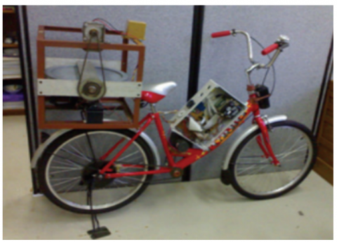
A bicycle robot was based on a typical bicycle to test the control algorithms [5, 6]. A flywheel system is arranged on the robot to help it maintain an upright stand. When the flywheel system (which is rotating around the Y-axis at a constant speed) is driven around the Z-axis with an offset angle j, the flywheel system generates a torque that opposes the gravity torque. When the robot deviates from the vertical position with an inclined angle q, a moment of gravity will cause the robot to fall. A DC motor drives the flywheel to rotate around the Z axis. The task is to design a controller to change the voltage supplied to the motor, thereby helping the robot maintain a state of balance, i.e., the robot tilt angle q always approaches zero. Figure 1 describes the details of the robot as follows:
(a) Bicycle robot model
(b) Diagram of reference coordinates of bicycle robot
Figure 1. Detailed model and projection model of bicycle robot [5, 6]
The dimensions of the robot are described in references [5, 6], where the robot uses a DC motor to rotate the flywheel.
Based on the description of the kinematics of the bicycle robot using the Lagrange equation, the authors in references [5, 6] have built a mathematical model of the robot, with the following results:
$\begin{aligned} & \ddot{\theta}\left[m_b h_b^2+m_f h_f^2+I_b+I_p \sin ^2 \varphi+I_r \cos ^2 \varphi\right] +2 \sin \varphi \cos \varphi\left(I_p-I_r\right) \dot{\theta} \dot{\varphi} -g\left(m_b h_b+m_f h_f\right) \sin \theta =I_p \omega \dot{\varphi} \cos \varphi\end{aligned}$ (1)
$\begin{aligned} & \ddot{\varphi} I_r-\dot{\theta}^2\left(I_p-I_r\right) \sin \varphi \cos \varphi =5 K_m\left(\frac{U-L d i / d t-K_e \dot{\varphi}}{R}\right)-I_p \omega \dot{\theta} \cos \varphi-B_m \dot{\varphi}\end{aligned}$ (2)
where, i is the current and U is the voltage of the DC motor.
From Eqs. (1) and (2), it can be seen that the dynamic model of the robot is a nonlinear model. Table 1 shows the technical specifications of the robot model.
Table 1. The technical specifications of the robot model
|
Parameter |
Value |
Unit |
|
$I_p$ |
0.215926 |
Kg.m2 |
|
$I_r$ |
0.215926 |
Kg.m2 |
|
$I_b$ |
27.584 |
Kg.m2 |
|
$h_b$ |
0.8 |
m |
|
$h_f$ |
0.86 |
m |
|
$m_b$ |
43.1 |
Kg |
|
$m_f$ |
8.1 |
Kg |
|
$K_e$ |
0.215926 |
V.s/Rad |
|
$K_m$ |
0.215926 |
N.m/A |
|
$B_m$ |
0.000253 |
Kg.2/s |
|
$R$ |
0.41 |
$\Omega$ |
|
$L$ |
0.0006 |
H |
|
$g$ |
9.81 |
m/s2 |
The robot's equilibrium position is the position with the tilt angle $\theta$=0. The task of the balance control system is to always maintain the robot's tilt angle at the robot's equilibrium position. In fact, to ensure that the balance control system works well, the robot's tilt angle is only allowed to fluctuate around the equilibrium position with a small value ($\theta \leq 1.5^{\circ}$). If the robot's tilt angle is too large, the balance control system cannot maintain the robot's equilibrium (because the moment of the flywheel system is not enough to balance the moment of the robot's gravity). Therefore, to linearize Eqs. (1) and (2), we perform linearization around the robot's equilibrium position ($\theta=\varphi \leq 1.5^{\circ}, \sin \theta=\sin \psi \approx 0$), the results obtained are as follows [5, 6]:
$\begin{aligned} & \left(m_b h_b^2+m_f h_f^2+I_b+I_r\right) \ddot{\theta} -g\left(m_b h_b+m_f h_f\right) \theta-I_p \omega \dot{\varphi}=0\end{aligned}$ (3)
$\begin{aligned} & I_r \ddot{\varphi}+I_p \omega \dot{\theta}+B_m \dot{\varphi} -5 K_m\left[\frac{U-L d i / d t-K_e \dot{\varphi}}{R}\right]=0\end{aligned}$ (4)
Let $x=\left[\begin{array}{c}\theta=x_1 \\ \dot{\theta}=x \\ \dot{\varphi}=x_3 \\ \dot{l}=x_4\end{array}\right]$ be the state variable, $y=\theta, u=U$.
The authors have the following equations of state describing the bicycle robot:
$\begin{aligned} \dot{x} & =\mathbf{A} x+\mathbf{B} u \\ y & =\mathbf{C} x+\mathbf{D} u\end{aligned}$ (5)
The matrices of the state Eq. (5) have the following form [5, 6]:
$\begin{gathered}\mathbf{A}=\left[\begin{array}{cccc}0 & 1 & 0 & 0 \\ \frac{g\binom{m_b h_b}{+m_f h_f}}{m_b h_b^2+m_f h_f^2} & 0 & \frac{I_p \omega}{m_b h_b^2+m_f h_f^2} & 0 \\ +I_b+I_r & & +I_b+I_r & \\ 0 & -\frac{I_p \omega}{I_r} & -\frac{B_m}{I_r} & \frac{5 K_m}{I_r} \\ 0 & 0 & -\frac{K_e}{L} & -\frac{R}{L}\end{array}\right], \\ \mathbf{B}=\left[\begin{array}{c}0 \\ 0 \\ 0 \\ 1 / L\end{array}\right], \mathbf{C}=\left[\begin{array}{llll}1 & 0 & 0 & 0\end{array}\right], \mathbf{D}=[0]\end{gathered}$
Using the specifications of Table 1 to determine the parameters of the matrices of the state Eq. (5), the authors get the following results [5, 6]:
$\begin{gathered}\mathbf{A}=\left[\begin{array}{cccc}0 & 1 & 0 & 0 \\ 6.6358 & 0 & 0.5536 & 0 \\ 0 & -302.016 & -0.0023 & 5.2981 \\ 0 & 0 & -197.33 & -683.33\end{array}\right], \\ \mathbf{B}=\left[\begin{array}{c}0 \\ 0 \\ 0 \\ 1666.7\end{array}\right], \mathbf{C}=\left[\begin{array}{llll}1 & 0 & 0 & 0\end{array}\right], D=[0]\end{gathered}$
Converting the state model of the robot to the transfer function model, the authors have the result [5, 6]:
$\mathbf{S}(s)=\frac{\boldsymbol{\theta}(s)}{\mathbf{U}(s)}=\frac{4888}{s^4+683.3 s^3+128 s^2+109700 s-6949}$ (6)
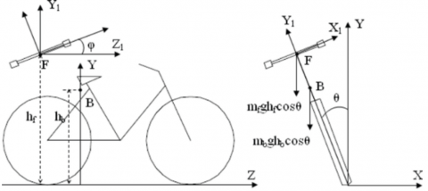
A control system for the bicycle robot based on the robust control structure diagram is designed as shown in Figure 2.
Figure 2. Block diagram describing the control system for the bicycle robot
Design a robust controller according to references [6, 17], specifically as follows:
Step 1: The first S object is formatted 2 by W2 and W2 to achieve the required open-loop form. (W1, W2 are the pre-compensator and post-compensator respectively) $S_s=\mathbf{W}_2 \mathbf{S W}_1$.
With $\boldsymbol{W}_{\mathbf{1}}(s)=\boldsymbol{K} \frac{s+\alpha_1}{s+\beta_1}$ and $\boldsymbol{W}_2(s)=\boldsymbol{K} \frac{s+\alpha_1}{s+\beta_1}$.
After selecting W1 and W2, the $\gamma_{\text {opt }}$ value is calculated using to the following formula (The details of the calculation process $\gamma_{\text {opt }}$ are shown in the document [17]):
$\gamma_{\text {opt }}=\left[1+\lambda_{\max }(\mathbf{Z X})\right]^{1 / 2}$ (7)
where, Z and X are determined from the following Riccati equation:
$\begin{gathered}\left(\mathbf{A}-\mathbf{B S}^{-1} \mathbf{D}^T \mathbf{C}\right) \mathbf{Z}+\mathbf{Z}\left(\mathbf{A}-\mathbf{B S}^{-1} \mathbf{D}^T \mathbf{C}\right)^T-\mathbf{Z C}^T \mathbf{R}^{-1} \mathbf{C} \mathbf{Z}+\mathbf{B S}^{-1} \mathbf{B}^T=0 \\ \left(\mathbf{A}-\mathbf{B S}^{-1} \mathbf{D}^T \mathbf{C}\right)^T \mathbf{X}+\left(\mathbf{A}-\mathbf{B S}^{-1} \mathbf{D}^T \mathbf{C}\right)^T-\mathbf{X B S}^{-1} \mathbf{B}^T \mathbf{X}+\mathbf{C}^T \mathbf{R}^{-1} \mathbf{C}=0\end{gathered}$
In which
$\mathbf{R}=\mathbf{I}+\mathbf{D D}^T, \mathbf{S}=\mathbf{I}+\mathbf{D}^T \mathbf{D}$
Step 2: Select $\varepsilon<\varepsilon_{o p t}=\gamma_{o p t}^{-1}$ and synthesize a controller K∞ according to the following formula:
$\mathbf{K}_{\infty}=\left[\begin{array}{cc}\mathbf{A}+\mathbf{B F}+ & \gamma^2\left(\mathbf{Q}^T\right)^{-1} \mathbf{Z} \mathbf{C}^T \\ \gamma^2\left(\mathbf{Q}^T\right)^{-1} \mathbf{Z} \mathbf{C}^T\left(\mathbf{C}+\mathbf{D}_s \mathbf{F}\right) & \\ \mathbf{B}^T \mathbf{X} & -\mathbf{D}^T\end{array}\right]$
In which
$\boldsymbol{F}=-\boldsymbol{S}^{-1}\left(\boldsymbol{D}^T \boldsymbol{C}+\boldsymbol{B}^T \boldsymbol{X}\right), \boldsymbol{Q}=\left(1-\gamma^2\right) \boldsymbol{I}+\boldsymbol{X} \boldsymbol{Z}$
Step 3: Define a controller of the form $\mathbf{K}=\mathbf{W}_1 \mathbf{K}_{\infty} \mathbf{W}_2$.
Based on the suggestion: function W1 is associated with adjusting the mathematical model of the robot and function W2 is associated with correcting the sensor measurement noise, through many times of selecting W1, W2 and checking the results of the controller K, we have chosen a suitable pair of W1, W2 values as follows:
$\mathbf{W}_{\mathbf{1}}(s)=-32.5 \frac{s+0.201}{s+0.2}, \quad \mathbf{W}_2(s)=1$
Following the above design steps, the result is a stable controller as follows:
$\mathbf{K}(s)=\frac{\mathbf{H}(s)}{\mathbf{D}(s)}$
with
$\begin{aligned} & \mathbf{H}(s)=-2 \cdot 423 \cdot 10^4 s^5-1 \cdot 655 \cdot 10^7 s^4+1 \cdot 604 \cdot 10^7 s^3 +1 \cdot 404 \cdot 10^7 s^2+3 \cdot 161 \cdot 10^6 s+2 \cdot 256 \cdot 10^5 \\ & \mathbf{D}(s)=s^6+777 \cdot 8 s^5+6 \cdot 599 \cdot 10^4 s^4+1 \cdot 222 \cdot 10^6 s^3 +7 \cdot 116 \cdot 10^5 s^2+1 \cdot 401 \cdot 10^5 s+9231\end{aligned}$
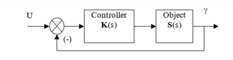
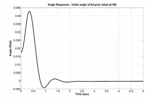
Simulating the control system using controller (8), the results are as follows Figure 3.
Figure 3. The angle response of bicycle robot
From Figure 3, it can be seen that: The dynamic quality indicators of the output response of the robot balance control system are:
•Number of oscillations: 04
•Maximum tilt angle: 0.43 rad
•Transition time: 2.25 s
With the initial tilt angle of the robot being pi/180 rad, after 4 oscillations, the control system has returned the tilt angle of the robot to 0 rad. Thus, the original controller is capable of maintaining the robot's stable balance.
However, the 6th-order controller (original controller) will lead to many disadvantages, such as a complicated control program and increased response time of the system, and can make the system unstable. Therefore, to improve the quality of the control system, the authors need to simplify the original controller so that the control program is simple, reducing the system's response time while still satisfying the stable and sustainable requirements of the system.
There have been many model reduction algorithms proposed to solve the model reduction problem. However, in the author's opinion, the "best" model reduction algorithm, i.e. the algorithm that meets all the requirements of the reduction problem in general and the controller reduction problem in particular, has not yet appeared. Each model reduction algorithm has its own advantages and disadvantages and its own scope of application. Therefore, to find a controller to replace the high-order controller, it is necessary to evaluate and compare the low-order controllers obtained by different model order reduction methods both in simulation and experiment.
Truncation techniques are applied when the system is in equilibrium representation to retain the states with large Hankel singular values in the reduced order system. The balance truncation algorithm (BTA) [18-20] performed a simultaneous crossover of the controllability and observability Gramians of the original system, thereby bringing the original system to the equilibrium representation. The truncation technique is used to retain large Hankel singular values in the low-order system. The BTA algorithm is introduced in detail in reference [18].
The optimal Hankel norm approximation (OHNA) [21-23] performs calculations to determine the optimal approximate order reduction system based on approximating the optimal Hankel singular value without bringing the original system to equilibrium representation. The OHNA algorithm is introduced in detail in reference [21].
The algorithm based on preserving dominant poles (PDP) [24, 25] will transform the original system to the upper triangular form. Then, the dominant points will be sorted according to the descending dominant index on the main diagonal of the A matrix of the system. The truncation technique is used to retain the poles with a large dominant index in the low-order system. The PDP algorithm is introduced in detail in reference [24].
The balance truncation algorithm [18-20], the optimal Hankel norm approximation [21-23], and the algorithm based on PDP [24-26] are considered popular order reduction algorithms. Therefore, in this study, the authors will use the above three algorithms to simplify the 6th-order robust controller (the original system).
Performing order reduction of the original system according to the order reduction algorithms, the results obtained in Tables 2-4.
The reduced order error values in Tables 2-4 are determined by the H¥ norm of the error transfer function, which is the difference between the transfer function of the original system and the transfer function of the corresponding reduced order system.
Table 2. The low-order controllers obtained by the BTA
|
Order |
The Low-Order Controller Kr(s) |
Error $\left\|\boldsymbol{K}-\boldsymbol{K}_r\right\|_{\infty}$ |
|
3 |
$\frac{-2.42310^4 s^2+3.311 .10^4 s+8264}{s^3+93.49 s^2+1749 s+338.2}$ |
8.0348.10-4 |
|
2 |
$\frac{-2.423 .10^4 s+3.797 .10^4}{s^2+93.29 s+1730}$ |
2.4868 |
|
1 |
$\frac{8.581}{s+0.03045}$ |
257.399 |
Table 3. The low-order controllers obtained by the OHNA
|
Order |
The Low-Order Controller Kr(s) |
Error $\left\|\boldsymbol{K}-\boldsymbol{K}_r\right\|_{\infty}$ |
|
3 |
$\frac{-2.42310^4 s^2+3.31 .10^4 s+8269}{s^3+93.49 s^2+1749 s+338.4}$ |
7.9387.10-4 |
|
2 |
$\frac{-2.47 .10^4 s+3.802 .10^4}{s^2+95.1 s+1732}$ |
2.4869 |
|
1 |
$\frac{211.5}{s+0.746}$ |
259.03 |
Table 4. The low-order controllers obtained by the algorithm based on PDP
|
Order |
The Low-Order Controller Kr(s) |
Error $\left\|\boldsymbol{K}-\boldsymbol{K}_r\right\|_{\infty}$ |
|
3 |
$\frac{-2.42310^4 s^2+3.299 .10^4 s+8447}{s^3+93.49 s^2+1749 s+346.1}$ |
0.0286 |
|
2 |
$\frac{-6334 s+1474}{s^2+25.74 s+5.108}$ |
264.1099 |
|
1 |
$\frac{-6227}{s+25.54}$ |
268.2455 |
Controllers are usually evaluated through transient response and frequency response. A low-order controller that wants to replace the original controller needs to preserve the transient and frequency characteristics of the original controller. Therefore, in addition to the basis of the order reduction error value in Tables 2-4, we compare the transient response and frequency response of low-order controllers and the original controller, the results are shown in Figure 4 and Figure 5.
(a) The step response of the 1st-order controllers
(b) The step response of the 2nd-order controllers
(c) The step response of the 3rd-order controllers
Figure 4. The comparison results of the step response of the controllers
(a) The frequency diagram of the 2nd-order controllers
(b) The frequency diagram of the 3rd-order controllers
Figure 5. The comparison results of the frequency diagram of the controllers
From Figures 4 and 5 and Tables 2-4, it is shown that:
•The responses of the 3rd-order controllers coincide with those of the original controller;
•The deviation between the response of the second-order controller, obtained by BTA and OHNA, and the response of the original system is very small.
•The responses of the 1st-order controller and the 2nd-order controller, obtained by the algorithm based on PDP, has a significant error compared to the responses of the sixth order controller.
The suitable low-order controller to replace the original controller must satisfy the criteria such as the lowest possible controller order and the smallest possible order reduction error. The third-order controller has a small order reduction error but has a higher order than the second-order controller. Therefore, the most suitable lower-order controller to replace the original controller is the second-order controller.
In which, the 2nd-order controller, obtained by the BTA, has a smaller order reduction error than the 2nd-order controller obtained by OHNA. Therefore, the second-order controller, obtained from BTA, is the most suitable low-order controller to replace the original controller.
To clarify the substitutability of the second-order controller for the original controller in the bicycle robot balancing control system, in this part, the author will simulate the bicycle robot balance control system using the 2nd-order controller, obtained by BTA and the original controller.
On the other hand, to get more information about the influence of the linearization process of the bicycle robot mathematical model on the quality of the bicycle robot balance control system, we perform simulations in the following 2 cases.
Case 1: Using the linear mathematical model of the bicycle robot. The initial assumption is that the bicycle robot deviates from the equilibrium position with the tilt angle $\theta=\frac{\pi}{180}(\mathrm{rad})$ and $\theta=\frac{\pi}{4}(\mathrm{rad})$. The simulation results of the bicycle robot balance control system when the robot initially deviates from the vertical at an angle $\theta=\frac{\pi}{180}(\mathrm{rad})$ and $\theta=\frac{\pi}{4}(\mathrm{rad})$ is shown in Figure 6.
(a) The angle of the robot when the robot initially deviates from the vertical at an angle $\theta=\frac{\pi}{180}(\mathrm{rad})$
(b) The angle of the robot when the robot initially deviates from the vertical at an angle $\theta=\frac{\pi}{4}(\mathrm{rad})$
Figure 6. The angle of the robot when using the linear robot model
Comment: From Figure 6(a), it can be seen that: The dynamic quality indicators of the output response of the robot balance control system are:
•Number of oscillations: 04
•Maximum tilt angle: 1.8 rad
•Transition time: 2.25 seconds
With the initial tilt angle of the robot being pi/180 rad, after 4 oscillations, the bicycle robot balance control system has brought the robot back to the equilibrium position (the robot's tilt angle is equal 0).
From Figure 6(b), it can be seen that: The dynamic quality indicators of the robot balance control system are:
•Number of oscillations: 04
•Maximum tilt angle: 0.43 rad
•Transition time: 2.25 seconds
With the initial tilt angle of the robot being pi/4 rad, after 4 oscillations, the bicycle robot balance control system has brought the robot back to the equilibrium position (the robot's tilt angle is equal 0).
When using the linear model of the robot, the second order controller can maintain the robot's equilibrium with a large initial robot tilt angle.
Case 2: Using the nonlinear mathematical model of the bicycle robot. The initial assumption is that the bicycle robot deviates from the equilibrium position with tilt angles $\theta=\frac{\pi}{180}(\mathrm{rad})$, $\theta=\frac{1.5 \pi}{180}(\mathrm{rad})$ and $\theta=\frac{2 \pi}{180}(\mathrm{rad})$. The simulation results of the bicycle robot balance control system when the robot initially deviates from the vertical at an angle $\theta=\frac{\pi}{180}(\mathrm{rad})$ , $\theta=\frac{1.5 \pi}{180}(\mathrm{rad})$ and $\theta=\frac{2 \pi}{180}(\mathrm{rad})$ is shown in Figure 7.
(a) The angle of the robot when the robot initially deviates from the vertical at an angle $\theta=\frac{\pi}{180}(\mathrm{rad})$
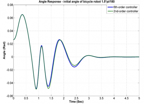
(b) The angle of the robot when the robot initially deviates from the vertical at an angle $\theta=\frac{1.5 \pi}{180}(\mathrm{rad})$
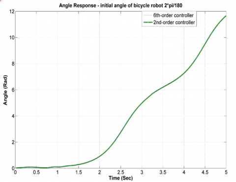
(c) The angle of the robot when the robot initially deviates from the vertical at an angle $\theta=\frac{2 \pi}{180}(\mathrm{rad})$
Figure 7. The angle of the robot when using the nonlinear robot model
Comment: From Figure 7(a), it can be seen that: The dynamic quality indicators of the output response of the robot balance control system are:
•Number of oscillations: 04
•Maximum tilt angle: 0.43 rad
•Transition time: 2.25 seconds
With the initial tilt angle of the robot being pi/180 rad, after 4 oscillations, the bicycle robot balance control system has brought the robot back to the equilibrium position (the robot's tilt angle is equal 0).
From Figure 7(b), it can be seen that: The dynamic quality indicators of the robot balance control system are:
•Number of oscillations: 04
•Maximum tilt angle: 0.65 rad
•Transition time: 3.25 seconds
With the initial tilt angle of the robot being 1.5*pi/180 rad, after 7 oscillations, the bicycle robot balance control system has brought the robot back to the equilibrium position (the robot's tilt angle is equal to 0).
From Figure 7(c), it can be seen that: With the initial tilt angle of the robot being 2*pi/180 rad, the robot balance control system cannot bring the robot back to balance (i.e., the robot will fall over).
When using the 2nd-order controller, the system can maintain the robot balance when the robot deviates from the equilibrium stand with a small angle. When the robot deviates from the equilibrium stand with a large angle ($\theta>\frac{1.5 \pi}{180}(\mathrm{rad})$), the system using the original and the 2nd-order controller cannot maintain the robot’s balance.
The design of the 6th-order controller is based on the linear model of the two-wheeled robot with the condition of small tilt angle ($\theta \approx \varphi \leq 1.5^{\circ}$- corresponding to $2^* \mathrm{pi} / 180$ rad, then $\sin \theta=\sin \varphi \approx 0$). When using the linear model of the bicycle robot, the estimated tilt angle value of the controller and the tilt angle value calculated from the linear model completely match, so the control system will create a moment with enough value and in time to balance with the moment of gravity of the robot, thereby maintaining stable balance of the robot. Therefore, when changing the tilt angle value to the value $\theta$=45° (beyond the linear condition of the tilt angle), the robot is still able to balance stably.
When using the nonlinear model of the bicycle robot, with a small tilt angle ($\theta \approx \varphi \leq 1.5^{\circ}$- linear condition of the tilt angle), the estimated tilt angle value of the controller and the tilt angle value calculated from the nonlinear model have a small deviation, so the control system will still create a moment with enough value and in time to balance with the moment of gravity of the robot, thereby maintaining stable balance of the robot.
When using the nonlinear model of the bicycle robot, with a large tilt angle ($\theta \approx \varphi>1.5^{\circ}$- the linearization condition of the robot model is not guaranteed), the estimated tilt angle value of the controller with the calculated tilt angle value from the nonlinear model has a large deviation. Because of this reason, the control system will not be able to generate a sufficiently large and timely moment value to balance the robot's gravity moment, so the robot cannot maintain stable balance.
Thus, the control system using the controller designed based on the linear model of the bicycle robot model is only capable of maintaining stable balance of the bicycle robot when the tilt angle of the robot must be within the limit of the tilt angle ($\theta \approx \varphi \leq 1.5^{\circ}$), or the condition of linearization of the model is guaranteed.
The central controller of the bicycle robot model usually uses a microcontroller, so the controller of the robot control system will be written in the form of program code. In fact, compared with the program code of the 6th order controller, the program code of the 2nd order controller will be simpler and shorter, which will help reduce the processing time of the controller, thereby helping to reduce the response time of the control system.
The design of a robust controller for the balance control problem for a bicycle robot, based on the linear model of the bicycle robot, has obtained a 6th-order controller. In order to make the controller simpler while still maintaining the characteristics of a robust controller, the paper has applied some MOR algorithms to determine the low-order controllers from the 6th-order controller. At the same time, to compare and evaluate the low-order controllers, the paper has applied many different evaluation methods such as evaluation based on order reduction error, evaluation based on transient response and frequency response, evaluation based on transient response of the control system. Based on those evaluation results, the paper has selected the most suitable low-order controller to replace the 6th-order controller, these approaches of the paper can be applied to similar problems. On the other hand, the paper also points out the limitations of the controller (both low-order controller and 6th-order controller) when applied to the nonlinear model of the bicycle robot model. In the following studies, the author will compare and evaluate the low-order controller in the actual bicycle robot control system.
The authors gratefully acknowledge Thai Nguyen University of Technology, Vietnam, for supporting this work. This research was not affiliated with any funded scientific project.
|
A, B, C |
Matrix of the model |
|
S(s) |
Transfer function |
|
R |
DC motor resistance ($\Omega$) |
|
$\omega$ |
DC motor angular velocity (rad/s) |
|
$I_p$ |
The flywheel polar moment of inertia (Kg.m2) |
|
$I_r$ |
The flywheel radial moment of inertia (Kg.m2) |
|
$I_b$ |
The bicycle moment of inertia (Kg.m2) |
|
$h_b$ |
The height of bicycle center of gravity (m) |
|
$h_f$ |
The height of flywheel center of gravity (m) |
|
$m_g$ |
Bicycle masses (Kg) |
|
$m_f$ |
Flywheel masses (Kg) |
|
$K_e$ |
The back emf constants of the motor (V.s/Rad) |
|
$K_m$ |
The torque constants of the motor (Nm/A) |
|
$B_m$ |
The DC motor viscosity coefficient (Kg.m2/s) |
|
$\theta$ |
The angular velocity of the bicycle around Z axis (Rad) |
|
$\varphi$ |
The angular velocity of the flywheel around its control axis (X1 axis) (Rad) |
|
$T_m$ |
Torque generated by the motor (Kg.m2) |
|
U |
The input voltage to the DC motor (V) |
|
$g$ |
Free fall acceleration (m/s2) |
[1] Lee, S.I., Lee, I.W., Kim, M.S., He, H., Lee, J.M. (2012). Balancing and driving control of a bicycle robot. Journal of Institute of Control, Robotics and Systems, 18(6): 532-539. https://doi.org/10.5302/j.icros.2012.18.6.532
[2] Defoort, M., Murakami, T. (2009). Sliding-mode control scheme for an intelligent bicycle. IEEE Transactions on Industrial Electronics, 56(9): 3357-3368. https://doi.org/10.1109/TIE.2009.2017096
[3] Lot, R., Fleming, J. (2019). Gyroscopic stabilisers for powered two-wheeled vehicles. Vehicle System Dynamics, 57(9): 1381-1406. https://doi.org/10.1080/00423114.2018.1506588
[4] Park, S.H., Yi, S.Y. (2020). Active balancing control for unmanned bicycle using scissored-pair control moment gyroscope. International Journal of Control, Automation and Systems, 18(1): 217-224. https://doi.org/10.1007/s12555-018-0749-7
[5] Thanh, B.T., Parnichkun, M. (2008). Balancing control of bicyrobo by particle swarm optimization-based structure-specified mixed H2/H∞ control. International Journal of Advanced Robotic Systems, 5(4): 39. https://doi.org/10.5772/6235
[6] Bui, T.T., Parnichkun, M., Le, C.H. (2010). Structure-specified H∞ loop shaping control for balancing of bicycle robots: A particle swarm optimization approach. Proceedings of the Institution of Mechanical Engineers, Part I: Journal of Systems and Control Engineering, 224(7): 857-867. https://doi.org/10.1243/09596518JSCE950
[7] Kim, Y., Kim, H., Lee, J. (2015). Stable control of the bicycle robot on a curved path by using a reaction wheel. Journal of Mechanical Science and Technology, 29: 2219-2226. https://doi.org/10.1007/s12206-015-0442-1
[8] Kim, H.W., An, J.W., dong Yoo, H., Lee, J.M. (2013). Balancing control of bicycle robot using PID control. In 2013 13th International Conference on Control, Automation and Systems (ICCAS 2013), Gwangju, Korea (South), pp. 145-147. https://doi.org/10.1109/ICCAS.2013.6703879
[9] Kanjanawanishkul, K. (2015). LQR and MPC controller design and comparison for a stationary self-balancing bicycle robot with a reaction wheel. Kybernetika, 51(1): 173-191. https://doi.org/10.14736/kyb-2015-1-0173
[10] Vo, A.K., Nguyen, M.T., Nguyen, T.N., Van Nguyen, T., Doan, V.K., Tran, H.C., Nguyen, V.D.H. (2018). PD controller for bicycle model balancing. Robotica & Management, 23(2): 37-41.
[11] Chiu, C.H., Wu, C.Y. (2020). Bicycle robot balance control based on a robust intelligent controller. IEEE Access, 8: 84837-84849. https://doi.org/10.1109/ACCESS.2020.2992792
[12] Binh, N.H., Hung, V.D. (2023). Application of Zhou’s balanced truncation algorithm for controlling the balance of bicyrobot. Journal Européen des Systèmes Automatisés, 56(2): 231-236. https://doi.org/10.18280/jesa.560207
[13] Sikander, A., Prasad, R. (2019). Reduced order modelling based control of two wheeled mobile robot. Journal of Intelligent Manufacturing, 30: 1057-1067. https://doi.org/10.1007/s10845-017-1309-3
[14] Kien, V.N., Duy, N.T., Du, D.H., Huy, N.P., Quang, N.H. (2023). Robust optimal controller for two-wheel self-balancing vehicles using particle swarm optimization. International Journal of Mechanical Engineering and Robotics Research, 12(1): 16-22. https://doi.org/10.18178/ijmerr.12.1.16-22
[15] Tanaka, Y., Murakami, T. (2004). Self sustaining bicycle robot with steering controller. In the 8th IEEE International Workshop on Advanced Motion Control, Kawasaki, Japan, pp. 193-197. https://doi.org/10.1109/AMC.2004.1297665
[16] Huang, C.F., Tung, Y.C., Yeh, T.J. (2017). Balancing control of a robot bicycle with uncertain center of gravity. In 2017 IEEE International Conference on Robotics and Automation (ICRA), Singapore, pp. 5858-5863. https://doi.org/10.1109/ICRA.2017.7989689
[17] Glover, K., McFarlane, D. (1992). A loop shaping design procedure using H∞-synthesis. IEEE Transactions on Automatic Control, 37(6): 759-769. https://doi.org/10.1109/9.256330
[18] Moore, B. (1981). Principal component analysis in linear systems: Controllability, observability, and model reduction. IEEE Transactions on Automatic Control, 26(1): 17-32. https://doi.org/10.1109/TAC.1981.1102568
[19] Borghi, A., Breiten, T., Gugercin, S. (2025). Balanced truncation with conformal maps. Systems & Control Letters, 197: 106044. https://doi.org/10.1016/j.sysconle.2025.106044
[20] Benner, P., Goyal, P. (2024). Balanced truncation for quadratic-bilinear control systems. Advances in Computational Mathematics, 50: 88. https://doi.org/10.1007/s10444-024-10186-9
[21] Prajapati, A.K., Prasad, R. (2022). Model reduction using the balanced truncation method and the Padé approximation method. IETE Technical Review, 39(2): 257-269. https://doi.org/10.1080/02564602.2020.1842257
[22] Chui, C.K., Chen, G. (1997). Optimal hankel-norm approximation and H∞-minimization. In Discrete H∞ Optimization. Springer Series in Information Sciences. Springer, Berlin, Heidelberg. https://doi.org/10.1007/978-3-642-59145-7_4
[23] Safonov, M.G., Chiang, R.Y. (1988). A Schur method for balanced model reduction. In 1988 American Control Conference, Atlanta, GA, USA, pp. 1036-1040. https://doi.org/10.23919/ACC.1988.4789873
[24] Cao, X., Saltik, M.B., Weiland, S. (2018). Optimal Hankel norm approximation for continuous-time descriptor systems. In 2018 Annual American Control Conference (ACC), Milwaukee, WI, USA, pp. 6409-6414. https://doi.org/10.23919/ACC.2018.8431684
[25] Nguyen, C.H., Vu, K.N., Do, H.T. (2015). Model reduction based on triangle realization with pole retention. Applied Mathematical Sciences, 9(44): 2187-2196. https://doi.org/10.12988/ams.2015.5290
[26] Vu, N.K., Nguyen, H.Q. (2021). Model order reduction algorithm based on preserving dominant poles. International Journal of Control, Automation and Systems, 19(6): 2047-2058. https://doi.org/10.1007/s12555-019-0990-8