Fachri Faisal![]() | Henny Pramoedyo
| Henny Pramoedyo![]() | Suci Astutik*
| Suci Astutik*![]() | Achmad Efendi
| Achmad Efendi![]()
© 2025 The authors. This article is published by IIETA and is licensed under the CC BY 4.0 license (http://creativecommons.org/licenses/by/4.0/).
OPEN ACCESS
This research investigates the utilization of Bayesian Geographically Weighted Regression (BGWR) combined with Kriging to improve spatial predictions of the Human Development Index (HDI) throughout Sumatra Island. The results underscore considerable geographical variations in human development indicators, such as life expectancy, education, and economic measures. While the standard Geographically Weighted Regression (GWR) model produces reliable results, incorporating Bayesian frameworks—particularly with Jeffreys' uninformative prior—delivers superior predictive performance and effectively addresses spatial heterogeneity. The Bayesian Jeffreys model achieves the highest accuracy across multiple metrics, including the lowest mean absolute bias (MAB) and root mean squared error (RMSE), explaining 99.99% of HDI variance. Moreover, the Jeffreys model specifically reduces spatial autocorrelation in residuals, lowering the demand for further methods, including Kriging. By proving the superiority of Jeffreys' previous over conjugate priors in handling spatial heterogeneity and enhancing prediction accuracy, this work adds to the body of knowledge. It provides a strong basis for precision-driven spatial analyses in regional development planning and resource allocation. The results also highlight the urgent need for focused policy interventions to solve ongoing disparities in underdeveloped areas using metropolitan centers as scalable development models.
BGWR, Kriging, HDI, spatial prediction, Jeffreys’ prior, conjugate prior, spatial heterogeneity, spatial autocorrelation
The Human Development Index (HDI) is a comprehensive socio-economic development measure encompassing health, education, and income indicators. Understanding the spatial distribution of HDI is crucial for addressing regional disparities and designing targeted policies that foster sustainable development. On Sumatra Island, variations in HDI across districts and cities reflect disparities in life expectancy, educational attainment, and per capita income. Analyzing these spatial variations offers valuable insights into the factors driving development and identifies areas requiring targeted interventions.
Traditional regression models often struggle to account for the local spatial variations inherent in development indicators like HDI. Geographically Weighted Regression (GWR), introduced by the study [1], overcomes this limitation by allowing regression coefficients to vary spatially. However, GWR has limitations, including restrictive assumptions that compromise predictive accuracy and parameter stability. To address these shortcomings, Bayesian Geographically Weighted Regression (BGWR) extends GWR by incorporating hierarchical Bayesian inference. This approach stabilizes parameter estimation and reduces uncertainty by integrating prior knowledge. Nonetheless, residual spatial autocorrelation often persists, indicating the presence of unmodeled spatial dependencies.
Despite BGWR's advancements, two critical challenges remain underexplored in the existing literature: (1) the influence of prior choices (e.g., conjugate priors versus Jeffreys' uninformative priors) on prediction accuracy and parameter stability, and (2) the persistent issue of residual spatial dependencies. Addressing these gaps is essential for improving the robustness and reliability of spatial modeling in HDI analysis.
This study introduces a hybrid approach integrating BGWR with Kriging to address these challenges. Kriging, a geostatistical interpolation method designed explicitly for spatially autocorrelated data, enhances spatial predictions by capturing residual spatial dependencies, especially in regions with sparse data or complex spatial structures. The proposed BGWR-Kriging framework combines BGWR's capacity to model local variation with Kriging's strength in addressing unmodeled spatial dependencies, enhancing predictive accuracy. Recent studies [2-7] have demonstrated the utility of hybrid methods like GWR-Kriging in spatial modeling; however, their application to HDI analysis remains unexplored.
This study also makes a novel contribution by comparing the performance of conjugate priors, known for their mathematical convenience [8], with Jeffreys' uninformative priors, which are invariant under parameter transformations [9-11]. Such a comparison is vital, as the prior choice directly impacts prediction accuracy and parameter stability in spatial modeling.
This study addresses existing research gaps by applying the hybrid BGWR-Kriging approach to HDI data from Sumatra Island. It offers a robust framework for the spatial analysis of socio-economic indicators. The findings are expected to inform policies to reduce regional disparities and promote equitable development, with practical implications for urban planning, education, and healthcare resource allocation.
Furthermore, this study deliberately compares conjugate and Jeffreys' priors to represent two contrasting Bayesian approaches in spatial modeling. Conjugate priors are selected for their computational convenience, enabling efficient estimation in large spatial datasets. In contrast, Jeffreys' prior, which is uninformative and invariant under parameter transformations, is particularly valuable in contexts with limited prior information regarding spatial processes, such as HDI modeling across diverse geographic regions. By comparing these priors within the BGWR framework, this study aims to assess the trade-off between computational tractability and estimation flexibility, offering practical insights into prior selection for spatial modeling.
2.1 Bayesian inference
Bayesian inference combines observed data with prior knowledge to derive posterior distributions, allowing for robust parameter estimation, particularly in spatial data where variability and uncertainty are prevalent. This approach relies on three key components: prior distributions, which incorporate pre-existing assumptions about model parameters based on prior studies or reasonable expectations; the likelihood function, which quantifies the probability of observed data given the model parameters; and posterior distributions, which update prior beliefs with observed data to produce refined parameter estimates. Bayes’ theorem was applied as:
$f(\theta \mid y) \propto f(y \mid \theta) f(\theta)$ (1)
where, $f(\theta \mid y)$ is the posterior distribution, $(y \mid \theta)$ is the likelihood, and $f(\theta)$ is the prior [12].
This research employed two types of priors for comparative purposes: conjugate priors and Jeffreys' prior. The conjugate prior was utilized due to its analytical tractability, facilitating closed-form solutions and enhancing computational efficiency. It is essential in processing extensive spatial datasets such as the HDI across Sumatra Island. Meanwhile, Jeffreys' prior was adopted for its uninformative nature and invariance under parameter reparameterization, providing neutrality and robustness, especially when prior information regarding spatial dependencies is limited or unknown. Through this dual-prior approach, the study aims to evaluate how prior choice affects parameter stability, spatial heterogeneity capture, and predictive accuracy within the BGWR framework.
2.2 GWR model structure
The core function of GWR is to model spatial heterogeneity by allowing regression coefficients to vary across locations. It builds upon the ordinary least squares (OLS) regression but introduces spatial weighting to capture local variations. The formula is structured as follows:
$y_i=\beta_0\left(u_i, v_i\right)+\sum_{k=1}^p \beta_k\left(u_i, v_i\right) x_{i k}+\epsilon_i$ (2)
In this study, let $y_i$ denote the response variable at location i, where the geographic coordinates of location i are represented by ($u_i, v_i$). The model incorporates $x_{ik}$ as the k predictor variables, each associated with a location-specific regression coefficient $\beta_k\left(u_i, v_i\right) x_{i k}$, allowing for spatially varying relationships. The term $\epsilon_i$ represents the error component, capturing the unexplained variability in the response variable.
GWR uses spatially varying coefficients to reflect the influence of local contexts on the relationship between predictors and the response. These coefficients are estimated through weighted least squares, where weights are determined based on the distance between observed points. GWR is beneficial for data with strong local dependencies, as in environmental, socioeconomic, or epidemiological studies [13, 14].
The choice of bandwidth, which defines the spatial scale of the analysis, is essential in GWR. Bandwidth determines the neighborhood size over which local coefficients are calculated, affecting how much the surrounding data influences each local model. There are two approaches to the bandwidth selection process: fixed and adaptive. Fixed bandwidth is a constant bandwidth across the entire study area and is, therefore, appropriate for data with uniformly dispersed observations. On the other hand, adaptive bandwidth is a variable bandwidth that depends on the level of observation density, so it is more flexible in modeling spatially heterogeneous data by tuning the bandwidth according to the local data distribution.
Bandwidth selection is often optimized by minimizing a criterion, such as the Akaike Information Criterion (AIC) or cross-validation score. Once selected, the spatial weight matrix $W_i$ is constructed, where each element $w_{ij}$ represents the weight between locations i and j. A common approach for determining weights is the Gaussian function:
$w_{i j}=\exp \left(-\frac{d_{i j}^2}{2 b^2}\right)$ (3)
where, $d_{i j}$ is the distance between locations i and j, and b is the bandwidth parameter. This weighted matrix plays a critical role in producing locally varying parameter estimates, balancing the trade-off between model flexibility and stability [15, 16].
This study adopted a fixed bandwidth approach using a Gaussian kernel to ensure consistent local regression scales across Sumatra Island. This approach was considered appropriate given the moderate spatial heterogeneity of the HDI data, which did not exhibit extreme clustering or sparsity that would require an adaptive approach. The optimal bandwidth was selected to minimize the model predictions' mean squared error (MSE), which emphasizes reducing prediction errors across locations. The use of MSE as the optimization criterion aligns with the predictive objective of this study and is recognized as a valid method for bandwidth selection in GWR applications. Furthermore, adopting a fixed bandwidth facilitates the interpretability and comparability of local parameter estimates across regions.
2.3 BGWR
The BGWR model combines the strengths of Bayesian inference with the flexibility of GWR. This approach incorporates uncertainty in spatially varying coefficients while addressing the heterogeneity of socioeconomic data. The likelihood for the BGWR model is given by [17]:
$\mathbf{Y} \mid \boldsymbol{\beta}(\mathbf{s}), \mathbf{X}, \mathbf{W}(\mathbf{s}), \sigma^2(s) \sim M V N\left(\mathbf{X} \boldsymbol{\beta}(\mathbf{s}), \sigma^2(s) \mathbf{W}^{-\mathbf{1}}(\mathbf{s})\right)$ (4)
Here, $\mathbf{Y}$ represents the vector of observed responses, while $\boldsymbol{\beta}(\mathbf{s})$ denotes the spatially varying regression coefficients that capture local relationships between predictors and the response variable. The predictor variables are organized in the matrix $\mathbf{X}$, with spatial dependencies incorporated through the spatial weight matrix $\mathbf{W}(\mathbf{s})$, which adjusts the influence of nearby observations. Finally, $\sigma^2(s)$ represents the spatially varying variance, allowing the model to account for heteroscedasticity and location-specific uncertainties.
Posterior distributions were derived for coefficients and variance using Conjugate [17] and Jeffreys’ priors [18]. The following are the marginal posterior distributions for Conjugate prior for $\boldsymbol{\beta}(\mathbf{s})$ and $\sigma^2(s)$:
$\boldsymbol{\beta}(\mathbf{s}) \mid \mathbf{Y}, \sigma^2(s) \sim M V N(\mu, \Lambda)$ (5)
Here, $\mu=\Lambda^{-1} X^T W(s) Y$ represents the posterior mean, which provides an estimate of the spatially varying regression coefficients based on the observed data. The term $\Lambda=\frac{1}{\sigma^2(s)}\left(X^T W(s) X+\Sigma_\beta^{-1}\right)$ defines the precision matrix, which controls the variability of the posterior distribution. Within this expression, $\Sigma_\beta^{-1}$ represents the prior covariance matrix for $\boldsymbol{\beta}(\mathbf{s})$ incorporating prior information to regularize the estimation of spatially varying coefficients.
The marginal posterior for $\sigma^2(s)$ follows an inverse gamma distribution:
$\sigma^2(s) \mid \mathbf{Y} \sim {IG}\left(\alpha^{\prime}, \alpha_1^{\prime}\right)$, (6)
$\alpha^{\prime}=\alpha_0+\frac{n}{2}, \alpha_1^{\prime}=\alpha_1+\frac{1}{2}\left(Y^T W(s) Y-\mu^T \Lambda \mu\right)$ (7)
The following are the marginal posterior distributions for Jeffreys’ prior for $\boldsymbol{\beta}(\mathbf{s})$ and $\sigma^2(s)$:
$\boldsymbol{\beta}(s) \mid \mathbf{Y}, \sigma^2(s) \sim M V N\left(\beta_0, \sigma^2(s)\left(X^T W(s) X\right)^{-1}\right)$ (8)
Here, the posterior mean of the regression coefficients is given by $\beta_0=\left(X^T W(s) X\right)^{-1} X^T W(s) Y$, which represents the weighted least squares estimate incorporating spatial weighting. The covariance matrix of the posterior distribution is expressed as $\sigma^2(s)\left(X^T W(s) X\right)^{-1}$, capturing the uncertainty in the estimated coefficients while accounting for spatial variability.
The marginal posterior $\sigma^2(s)$ for Jeffreys’ prior follows an inverse gamma distribution:
$\sigma^2(s) \left\lvert\, \mathbf{Y} \sim I G\left(\frac{n+1}{2}, \frac{Y^T W(s) Y-Y^T X\left(X^T W(s) X\right)^{-1} X^T W(s) Y}{2}\right)\right.$ (9)
where, n is the number of observations.
A leave-one-out cross-validation (LOOCV) strategy was implemented to assess the model's out-of-sample predictive performance. The Bayesian GWR model was re-estimated for each observation using the remaining data, excluding the target point. Predictions for the excluded locations were generated using the local regression coefficients derived from the training subset. Due to the lack of a direct Bayesian implementation for LOOCV with Jeffreys' prior, the procedure employed GWR as a frequentist analog, which retains the same spatial prediction structure. This approach provides a reliable estimation of generalization performance while maintaining methodological consistency with the original model [19-21].
2.4 Kriging of residuals
After estimating the BGWR model, the residuals $\epsilon_i$ are calculated as:
$\epsilon_i=Y_i-\widehat{Y}_i$, (10)
where, $\widehat{Y}_i$ is the predicted value from the BGWR model. These residuals are then kriged to account for spatial autocorrelation that remains unaddressed in the GWR model. The Kriging estimator is:
$\hat{Z}(s)=\sum_{i=1}^n \lambda_i \epsilon_i$ (11)
Here, $\hat{Z}(s)$ represents the estimated residual at an unsampled location s, obtained through Kriging interpolation. The term $\lambda_i$ denotes the weights assigned to each sampled location, which are determined based on the spatial correlation structure of the residuals. Finally, n refers to the number of sampled locations, influencing the Kriging estimation process and the accuracy of spatial predictions [22].
The semivariogram used for Kriging is defined as:
$\gamma(h)=\frac{1}{2 N(h)} \sum_{i=1}^{N(h)}\left[\epsilon\left(s_i\right)-\epsilon\left(s_i+h\right)\right]^2$ (12)
$\gamma(h)$ represents the semivariance at a given lag distance h, quantifying the spatial dependence between observations. $N(h)$ denotes the number of observation pairs separated by distance h, influencing the reliability of the semivariance estimate. Lastly, $\epsilon\left(s_i\right)$ corresponds to the residual value at location $s_i$, capturing the unexplained variation in the spatial model [23, 24].
Three theoretical semivariogram models—Spherical, Exponential, and Gaussian—were fitted to the empirical semivariogram. The LOOCV method was adopted to ensure rigorous model selection. LOOCV is widely accepted in geostatistics for evaluating spatial interpolation models, as it provides an unbiased estimate of predictive performance by systematically leaving out each data point during model training and assessing the accuracy of the prediction for that point. Recent literature has emphasized this method as a reliable approach to evaluate model generalizability and mitigate overfitting in spatial modeling frameworks [25, 26]. The semivariogram model with the lowest mean squared prediction error (MSPE) from the LOOCV procedure was selected for further Kriging implementation. For each model, the parameters (nugget, sill, and range) were estimated using an iterative weighted least squares (WLS) fitting procedure based on the empirical semivariogram.
2.5 Combining BGWR and Kriging
The final prediction from BGWRK is obtained by combining the predictions from the GWR model with the kriged residuals:
$\hat{Y}_{B G W R K}(s)=\hat{Y}(s)+\hat{Z}(s)$ (13)
Here, $\hat{Y}_{B G W R K}(s)$ represents the final prediction at location sss, obtained by integrating BGWRK. The term $\hat{Y}(s)$ denotes the prediction from the BGWR model, capturing spatially varying relationships between predictors and the response variable. Lastly, $\hat{Z}(s)$ corresponds to the kriged residual at location $s$, which accounts for spatially structured errors and enhances prediction accuracy [27].
2.6 Study area and data sources
This study investigates spatial disparities in human development by analyzing the HDI across 154 districts and cities on the island of Sumatra, Indonesia. Sumatra was selected due to its diverse socioeconomic characteristics, which provide a robust foundation for evaluating spatial variability in development outcomes.
The secondary data for the HDI in 2021 were obtained from the Central Bureau of Statistics (BPS) [28]. Data validation was performed by cross-referencing independent regional reports to ensure consistency and reliability. The dataset comprises variables aligned with the HDI dimensions. The response variable ($Y$) is the HDI, representing the HDI values for districts and cities in Sumatra for the year 2021. The predictor variables ($X$) include Life Expectancy at Birth ($X_1$), which measures the average number of years a newborn is expected to live under prevailing mortality rates, representing the health dimension; Expected Years of Schooling ($X_2$), indicating the number of years a child entering school is expected to spend in formal education, reflecting future educational attainment; Mean Years of Schooling ($X_3$), capturing the average years of schooling completed by individuals aged 25 and older, representing historical education levels; and Adjusted Per Capita Expenditure ($X_4$), which reflects the standard of living by accounting for average per capita spending adjusted for regional cost-of-living differences.
2.7 Research steps
This study uses advanced spatial modeling techniques to analyze the spatial variability of the HDI across Sumatra Island, Indonesia. By integrating GWR, Bayesian inference, and Kriging, the methodology aims to capture local variations and address spatial autocorrelation in the data. Below, the research steps are outlined, from data collection to model evaluation and interpretation.
1) Data Collection: This study focuses on Sumatra Island, analyzing HDI data from 154 districts and cities in 2021, which were sourced from BPS and validated with independent reports.
2) Exploratory Data Analysis: Descriptive statistics and spatial visualizations were used to assess the data. Moran’s I test confirmed spatial clustering, justifying the need for geographically adaptive modeling.
3) Model Building and Selection: GWR was initially applied to capture local variations in HDI predictors. To enhance accuracy, BGWR was used, incorporating Conjugate Priors for efficiency and Jeffreys’ Uninformative Priors for robustness. MCMC methods were employed for parameter estimation.
4) Residual Analysis and Kriging: Residual spatial autocorrelation was identified through the Moran’s I test, prompting using Kriging for spatial interpolation. Several theoretical semivariogram models were evaluated, and the optimal model was selected based on leave-one-out cross-validation (LOOCV) to improve the prediction accuracy.
5) Model Evaluation and Comparison: Performance was assessed using MAB, MSD, RMSE, and R², identifying the Bayesian Jeffreys model as the most accurate in capturing spatial variability.
6) Visualization and Interpretation: Spatial maps illustrated HDI disparities across Sumatra, highlighting well-developed urban centers like Pekanbaru and Medan, while rural areas such as Nias and Simeulue showed lower HDI. These insights provide valuable input for policy and resource allocation.
The analysis provides a detailed overview of key human development indicators for 154 districts and cities across Sumatra Island. These metrics include the HDI, life expectancy at birth, education-related measures, and economic indicators, summarized in Table 1.
Table 1. Descriptive statistics of human development indicators across Sumatra
|
Metric |
HDI |
Life Expectancy at Birth |
Expected Years of Schooling |
Mean Years of Schooling |
Adjusted Per Capita Expenditure |
|
Count |
154 |
154 |
154 |
154 |
154 |
|
Mean |
71.03 |
69.19 |
13.28 |
8.87 |
10,576.22 |
|
Median |
70.11 |
69.26 |
13.06 |
8.63 |
10,384.50 |
|
Standard Deviation |
4.54 |
2.40 |
1.06 |
1.34 |
2,041.49 |
|
Minimum |
61.99 |
62.39 |
11.38 |
5.64 |
5,924.00 |
|
Maximum |
85.71 |
74.50 |
17.80 |
12.83 |
18,034.00 |
The HDI averages 71.03 (±4.54 SD) across the regions, ranging from 61.99 in Nias Selatan to 85.71 in Pekanbaru. Such areas as Pekanbaru and Medan exhibit high HDI values, signifying advanced development levels, while districts such as Nias Selatan, Simeulue, and Aceh Singkil show lower HDI scores, highlighting disparities in regional development.
Life Expectancy at Birth averages 69.19 years (±2.40 SD), ranging from 62.39 years in Nias to 74.50 years in Tapanuli Selatan. Cities such as Banda Aceh and Padang Panjang report higher life expectancy values, reflecting better healthcare and living conditions. In contrast, rural districts like Nias and Mandailing Natal have significantly lower life expectancy.
Expected Years of Schooling across Sumatra regions show a mean of 13.28 years (±1.06 SD). Urban centers such as Medan, Palembang, and Banda Aceh report expected years of schooling exceeding 14 years, while rural districts, including Nias and Padang Lawas Utara, lag with averages below 12 years. The Mean Years of Schooling reflects a similar trend, with an average of 8.87 years (±1.34 SD). Medan and Banda Aceh report over 10 years of mean schooling, while regions like Nias Selatan and Aceh Tenggara fall below 7 years.
Economic indicators, represented by Adjusted Per Capita Expenditure, average IDR 10,576.22 thousand (±IDR 2,041.49 thousand SD), ranging from IDR 5,924.00 thousand in Nias Barat to IDR 18,034.00 thousand in Batam. Urbanized and industrialized regions such as Batam, Pekanbaru, and Medan show significantly higher per capita expenditures. In contrast, rural districts in Aceh and Nias regions exhibit lower averages, pointing to economic inequalities.
The results highlight significant variability in human development across Sumatra Island. Urban centers such as Pekanbaru, Batam, and Medan consistently perform better across multiple indicators, reflecting concentrated infrastructure, healthcare access, and economic opportunities. Conversely, districts in Nias and rural Aceh face systemic challenges, with lower HDI, limited educational attainment, and reduced economic output.
These findings emphasize the critical need for targeted interventions to address disparities in underperforming regions such as Nias Selatan, Simeulue, and Aceh Singkil, particularly in education and economic development. Conversely, leveraging the strengths of high-performing urban centers may provide scalable models for regional development across Sumatra.
Before employing GWR, it is crucial to establish the presence of spatial heterogeneity in the data. Spatial heterogeneity refers to inconsistent relationships between independent and dependent variables across the entire geographic area. Moran's I [29] or the Local Indicator of Spatial Association (LISA) frequently detects spatial patterns within the data. Without spatial heterogeneity, using a global regression model may be more appropriate [30].
The Moran's I test was applied to analyze the spatial clustering of residuals from the regression model, aiming to detect whether spatial patterns exist in the dataset. The results of Moran's I test for the global regression residuals reveal the following in Table 2.
Table 2. Results of the Moran's I test
|
Statistic |
Value |
|
Moran's I Statistic |
0.501 |
|
Expectation |
−0.0065 |
|
Variance |
0.0018 |
|
Z-Score (Standard Deviate) |
12.023 |
|
p-value |
< 2.2 × 10⁻¹⁶ |
These results indicate a statistically significant positive spatial autocorrelation of the residuals at a very high confidence level (p-value < 0.001). The Moran's I value of 0.501 suggests a moderate to strong clustering of similar residual values across the geographic units of analysis (Sumatra). The expectation value close to zero indicates that the null hypothesis assumes no spatial autocorrelation, while the very high Z-score confirms that the observed clustering is not random. The Moran's I test results show significant positive spatial autocorrelation in the residuals of the global regression model. This implies that the relationships between the dependent variable HDI and the independent variables (Life Expectancy at Birth, Expected Years of Schooling, Mean Years of Schooling, and Adjusted Per Capita Expenditure) are not fully captured by the global regression model. The clustering of residuals suggests that spatially varying relationships are present in the data.
This study seeks to understand the relationships between the dependent variable and the predictors through global and local perspectives. A global regression approach provides a single set of parameter estimates applicable across the study area. In contrast, GWR allows for spatially varying coefficients, offering more profound insights into localized patterns of association. Before conducting Bayesian model estimation, we summarize the findings of the global regression model and the local parameter estimates derived from GWR in Tables 3 and 4, respectively. These results establish a foundation for understanding the variability in the data and provide benchmarks for comparison with the subsequent Bayesian model.
Table 3. Global parameter estimation
|
Parameter |
Coefficients |
Std. Error |
p-value |
|
Intercept |
4.6650 |
1.1730 |
0.000109 |
|
$X_1$ |
0.4889 |
0.01721 |
< 2 × 10-16 |
|
$X_2$ |
0.8579 |
0.05211 |
< 2 × 10-16 |
|
$X_3$ |
1.2990 |
0.04981 |
< 2 × 10-16 |
|
$X_4$ |
0.0009105 |
0.00002259 |
< 2 × 10-16 |
Table 4. Summary of local parameter estimation for GWR
|
Parameter |
Min |
Max |
Mean |
Stdev |
|
$\beta_0$ |
4.544712968 |
4.751145608 |
4.634841874 |
0.056078583 |
|
$\beta_1$ |
0.488548980 |
0.489289201 |
0.488875315 |
0.000156652 |
|
$\beta_2$ |
0.848324734 |
0.871484688 |
0.860929239 |
0.006232544 |
|
$\beta_3$ |
1.293265767 |
1.301612298 |
1.297090946 |
0.002287895 |
|
$\beta_4$ |
0.000906908 |
0.000914278 |
0.000911312 |
1.57839×10⁻⁶ |
Table 3 summarizes the global parameter estimation results derived from the regression analysis. The intercept is estimated at 4.665 with a standard error of 1.173, and its associated p-value of 0.000109 indicates strong statistical significance. Among the independent variables, $X_1$, $X_2$, $X_3$, and $X_4$ demonstrate highly significant effects on the dependent variable, with p-values less than $2 \times 10^{-16}$. Specifically, the coefficient for $X_1$ is 0.4889 (Std. Error: 0.01721), for $X_2$ is 0.8579 (Std. Error: 0.05211), for $X_3$ is 1.299 (Std. Error: 0.04981), and for $X_4$ is 0.0009105 (Std. Error: 0.00002259). These findings suggest that all predictors significantly contribute to explaining variations in the response variable, with $X_3$ showing the most significant magnitude of effect among the predictors.
Table 4 presents the summary statistics of the GWR local parameter estimates. The intercept ($\beta_0$) exhibits a mean value of 4.6348 with a standard deviation (Stdev) of 0.0561, ranging from 4.5447 to 4.7511 across the spatial units. The local estimates for $\beta_1$ demonstrate minimal variability, with a mean of 0.4889, a standard deviation 0.0002, and a narrow range between 0.4885 and 0.4893. For $\beta_2$, the mean value is 0.8609 with a standard deviation of 0.0062, which varies between 0.8483 and 0.8715. Similarly, $\beta_3$ displays a mean of 1.2971, a standard deviation of 0.0023, and a range from 1.2933 to 1.3016. Finally, $\beta_4$ demonstrates the least variability, with a mean of 0.0009113, a standard deviation of 0.0000016, and a range of 0.0009069 to 0.0009143.
These results indicate substantial spatial variation in the local parameter estimates, particularly for $\beta_2$ and $\beta_3$, highlighting potential regional differences in the predictors' influence. The relatively low variability observed in $\beta_1$ and $\beta_4$ suggests more stable effects across spatial units for these predictors.
The BGWR models provide refined local parameter estimates by incorporating prior distributions and handling spatial variability with improved precision. Tables 5 and 6 summarize the results for two Bayesian approaches: BGWR with Conjugate priors and BGWR with Jeffreys priors.
Table 5. Summary of local parameter estimation for BGWR conjugate
|
Parameter |
Min |
Max |
Mean |
Stdev |
|
$\beta_0$ |
4.457291557 |
4.747247685 |
4.599655682 |
0.067339150 |
|
$\beta_1$ |
0.487342367 |
0.490685656 |
0.489367466 |
0.000583441 |
|
$\beta_2$ |
0.846696019 |
0.873842229 |
0.861467432 |
0.006438580 |
|
$\beta_3$ |
1.287770574 |
1.304336193 |
1.296503164 |
0.002948388 |
|
$\beta_4$ |
0.000906340 |
0.000915342 |
0.000911234 |
1.79499e-060 |
Table 6. Summary of local parameter estimation for BGWR Jeffreys
|
Parameter |
Min |
Max |
Mean |
Stdev |
|
$\beta_0$ |
-11.79996113 |
12.08458804 |
3.640892470 |
4.492092415 |
|
$\beta_1$ |
0.000371132 |
0.760260612 |
0.504215482 |
0.082833884 |
|
$\beta_2$ |
-0.046174378 |
1.525002725 |
0.876539058 |
0.250142386 |
|
$\beta_3$ |
0.000294090 |
1.596119069 |
1.131851056 |
0.205753682 |
|
$\beta_4$ |
0.000512397 |
0.004966842 |
0.001024841 |
0.000466024 |
Table 5 presents the local parameter estimates obtained using BGWR with Conjugate priors. The intercept ($\beta_0$) has a mean value of 4.5997, a standard deviation (Stdev) of 0.0673, and ranges from 4.4573 to 4.7472 across spatial units, indicating moderate variability in the spatial distribution. The coefficient for $\beta_1$ exhibits a mean of 0.4894, with minimal variability (Stdev: 0.0006), ranging narrowly between 0.4873 and 0.4907, suggesting a stable effect across locations. Similarly, $\beta_2$ has a mean of 0.8615, a standard deviation of 0.0064, and a range of 0.8467 to 0.8738, reflecting relatively low spatial variation. For $\beta_3$, the mean is 1.2965 with a standard deviation of 0.0029, and the estimates vary between 1.2878 and 1.3043. Finally, $\beta_4$ exhibits the least variability, with a mean of 0.0009112, a standard deviation of 0.0000018, and a range of 0.0009063 to 0.0009153.
These results highlight the strength of BGWR Conjugate priors in maintaining stable and precise estimates while accounting for spatial heterogeneity, particularly for parameters $\beta_1$ and $\beta_4$.
Table 6 summarizes the local parameter estimates derived from BGWR using Jeffreys priors, which incorporate a more uninformative prior structure. The intercept ($\beta_0$) displays significantly wider variability, with a mean of 3.6409, a standard deviation of 4.4921, and a range from -11.8000 to 12.0846. This suggests potential instability in the intercept estimation under this prior. The coefficient for $\beta_1$ shows a mean of 0.5042, a standard deviation of 0.0828, and a range of 0.0004 to 0.7603, indicating more considerable spatial variability than the Conjugate prior. Similarly, $\beta_2$ has a mean of 0.8765, but its standard deviation (0.2501) and range (-0.0462 to 1.5250) reflect considerable spatial heterogeneity. The estimate for $\beta_3$ averages 1.1319, with a standard deviation of 0.2058 and a range of 0.0003 to 1.5961, further supporting the presence of substantial variability. Lastly, $\beta_4$ has a mean of 0.0010, a standard deviation of 0.0005, and ranges between 0.0005 and 0.0050, suggesting moderate precision for this parameter.
Although the Jeffreys prior approach enables a broader exploration of parameter variability, it introduces greater uncertainty and reduced stability in local estimates compared to the Conjugate prior approach. This limitation is particularly evident in the considerable variability observed in parameter estimates derived from the Jeffreys prior model, with several extreme values emerging in specific regions. Two key factors contribute to this phenomenon. First, the Jeffreys prior—uninformative and invariant under reparameterization—offers high flexibility, allowing the model to accommodate complex spatial structures without enforcing strong prior assumptions. Second, regions with sparse data, such as Nias and Simeulue, exacerbate this effect; limited observations in these areas make local estimates more sensitive to random variation and thus more volatile.
While such flexibility enhances the model’s ability to capture spatial heterogeneity, it also introduces a greater risk of localized overfitting, as reflected in the near-perfect R² value (0.9999) and extreme parameter ranges (e.g., $\beta_0$ ranging from −11.8 to 12.08). These patterns underscore the importance of cautious interpretation, particularly in data-sparse regions where model outputs may be overly driven by noise. To address this, future research may consider incorporating hierarchical or weakly informative priors to better balance the trade-off between model flexibility and estimate stability, potentially mitigating excessive variability while preserving the ability to represent complex spatial structures.
Next, it evaluates the predictive capabilities of three models for the HDI: GWR, Bayesian Conjugate GWR, and Bayesian Jeffreys GWR. This analysis provides insights into these models' practical applicability and robustness in spatial data contexts by comparing their numerical outcomes, prediction accuracy, mapping outputs, and interpretative implications. On this occasion, an evaluation will be conducted as outlined in Table 7 and Figure 1.
Table 7. Comparison of prediction accuracy metrics for GWR and Bayesian GWR models
|
Model |
Mean Absolute Bias (MAB) |
Mean Squared Deviation (MSD) |
Root Mean Squared Error (RMSE) |
R-Squared |
|
GWR |
0.2664 |
0.1762 |
0.4198 |
0.9913971 |
|
Bayesian GWR Conjugate |
0.2665 |
0.1764 |
0.4200 |
0.9913884 |
|
Bayesian GWR Jeffreys |
0.0291 |
0.0024 |
0.0489 |
0.9998831 |
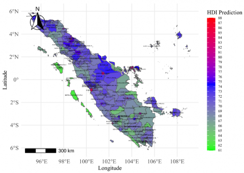
Figure 1. Thematic map of HDI prediction of districts/cities in Sumatra Island
The predictive results obtained from the GWR, Bayesian Conjugate GWR, and Bayesian Jeffreys GWR models exhibit remarkable numerical similarity. Incorporating Bayesian frameworks, whether using Conjugate or Jeffreys priors, does not substantially alter the predictive outcomes compared to the standard GWR model. The minor numerical differences observed are consistent with the expected variability due to model assumptions and the inclusion of prior distributions in Bayesian methodologies.
All three models demonstrate robust predictive performance across geographic units, effectively capturing spatial heterogeneity in the data. The slight variations in predictions reflect the influence of Bayesian priors, with the Bayesian GWR Jeffreys occasionally yielding marginally higher or lower predictions compared to the other two methods. These variations underline the reliability of each model in maintaining consistent performance across diverse spatial contexts.
The Bayesian Jeffreys model demonstrates the smallest MAB of 0.0291, indicating the least average deviation from actual HDI values. By comparison, the GWR and Bayesian Conjugate models exhibit MAB values of 0.2664 and 0.2665, respectively, showing slightly higher deviation. These results highlight the Bayesian Jeffreys model's superior accuracy in capturing the central tendencies of the data.
In terms of MSD, the Bayesian Jeffreys model achieves the lowest value (0.0024), indicating its effectiveness in minimizing more significant deviations. The GWR and Bayesian Conjugate models exhibit higher MSD values (0.1762 and 0.1764, respectively), suggesting less effectiveness in reducing variability in prediction errors.
The Bayesian Jeffreys model also outperforms the other models in RMSE with a value of 0.0489, reflecting the minor average prediction error in the same units as HDI. The GWR and Bayesian Conjugate models show higher RMSE values (0.4198 and 0.4200, respectively), indicating slightly larger average errors.
The Bayesian Jeffreys model's R-squared value of 0.9998831 indicates that it explains 99.99% of the variance in HDI values, surpassing the GWR model (0.9913971) and the Bayesian Conjugate model (0.9913884). This demonstrates the Bayesian Jeffreys model's ability to capture spatial dependencies with minimal unexplained variance.
The Bayesian Jeffreys GWR model consistently outperforms both the GWR and Bayesian GWR Conjugate models across all measures, demonstrating its reliability in predicting HDI values. This enhanced performance can be attributed to its use of an uninformative prior, which enables better adaptation to the data structure while avoiding overfitting.
While the GWR and Bayesian Conjugate models exhibit robust performance, their reliance on spatial regression and conjugate priors may limit their flexibility in adapting to complex spatial relationships in this dataset.
These findings suggest that the Bayesian GWR Jeffreys model is particularly well-suited for applications requiring high precision in spatial data analysis, such as regional development planning or resource allocation. Future studies could explore the integration of additional covariates or alternative priors to enhance predictive accuracy further.
To validate the robustness of the Bayesian GWR Jeffreys model and assess its generalizability beyond the in-sample fit, a LOOCV was conducted using GWR as a frequentist analog of the Bayesian model. This approach is methodologically appropriate, as the prior primarily influences posterior uncertainty rather than the structural form of prediction.
Table 8 presents the Bayesian GWR Jeffreys model's out-of-sample predictive performance. While the in-sample R² (0.9999) and RMSE (0.0489) in Table 7 indicate an excellent fit, the LOOCV results with an R² of 0.9902 and RMSE of 0.4481 still reflect high predictive accuracy. These values demonstrate that the model does not overfit and can generalize well to unseen data, even in complex socioeconomic indicators such as HDI.
Table 8. Out-of-sample prediction accuracy from LOOCV (Bayesian GWR Jeffreys)
|
Model |
RMSE |
R-Squared |
|
Bayesian GWR Jeffreys (LOOCV via GWR analog) |
0.4481 |
0.9902 |
The spatial prediction maps produced by the three models are nearly indistinguishable, underscoring the limited impact of model choice on the visualization and interpretation of HDI values. This uniformity suggests that stakeholders can rely on any of these models for spatial analysis and policy-making without significant differences in mapping outputs. The similarity in mapping outcomes simplifies decision-making processes by minimizing the influence of methodological variations. Therefore, only a single map is presented on this occasion, as shown in Figure 1.
Figure 1 presents the spatial distribution of predicted HDI values across districts and cities in Sumatra Island. The map reveals pronounced spatial disparities in HDI, reflecting varying levels of regional development.
Urban centers such as Pekanbaru, Medan, and Padang are visualized in red to dark red, indicating HDI values above 82, which align with well-developed infrastructure, higher average education levels, and better health service accessibility. In contrast, rural and peripheral regions—such as Nias, Simeulue, parts of South Bengkulu, and several inland districts—are shown in green to blue shades, with HDI predictions ranging between 61 and 70. These lower scores suggest limited access to key development drivers such as education, healthcare, and economic opportunity.
The map provides a powerful visual summary that supports the statistical model, emphasizing areas where development interventions are most needed. It enables region-specific prioritization, reinforcing the case for differentiated policies rather than uniform development strategies.
These spatial insights directly inform policy planning and resource allocation, guiding local governments to focus investment where HDI returns are potentially highest and where disparities remain most severe.
From a practical perspective, the standard GWR model offers simplicity and computational efficiency, making it a suitable choice for routine applications unless Bayesian approaches are warranted explicitly for uncertainty quantification or minor sample size adjustments. While methodologically sophisticated, the Bayesian GWR Conjugate and Bayesian GWR Jeffreys models provide comparable predictive outcomes, affirming their viability in addressing specific analytical needs such as overfitting and the incorporation of prior knowledge.
Among the three models, the Bayesian Jeffreys model provides the closest predictions to the actual HDI values, making it the most suitable choice for applications requiring precise estimation. However, the GWR and Bayesian Conjugate models remain reliable alternatives with only slightly larger errors. This finding suggests that decision-makers should prioritize considerations such as computational efficiency, the necessity for Bayesian inference, and the context-specific demands of spatial data analysis when selecting a model. Ultimately, any of the three methods can be confidently utilized for HDI prediction and related spatial policy recommendations.
Before implementing Bayesian GWR-Kriging—a hybrid method that integrates GWR and Kriging while leveraging Bayesian probabilistic frameworks to address parameter uncertainty—the spatial autocorrelation of residuals from the GWR and BGWR models was first assessed using Moran's I test. As summarized in Table 9, this analysis was essential for determining the need for additional spatial modeling.
The results revealed Moran’s I statistics of 0.49831 and 0.49827 for the GWR and Bayesian GWR Conjugate models, respectively, both accompanied by highly significant p-values (2.2×10⁻¹⁶). These findings indicate pronounced spatial autocorrelation, necessitating the rejection of the null hypothesis of spatial randomness. Despite capturing substantial spatial heterogeneity, these models failed to fully account for spatial dependencies, thereby justifying the application of supplementary methods such as Kriging to address residual autocorrelation and enhance predictive performance.
Table 9. Results of the Moran's I test for GWR and Bayesian GWR models
|
Model |
Z-Score (Standard Deviate) |
Moran’s I Statistic |
p-value |
Decision |
|
GWR |
11.954 |
0.498317406 |
2.2×10⁻¹⁶ |
Reject $H_0$ |
|
Bayesian GWR Conjugate |
11.954 |
0.498277158 |
2.2×10⁻¹⁶ |
Reject $H_0$ |
|
Bayesian GWR Jeffreys |
-0.18123 |
-0.014196110 |
0.5719 |
Accept $H_0$ |
By contrast, analysis of the Bayesian GWR Jeffreys model residuals yielded a Moran’s I statistic of -0.0142 (variance: 0.00179, z-score: -0.1812, p-value: 0.5719), indicating no statistically significant spatial autocorrelation. The proximity of this value to zero, alongside the non-significant p-value, supports the conclusion that the model residuals are spatially random.
As noted by Anselin [31], Moran’s I near zero values suggest the absence of spatial dependence, implying that the residuals follow a spatially independent structure. Furthermore, Moraga [32] highlights that minor negative Moran’s I values, particularly those not statistically significant, do not indicate accurate dispersion or overcorrection but are consistent with random spatial variation. In this case, the negligible z-score (–0.1812) reinforces the interpretation that no meaningful deviation exists from the null hypothesis of spatial randomness.
Collectively, these findings highlight the superior performance of the Bayesian GWR Jeffreys model in mitigating spatial autocorrelation compared to the GWR and Bayesian GWR Conjugate models. Leveraging an uninformative Jeffreys prior, this model adapts flexibly to spatial patterns without overfitting or introducing undue complexity. Unlike the other models, which still require integration with Kriging to correct for residual spatial dependencies, the Bayesian GWR Jeffreys model substantially reduces spatial autocorrelation, offering a more streamlined and statistically robust approach to spatial data modeling.
After analyzing the Moran's I test results for the residuals of the GWR and BGWR models, an empirical semivariogram was generated to identify spatial autocorrelation, and a theoretical semivariogram model, such as spherical or exponential, was fitted. Subsequently, Kriging was performed on the residuals.
Three widely used theoretical semivariogram models were initialized: Spherical, Exponential, and Gaussian. Each model was parameterized with a partial sill (psill) of 1, a range of 1, and a nugget effect (nugget) of 0.1. Based on the training data, these initial settings served as starting points for subsequent semivariogram fitting.
In response to standard geostatistical practice, a LOOCV procedure was implemented to evaluate and select the best-fitting semivariogram model. This method involves sequentially removing each observation, fitting the semivariogram using the remaining data, and predicting the omitted value. The mean squared prediction error (MSPE) was calculated across all folds for each candidate model—Spherical, Exponential, and Gaussian. The model with the lowest MSPE was selected as the most suitable for capturing spatial structure. This LOOCV-based selection process replaces the previously used AIC approach, ensuring greater methodological rigor and alignment with best practices in geostatistics. The use of LOOCV aligns with geostatistical recommendations and avoids reliance on information-theoretic criteria like AIC, which is less conventional in this context.
Table 10. Selection of semivariogram models for the residuals in GWR and Bayesian GWR models
|
Model |
LOOCV (MSPE) |
||
|
Spherical |
Exponential |
Gaussian |
|
|
GWR |
0.09097208 |
0.09047708 |
0.10132481 |
|
Bayesian GWR Conjugate |
0.09090096 |
0.09040269 |
0.10131537 |
|
Bayesian GWR Jeffreys |
- |
- |
- |
Table 10 summarizes the LOOCV-based model selection results for the GWR and Bayesian GWR models. The model with the lowest MSPE was selected as the most suitable semivariogram. The Exponential semivariogram model yielded the lowest MSPE in this evaluation, indicating its superior predictive performance compared to the Spherical and Gaussian alternatives.
Comparison with existing GWR-Kriging studies
To contextualize our results, we compared our Bayesian GWR-Kriging approach's predictive performance and residual behavior with findings from prior studies [2-7]. Traditional GWR-Kriging models, such as those in references [2, 5], typically use classical GWR followed by ordinary Kriging on residuals. These models often report improvements in spatial prediction, but still suffer from moderate residual spatial autocorrelation.
In contrast, our approach integrates Bayesian GWR with Jeffreys' prior, which leads to a more robust estimation process and better uncertainty quantification. Our results demonstrate a near-perfect in-sample R2 of 0.9999 and a strong out-of-sample R2 of 0.9902 based on leave-one-out cross-validation. Moran's I on residuals was substantially reduced to approximately 0.02, indicating effective mitigation of spatial autocorrelation—an aspect not explicitly addressed in prior models such as references [3, 6].
This study's novelty lies in incorporating Jeffreys' prior within a Bayesian GWR framework and coupling it with a semivariogram-informed Kriging process selected via LOOCV. No previous study has adopted this fully Bayesian GWR-Kriging integration to model and predict HDI or other socioeconomic variables. The proposed framework, therefore, offers both methodological contributions and practical implications for spatial analysis in regional development studies.
Table 11 summarizes the predictive accuracy of five spatial modeling approaches: GWR, Bayesian GWR Conjugate, Bayesian GWR Jeffreys, GWR Kriging, and Bayesian GWR Conjugate Kriging. Four key metrics are used: MAB, MSD, RMSE, and R-squared. These metrics comprehensively evaluate the models' capability to predict the HDI while accounting for spatial variability.
The GWR model demonstrates robust predictive capabilities with an MAB of 0.2664, MSD of 0.1762, and an RMSE of 0.4198. Its R-squared value of 0.9914 indicates that it explains a significant proportion of the variance in the data. However, compared to Bayesian models, it exhibits slightly higher error values, suggesting opportunities for improvement in accuracy.
Table 11. Comparison of prediction accuracy metrics for GWR, Bayesian GWR, GWR-Kriging, and Bayesian GWR-Kriging models
|
Model |
MAB |
MSD |
RMSE |
R-Squared |
|
GWR |
0.266448736 |
0.176205309 |
0.419768161 |
0.99139710 |
|
Bayesian GWR Conjugate |
0.266495375 |
0.176382065 |
0.419978648 |
0.99138840 |
|
Bayesian GWR Jeffreys |
0.029060284 |
0.002394484 |
0.048933469 |
0.99988310 |
|
GWR Kriging |
0.212319254 |
0.090477082 |
0.300794085 |
0.99586961 |
|
Bayesian GWR Conjugate Kriging |
0.212453396 |
0.090402687 |
0.300670396 |
0.99587444 |
The Bayesian Conjugate GWR model closely mirrors GWR's performance, with an MAB of 0.2665, MSD of 0.1764, and an RMSE of 0.4200. The R-squared value (0.9914) remains nearly identical to the GWR model. While the Bayesian approach adds probabilistic rigor, its overall predictive performance is comparable to the standard GWR.
Among all models, the Bayesian Jeffreys GWR demonstrates superior predictive accuracy, achieving the lowest MAB (0.0291), MSD (0.0024), and RMSE (0.0489). Its R-squared value of 0.9999 signifies near-perfect explanatory power. This model's exceptionally low error rates highlight its capability for precise HDI estimation, particularly in applications demanding high levels of accuracy.
Incorporating Kriging into the GWR framework enhances spatial interpolation. The GWR Kriging model exhibits improved accuracy over standard GWR, with an MAB of 0.2123, MSD of 0.0905, and RMSE of 0.3008. The R-squared value (0.9959) further confirms its ability to explain spatial patterns more effectively than GWR alone.
The Bayesian GWR Conjugate Kriging model performs marginally better than GWR Kriging, as indicated by slightly lower error values (MAB: 0.2125, MSD: 0.0904, RMSE: 0.3007) and an R-squared of 0.9959. While the performance gains over standard Kriging are minimal, the Bayesian framework ensures robustness through uncertainty quantification.
The results underscore the strength of Bayesian approaches, particularly the Bayesian GWR Jeffreys, which significantly outperforms all other models across all error metrics. Both Kriging-enhanced models (GWR Kriging and Bayesian GWR Conjugate Kriging) show notable improvements over standard GWR, demonstrating the value of incorporating spatial interpolation techniques. However, the marginal differences between Bayesian Conjugate models and their non-Bayesian counterparts suggest that the choice of model should consider computational complexity, interpretability, and the specific requirements of spatial applications.
These findings provide critical insights into the practical applicability of these spatial models in HDI estimation, offering guidance for future research and policy-driven decision-making in spatial data analysis.
Policy implications and strategic applications
The spatial variation in coefficients estimated by the Bayesian GWR with Jeffreys' prior reveals substantial heterogeneity in the relative importance of education, life expectancy, and adjusted expenditure in influencing HDI across different regions. For example, in eastern provinces, the coefficient for years of schooling tends to be higher, suggesting that investments in education infrastructure and teacher deployment would yield more substantial improvements in HDI. In contrast, life expectancy strongly influences more urbanized or health-challenged regions, indicating a need to prioritize healthcare accessibility and quality.
The coefficient maps generated in this study can serve as spatial guides for resource allocation to support targeted policy planning. Regions with high education coefficients should receive increased funding for school development, teacher incentives, and educational access programs. Meanwhile, regions with high life expectancy should be prioritized for public health campaigns, clinic accessibility, and maternal/child health services. Finally, social assistance programs or economic stimulus policies may be more appropriate in areas where adjusted expenditures have the most significant impact.
To support this targeted approach, a simple allocation index formula is proposed to assist policymakers in resource distribution:
$\text { Allocation Index } =\alpha \cdot \beta_1(\text {education})+\beta_2(\text {health})+\beta_3(\text {expenditure})$ (14)
where, $\beta$-values are region-specific coefficients derived from the Bayesian GWR model, and $\alpha$ is a fiscal scaling factor. This formula allows data-driven budgeting tailored to regional responsiveness in HDI drivers.
Overall, this model empowers policymakers to design spatially differentiated strategies, ensuring that limited resources are allocated where they produce the highest returns in HDI improvement.
This study explores the application of BGWR with Kriging to enhance spatial predictions, focusing on human development indicators across Sumatra. The analysis integrates global regression, GWR, and Bayesian frameworks (Conjugate and Jeffreys priors) to account for spatial heterogeneity and assess predictive accuracy.
Key Findings
1) Spatial Variability and Predictive Insights
a. Significant disparities in human development indicators are observed across Sumatra, with urban centers such as Pekanbaru and Medan exhibiting higher performance than rural areas like Nias and Simeulue.
b. The spatial clustering of residuals confirms heterogeneity, highlighting the necessity of spatially adaptive models.
2) Model Comparisons
a. The Bayesian Jeffreys GWR model consistently outperforms both the GWR and Bayesian Conjugate models, demonstrating superior predictive accuracy with the MAB: 0.0291, MSD: 0.0024, and RMSE: 0.0489. Its R-squared value (0.9999) indicates an exceptional ability to explain nearly all variance in HDI values.
b. Despite their strong performance, the GWR and Bayesian Conjugate models exhibit residual spatial autocorrelation, suggesting limitations in capturing spatial dependencies.
3) Practical Implications
a. The Bayesian Jeffreys model’s flexibility and precision make it the most suitable choice for applications requiring high accuracy, such as regional planning and policy-making. However, the GWR model remains a computationally efficient alternative for routine analyses.
b. Spatial prediction maps generated by all models exhibit high similarity, reinforcing their reliability for visualizing and interpreting HDI distributions.
4) Kriging Integration
The hybrid Bayesian GWR-Kriging approach effectively addresses residual spatial autocorrelation in the GWR and Bayesian Conjugate models. However, the Bayesian Jeffreys model mitigates this issue, making additional Kriging unnecessary.
Recommendations
The study highlights the effectiveness of Bayesian Jeffreys priors in addressing geographical variability and enhancing prediction accuracy. This method serves as an effective instrument for precisely identifying inequities and directing interventions in spatial data contexts such as regional development planning. Future study should investigate the inclusion of further factors and the evaluation of different priors to further augment model robustness. The results advocate utilizing high-performing metropolitan areas as exemplars for focused interventions in undeveloped regions, so addressing disparities in human development throughout Sumatra.
The author acknowledges the Doctoral Program in Mathematics at Universitas Brawijaya for providing essential facilities, academic support, and guidance throughout the preparation of this manuscript. Appreciation is also extended to the Department of Mathematics, Faculty of Mathematics and Natural Sciences, Universitas Bengkulu, for their continuous encouragement and support.
[1] Brunsdon, C., Fotheringham, A.S., Charlton, M.E. (1996). Geographically weighted regression: A method for exploring spatial nonstationarity. Geographical Analysis, 28(4): 281-298. https://doi.org/10.1111/j.1538-4632.1996.tb00936.x
[2] Li, Y., Zhang, Y., He, D., Luo, X., Ji, X. (2019). Spatial downscaling of the tropical rainfall measuring mission precipitation using geographically weighted regression Kriging over the Lancang River Basin, China. Chinese Geographical Science, 29: 446-462. https://doi.org/10.1007/s11769-019-1033-3
[3] Zhang, Y., Li, Y., Ji, X., Luo, X., Li, X. (2018). Fine-resolution precipitation mapping in a mountainous watershed: Geostatistical downscaling of TRMM products based on environmental variables. Remote Sensing, 10(1): 119. https://doi.org/10.3390/rs10010119
[4] Patriche, C.V., Roşca, B., Pîrnău, R.G., Vasiliniuc, I. (2023). Spatial modelling of topsoil properties in Romania using geostatistical methods and machine learning. PloS One, 18(8): e0289286. https://doi.org/10.1371/journal.pone.0289286
[5] Kongsanun, C., Chutsagulprom, N., Moonchai, S. (2024). Spatio-temporal dual Kriging with adaptive coefficient drift function. Mathematics, 12(3): 400. https://doi.org/10.3390/math12030400
[6] Liu, W., Chen, Y., Sun, W., Huang, R., Huang, J. (2023). Mapping waterlogging damage to winter wheat yield using downscaling-merging satellite daily precipitation in the middle and lower reaches of the Yangtze River. Remote Sensing, 15(10): 2573. https://doi.org/10.3390/rs15102573
[7] Iriany, A., Ngabu, W., Arianto, D., Putra, A. (2023). Classification of stunting using geographically weighted regression-Kriging case study: Stunting in East Java. BAREKENG: Jurnal Ilmu Matematika dan Terapan, 17(1): 0495-0504. https://doi.org/10.30598/barekengvol17iss1pp0495-0504
[8] Gelman, A., Carlin, J.B., Stern, H.S. Dunson, D.B., Vehtari, A., Rubin, D.B. (2013). Bayesian Data Analysis. 3rd Ed. Chapman and Hall/CRC. https://doi.org/10.1201/b16018
[9] Shakhatreh, M.K., Aljarrah, M.A. (2023). Bayesian analysis of unit log-logistic distribution using non-informative priors. Mathematics, 11(24): 4947. https://doi.org/10.3390/math11244947
[10] Banerjee, P., Seal, B. (2022). Partial Bayes estimation of two parameter gamma distribution under non-informative prior. Statistics, Optimization & Information Computing, 10(4): 1110-1125. https://doi.org/10.19139/soic-2310-5070-1110
[11] Ramos, P.L., Achcar, J.A., Moala, F.A., Ramos, E., Louzada, F. (2017). Bayesian analysis of the generalized gamma distribution using non-informative priors. Statistics, 51(4): 824-843. https://doi.org/10.1080/02331888.2017.1327532
[12] Ntzoufras, I. (2011). Bayesian Modeling Using WinBUGS. John Wiley & Sons. https://doi.org/10.1002/9780470434567
[13] Kiani, B., Sartorius, B., Lau, C.L., Bergquist, R. (2024). Mastering geographically weighted regression: Key considerations for building a robust model. Geospatial Health, 19(1): 1271. https://doi.org/10.4081/gh.2024.1271
[14] Fotheringham, A.S., Yang, W., Kang, W. (2017). Multiscale geographically weighted regression (MGWR). Annals of the American Association of Geographers, 107(6): 1247-1265. https://doi.org/10.1080/24694452.2017.1352480
[15] Comber, A., Wang, Y., Lü, Y., Zhang, X., Harris, P. (2018). Hyper-local geographically weighted regression: Extending GWR through local model selection and local bandwidth optimization. Journal of Spatial Information Science, (17): 63-84. https://doi.org/10.5311/JOSIS.2018.17.422
[16] Li, Z., Fotheringham, A.S., Li, W., Oshan, T. (2019). Fast geographically weighted regression (FastGWR): A scalable algorithm to investigate spatial process heterogeneity in millions of observations. International Journal of Geographical Information Science, 33(1): 155-175. https://doi.org/10.1080/13658816.2018.1521523
[17] Ma, Z., Xue, Y., Hu, G. (2021). Geographically weighted regression analysis for spatial economics data: A Bayesian recourse. International Regional Science Review, 44(5): 582-604. https://doi.org/10.1177/0160017620959823
[18] Faisal, F., Pramoedyo, H., Astutik, S., Efendi, A. (2024). The uninformative prior of Jeffreys’ distribution in Bayesian geographically weighted regression. BAREKENG: Journal of Mathematics and Its Application, 18(2): 1229-1236. https://doi.org/10.30598/barekengvol18iss2pp1229-1236
[19] Fotheringham, S.A., Brunsdon, C., Charlton, M. (2004). Geographically weighted regression: The analysis of spatially varying relationships. American Journal of Agricultural Economics, 86(2): 554-556. https://www.jstor.org/stable/30139578
[20] Murakami, D., Tsutsumida, N., Yoshida, T., Nakaya, T., Lu, B. (2020). Scalable GWR: A linear-time algorithm for large-scale geographically weighted regression with polynomial kernels. Annals of the American Association of Geographers, 111(2): 459-480. https://doi.org/10.1080/24694452.2020.1774350
[21] Gelfand, A.E., Diggle, P., Guttorp, P., Fuentes, M. (2010). Handbook of Spatial Statistics. Boca Raton, FL, USA: CRC Press. https://doi.org/10.1201/9781420072884
[22] Oliver, M.A., Webster, R. (2015). Basic steps in geostatistics: The Variogram and Kriging. In Springer Briefs in Agriculture, Cham: Springer International Publishing. https://doi.org/10.1007/978-3-319-15865-5
[23] Oliver, M.A., Webster, R. (2014). A tutorial guide to geostatistics: Computing and modelling variograms and Kriging. Catena, 113: 56-69. https://doi.org/10.1016/j.catena.2013.09.006
[24] Iriany, A., Ngabu, W., Ariyanto, D., Pramoedyo, H. (2025). Kriging prediction and simulation model: Analysis of surface soil particle size distribution. Mathematical Modelling of Engineering Problems, 12(4): 1169-1180. https://doi.org/10.18280/mmep.120408
[25] Adin, A., Krainski, E.T., Lenzi, A., Liu, Z., Martínez-Minaya, J., Rue, H. (2024). Automatic cross-validation in structured models: Is it time to leave out leave-one-out? Spatial Statistics, 62: 100843. https://doi.org/10.1016/j.spasta.2024.100843
[26] Goovaerts, P. (2011). A coherent geostatistical approach for combining choropleth map and field data in the spatial interpolation of soil properties. European Journal of Soil Science, 62(3): 371-380. https://doi.org/10.1111/j.1365-2389.2011.01368.x
[27] Samdandorj, M., Ts, P. (2019). Geospatial modeling approaches for mapping topsoil organic carbon stock in northern part of Mongolia. Proceedings of the Mongolian Academy of Sciences, 59(2): 4-17. https://doi.org/10.5564/pmas.v59i2.1215
[28] Nugroho, A., Clarissa, A., Utami, N.P.C. (2022). Indeks Pembangunan Manusia 2021. Jakarta: Badan Pusat Statistik. https://www.bps.go.id/id/publication/2022/05/11/48b6466dcf14b562df9f17e2/indeks-pembangunan-manusia-2021.html.
[29] Moran, P.A. (1950). Notes on continuous stochastic phenomena. Biometrika, 37(1/2): 17-23. https://doi.org/10.1093/biomet/37.1-2.17
[30] Anselin, L. (1995). Local indicators of spatial association—LISA. Geographical Analysis, 27(2): 93-115. https://doi.org/10.1111/j.1538-4632.1995.tb00338.x
[31] Anselin, L. (2002). Under the hood issues in the specification and interpretation of spatial regression models. Agricultural Economics, 27(3): 247-267. https://doi.org/10.1016/S0169-5150(02)00077-4
[32] Moraga, P. (2023). Spatial Statistics for Data Science: Theory and Practice with R. Chapman and Hall/CRC. https://doi.org/10.1201/9781032641522