Muataz I. Ali*![]() | Hiba A. Abu-Alsaad
| Hiba A. Abu-Alsaad![]()
© 2025 The authors. This article is published by IIETA and is licensed under the CC BY 4.0 license (http://creativecommons.org/licenses/by/4.0/).
OPEN ACCESS
The objective of this research paper is to utilise artificial neural networks (ANNs) in order to propose an analytical method for establishing constitutive correlations for normal-strength concrete (NSC) and high-strength concrete (HSC) in fire situations. The goal is to create a useful model and outline the fire-performance specifications for concrete structures in fire situations. The outcomes of NSC and high-strength concrete (HSC) were evaluated using reactive error distribution techniques and multiple layered networks. The multi-layered networks with reactive error distribution technology assign weights to each variable, which impacts the strength of concrete. Elevated temperatures have a detrimental effect on both NSC and HSC. With a correlation coefficient of 96.2%, a determination coefficient of 92.7%, a mean absolute percentage error (MAPE) of 7.3%, and a determination coefficient (R2) of 89.6%, the ANNs were able to accurately predict the compressive strength of concrete at high temperatures.
ANN, constitutive models, fire, high-strength concrete HSC, normal-strength concrete NSC, elevated temperatures, estimate model
The fire safety designing of high-rise buildings and infrastructures involves providing various measures that must be included in any design for it to be considered safe. In these circumstances, concrete is one of the main materials that may be considered in its structural design. At the moment, reinforced concrete (RC) members' fire resistance can be provided through prescriptive approaches involving either the use of standard fire-resistance tests or empirical calculation methods [1-6]. Despite the limitations of extensively benefiting from either of these approaches, there are no heavily publicised failing structures or structural components made of normal-strength concrete (NSC) and high-strength concrete (HSC) if they are well-designed after the relevant rules in the loading and fire analysis. Recently, there has been a growing interest in utilising numerical approaches to assess the fire resistance of structural elements. It is well known that concrete behaviours at temperatures, such as during a fire, vary with concrete materials constituents [7].
At normal temperatures, there are several compressive constitutive models for concrete. However, it’s very difficult to comprehend how concrete material behaves at high temperatures, as current knowledge of the material's thermal characteristics at high temperatures is based on a small number of experimental test investigations. The test data of some high temperature properties of concrete are very scarce and the test data of other properties of concrete at high temperatures are significantly different and inconsistent [8-10]. These inconsistencies and discrepancies are primarily attributed to the variations in test methodologies and procedural settings as well as environmental conditions during testing [4].
The fire resistance in building codes for the protection of structural members is almost exclusively (but not exclusively) based on the properties of the materials that the structural members are made of, with little regard to the geometry of the structural members [11]. Therefore, to be competent in evaluating concrete mixtures in light of performance-based building codes, a competent understanding of the high-temperature characteristics of concrete is necessary [12]. Some interaction occurs between the cement paste drying and aggregates’ thermal expansion. It seems that limestone aggregates, which have a lower thermal coefficient of expansion than siliceous aggregates, may help produce concretes that resist disintegration due to such a cause at high temperatures [13].
High-strength concrete (HSC), with compressive strength above a similar limit of NSC, which is 55.2 MPa, was demonstrated that they are not the same under high temperatures according to early investigations [14, 15]. Degradation of HSC is faster, according to Diederichs, Kodur and Phan [3, 15, 16]. Therefore, the present high-temperature relationships, primarily based on limited fire testing of the traditional NSC material, must be carefully evaluated before being applied to HSC [10].
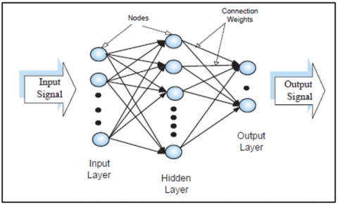
Artificial neural networks (ANNs) are computational models which mimic the construction and primitive operation of biological neural networks. It can be used to solve nonlinear problems or have excess data, which they can solve very quickly [17, 18]. Many researchers have shown that neural networks are a powerful tool for practical classification tasks and solving all kinds of intricate structural and civil engineering problems where there are limited or it does not exist an adequate or sufficient amount of data [19, 20]. All ANNs have an identical structure or topology, which involves arranging neurons in a succession of layers, as depicted in Figure 1.
Figure 1. Architecture of the neural network
In ANN, the first layer takes in raw data, either from sensors or input files, and processes it as independent variables or features. The final layer produces the predicted values or classes, which can then be sent to external systems like mechanical controllers or other computer programs [21]. The middle layers, also known as hidden layers, consist of several neurons with varying connection topologies. The model features NNN inputs and a single output. The neuron’s soma contains a summing junction (Σ) and an activation function f(x), both of which are characteristic features of artificial neurons [22].
The weight assigned to each input determines its contribution to the summation function. The output activation is influenced by the node’s internal bias (b), which remains constant. The input vector consists of elements (x1, x2, ..., xN), while the weight vector consists of elements (w1, w2, ..., wN). The summing function is obtained by multiplying vector x (input vector) and vector w (weight vector), followed by adding the resulting products, as shown in Eq. (1):
$a=\sum_{i=1}^N\left(w_i x_i\right)+b$ (1)
The output is a single value. A transfer function technique is then used to process this weighted total, yielding the final result for analysis. If the neuron generates a strong enough signal, the output is 1; otherwise, it is 0. Various types of transfer functions exist to match different models with the range of outputs a neuron can produce [23, 24].
This study aims to develop a model to establish relationships between elevated temperatures and compressive strength, specifically focusing on the residual compressive strength of NSC and HSC. The model will use ANNs to derive an arithmetic formula that can be employed by researchers for predicting the fire resistance of reinforced concrete (RC) members, where the proposed model has two inputs (fc and T). In contrast, previous models were based on one variable (T) and this variable, through data analysis in the current research, proved that there is a change in (fc) with (T) whenever the amount of (fc) changes by ten units (10 MPa).
The investigation of NSC residual compressive behaviour continued during the early 1960s by many researchers [3, 16, 25]. Since compressive strength is the strength of a material that has been heated in a product and then cooled to a specific test temperature content at room temperature, emphasis has resulted from this research. Residual strains, along with strength recovery with time, are included in the analysis. Table 1 summarises important versions that regarded the eased strength of concrete by fire in the literature. Another connection suggested for examination is the compressive strength of NSC and HSC with siliceous aggregate. In regression analysis, the primary goals are to inspect the changing experimental compressive strength of NSC behaviours in elevated temperatures and to offer clear and simple correlations that systematically correlate nicely with experimental data.
The relationship between the uniaxial compressive strength of NSC at various temperatures is determined by unstressed experimental experiments. In these tests, a specimen is heated without any pre-loading, and the temperature is increased at a steady pace. Several researchers have conducted studies on the impact of temperature on NSC using direct visual observation. Normally, the compressive strength of NSC decreases by approximately 10-20% when it is heated to 300℃ [2-4, 6, 29]. The temperature at which the maximum rate of decay for cement uniaxial compression first develops of strength is about 60-75% for heating to 600℃. Extreme values for NSC strength at elevated are obtained from the Lie et al. [26, 27].
Table 1. Compressive strength models of concrete at high temperatures
|
References |
Compressive Strength at Elevated Temperatures |
|
Lie et al. [27] |
$f_{c T}^{\prime}=f_c^{\prime}\left(2.011-2.353 \frac{T-20}{1000}\right) \leq f_c^{\prime}$ |
|
Eurocode 2 [28] |
$f_{c T}^{\prime}=f_c^{\prime}(1-0.001 T) T \leq 500^{\circ} \mathrm{C}$, $f_{c T}^{\prime}=f_c^{\prime}(1.375-0.00175 T) 500^{\circ} \leq T \leq 700^{\circ} \mathrm{C}$, $f_{c T}^{\prime}=0 \quad T \geq 700^{\circ} \mathrm{C}$ |
|
ASCE [29] |
$f_{c T}^{\prime}=f_c^{\prime} \quad T \leq 100^{\circ} \mathrm{C}$, $f_{c T}^{\prime}=f_c^{\prime}(1.067-0.00067 T) \quad 100^{\circ} \mathrm{C} \leq T \leq 400^{\circ} \mathrm{C}$, $f_{c T}^{\prime}=f_c^{\prime}(1.44-0.0016 T) \quad T \geq 400^{\circ} \mathrm{C}$ |
|
Lie and Erwin [30] |
$f_{c T}^{\prime}=f_c^{\prime} \quad 20^{\circ} \leq T \leq 450^{\circ} \mathrm{C}$, $f_{c T}^{\prime}=f_c^{\prime}\left[2.011-2.353\left(\frac{T-20}{1000}\right)\right] \quad 450^{\circ} \leq T \leq 874^{\circ} \mathrm{C}$, $f_{c T}^{\prime}=0 \quad T>874^{\circ} \mathrm{C}$ |
|
Chang and Jau [31] |
$f_{c T}^{\prime}=f_c^{\prime} \quad 0^{\circ} \mathrm{C} \leq T<450^{\circ} \mathrm{C}$, $f_{c T}^{\prime}=f_c^{\prime}\left(2.06-\left(\frac{T}{425}\right)\right) \quad T \geq 450^{\circ} \mathrm{C}$ |
|
Kodur et al. [32] |
$f_{c T}^{\prime}=(1-0.001 T) f_c^{\prime} \quad 0^{\circ} \mathrm{C} \leq T \leq 500^{\circ} \mathrm{C}$, $f_{c T}^{\prime}=\left[1.6046+\left(1.3 T^2-2817 T\right) \times 10^{-6}\right] f_c^{\prime} \quad T>500^{\circ} \mathrm{C}$ |
|
Li and Purkiss [33] |
$f_{c T}^{\prime}=\left\{\begin{array}{cc}f_c^{\prime}[1.0-0.003125(T-20)] & T<100^{\circ} \mathrm{C} \\ 0.75 f_c^{\prime} & 100^{\circ} \mathrm{C} \leq T \leq 400^{\circ} \mathrm{C} \\ f_c^{\prime}[1.33-0.00145 T] & 400^{\circ} \mathrm{C}<T\end{array}\right\}$ |
|
Chang et al. [34] |
$f_{c T}^{\prime}=f_c^{\prime}\left(0.00165\left(\frac{T}{100}\right)^3-0.03\left(\frac{T}{100}\right)^2+0.025\left(\frac{T}{100}\right)+1.002\right)$ |
|
Bastami and Aslani et al. [35] |
$f_{c T}^{\prime}=f_c^{\prime}\left(1.008+\frac{T}{450 \ln \left(\frac{T}{5800}\right)}\right) \geq 0.0 \quad 20^{\circ} \mathrm{C}<T \leq 800^{\circ} \mathrm{C}$, $f_{c T}^{\prime}=f_c^{\prime}\left\{\begin{array}{ll}1.01-0.00055 T & 20^{\circ} \mathrm{C}<T \leq 200^{\circ} \mathrm{C} \\ 1.15-0.00125 T & 200^{\circ} \mathrm{C} \leq T \leq 800^{\circ} \mathrm{C}\end{array}\right\}$ |
|
Lie et al. [27] |
$f_{c T}^{\prime}=f_c^{\prime}\left[\begin{array}{cc}1.012-0.0005 T \leq 1.0 & 20^{\circ} \mathrm{C} \leq T \leq 100^{\circ} \mathrm{C} \\ 0.985+0.0002 T-2.235 \times 10^{-6} T^2+8 \times 10^{-10} T^3 & 100^{\circ} \mathrm{C}<T \leq 800^{\circ} \mathrm{C} \\ 0.44-0.0004 \mathrm{~T} & 900^{\circ} \mathrm{C} \leq T \leq 1000^{\circ} \mathrm{C} \\ 0 & T>1000^{\circ} \mathrm{C}\end{array}\right]$ |
A relationship between high & ultra-HSC contains siliceous aggregate (55.2 to 80 MPa) and (80 to 110 MPa) of different aggregates; thermal was verified and reported in Table 1, and also listed the available published unstressed experimental results taken from various sources [2-6] which sets the valuable information for experiment, because Table 1 has many loading combinations of temperature and average concrete strength. Lie and Lin [26] defined a more tightly defined upper limit for concrete, showing an upper limit for fcT. Castillo [2] studied the compressive behaviour of concrete; he calculated the strength loss of HSC up to a temperature of 450℃, and the strength loss is higher up to about 40%. Also, the strength ratio between Singapore fly ash concrete and corresponding Portland cement concrete was as low as 0.6. If the test is conducted for another ratio of mixes, the results are directly related to the test’s compressive strength. the distinguishes the ANNs is that the expected result appears based on a single equation and is not divided into sections, in addition to the fact that the expected result in the neural network model depends on estimating the missing values based on the known values (deals with disconnected, unconnected data).
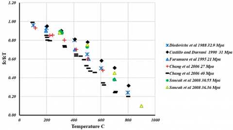
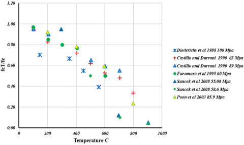
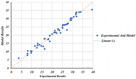
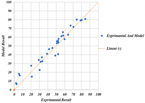
The data was collected based on the researchers’ previous experiments, which were used by previous researchers in comparing the previously proposed models [2-6, 29, 30] as in Figure 2. The previous models relied on the relationship between temperature and the residual ratios of the compressive strength (fc/fcT). In collecting data, both the compressive strength was taken before and after exposure to high temperature, in addition to temperature, since it was observed that the ratios of compressive strength reduction are dependent on the compressive strength and alter whenever the compressive strength varies by 10 MPa. Thus, the inputs in the proposed model will be two inputs and one output, in contrast to the rest of the models that take one input. and one output. The number of data collected from previous researches for the purpose of constructing and training the model of an ANNs to determine the compressive strength of the NSC was 132 collected from 8 previous researches, while for HSC constructing and training the model it was 89.
(a) NSC (20-40) MPa
(b) HSC (50-110) MPa
Figure 2. Data collection from previous researchers
An ANN was employed to analyze and forecast how NSC and HSC will interact structurally. The variables to be entered into the model were chosen by the ANN, enabling simulations that forecast the concrete's compressive strength at elevated temperatures.
There are feed-forward neural networks, self-regulated Cohon and Pyreptron [17, 22]. Back-propagation feed-forward, which comprised interconnected layers of neurons, was used in the work. Every individual neuron inside a given layer forms connections with every other neuron in the subsequent layer. Typically, these networks consist of three neural layers: input, hidden, and output. Figure 1 shows that the input layer does not undergo any processing. Exactly at the point where the network transmits radiation data. Data is transmitted from the input layer to the hidden layer. Next, the concealed layer transmits the output. The study uses an ANN made up of several sub-models, including input and output models, data division, neural network design selection, model weighting, and validation. The SPSS program was used to apply artificial intelligence techniques and create multiple neural networks. This approach helps demonstrate how the different components work together, from input to output.
The study uses an ANN with several sub-models, including input and output models, data division, neural network design selection, model weighting, and validation. The SPSS software was utilized as a tool for executing artificial intelligence methodologies and constructing diverse ANNs. This application was utilized to demonstrate the procedure of creating a sub-model from input to output model.
5.1 A statistical study using ANNs
5.1.1 Normal-strength concrete NSC
Two independent variables make up the input data in the input model: normal compressive strength (fc) and temperature (T). The output data is the compressive strength at elevated temperature (fcT). The data were partitioned into three distinct groups: a training group, which was used to optimise the weights associated with ANNs; a testing group, which was used to assess the network’s performance; and a validation group, it was employed to assess the overall performance of the model. Training was halted when the error rate increased within the testing group.
The data distribution ratio for each of the three groups is displayed in Table 2. By optimising the correlation coefficient (r), a trial-and-error method was employed to increase the ANNs' efficiency. According to the data in Table 3, the training group has the highest classification rate of 85%, followed by the testing group with 7% and the validation group with 8%. This coefficient quantifies the degree to which the predicted compressive strength at high temperatures (fcT) matches the actual normal compressive strength (fc). The lowest testing error ratio of 6.2% and the greatest correlation coefficient of 96.2% serve as the foundation for this finding.
Table 2. The impact of data division on ANNs' efficiency
|
Data Division |
Training Error (%) |
Testing Error (%) |
Coefficient Correlation (r) (%) |
||
|
Training (%) |
Testing (%) |
Validation (%) |
|||
|
60 |
10 |
30 |
9.8 |
15 |
89.5 |
|
60 |
20 |
20 |
12.1 |
15.1 |
93.9 |
|
60 |
30 |
10 |
9.7 |
19 |
94.7 |
|
70 |
10 |
20 |
92 |
22 |
83 |
|
70 |
20 |
10 |
18 |
17.4 |
90.9 |
|
80 |
10 |
10 |
9 |
12.4 |
94.8 |
|
85 |
7 |
8 |
13.4 |
6.2 |
96.2 |
The application provides efficient techniques for distributing the 53 samples among the three groups, allowing for various allocation strategies such as random assignment, striped pattern, or integrated package or blocked style. The decision to use the striped technique was based on its higher correlation coefficient and lower error ratio.
In the input layer, there are two neural nodes, but in the output layer, there are, there is only one neural node that reflects the compressive strength at higher temperature (fcT). There are numerous suitable methods for determining the quantity of neural nodes in ANNs. The best way to know the number of nodes related to the artificial neural network, as shown in Eq. (2) [17, 20], Eq. (2) can be used to determine the maximum number of neural nodes equal to 5 by beginning with a single node in the hidden layer and progressively increasing the number of neural nodes until the through-put is achieved:
Max. No. of Node $=1+2 * \text{I}$ (2)
where, I: Number of variables in the input layer.
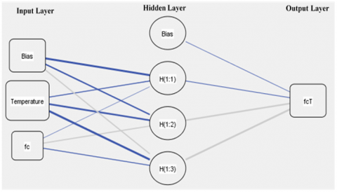
Table 4 presents the testing error ratios and correlation coefficients specifically for the middle layer, also known as the concealed layer. The values were obtained using a learning rate of 0.4 and a momentum coefficient of 0.9. The middle layer utilized the hyperbolic tangent as the transfer function, as shown in Table 3, it can be observed that the optimal performance of ANNs occurs when there are three neural nodes in the hidden layer. This configuration yields a maximum coefficient of correlation of 96.2% and the lowest error ratio of 6.2%. Thus, the result included of a total of two neural nodes in the input layer, three in the hidden layer, and one neural node in the output layer. These nodes indicate the anticipated compressive strength at higher temperatures (fcT).
The weights of a connection, which quantify the significance of the relationship between two neurons, are utilized to scale each input value from neurons in the preceding layer. The neuron subsequently accumulates all of these multiplications.
Upon completing the training of the ANNs, the weights of the neural nodes were acquired. Both the connections between the hidden layer and the output layer and the connections between the input layer and the hidden layer are represented by these weights. The layers are described in Figure 3, and Table 4 displays the weights of these connections as well as the output and hidden layer threshold limits.
Table 3. The impact of the hidden layer's node count on ANN performance
|
No. of Nodes |
Training Error (%) |
Testing Error (%) |
Coefficient Correlation (r) (%) |
|
1 |
7.9 |
10.2 |
93.6 |
|
2 |
15.1 |
11.8 |
89 |
|
3 |
13.4 |
6.2 |
96.2 |
|
4 |
9.1 |
8.3 |
95.1 |
|
5 |
7.8 |
21.9 |
96.3 |
Figure 3. The neural network architecture model
Table 4. The weights of connections
|
Predictor |
Predicted |
||||
|
Hidden Layer 1 |
Output Layer |
||||
|
H1-i |
H2-i |
H3-i |
Output |
||
|
Input Layer |
(Bias) |
0.090 |
-1.167 |
0.106 |
|
|
fc |
0.323 |
1.085 |
0.199 |
||
|
T |
-0.605 |
1.081 |
-0.435 |
||
|
Hidden Layer 1 |
(Bias) |
-0.715 |
|||
|
H1-i |
-0.902 |
||||
|
H2-i |
-1.018 |
||||
|
H3-i |
-0.587 |
||||
Importantly, during the training phase, all inputs (variables) (fc, T) have been transformed from their actual values to relative values in the range of (-1, 1) in compliance with the SPSS program's specifications. The weights (Wi) and threshold limit (Bias) listed in Table 4 were used to achieve this change. The following is the equation that is produced:
$H 1={Tanh}[0.001 * f c-0.063 * T+1.632]$ (3)
$H 2={Tanh}[0.003 * f c+0.114 * T-5.983]$ (4)
$H 3=T a n h[0.0005 * f c-0.046 * T+1.256]$ (5)
The variable (fcT) can be found in the following equation:
$Scale(f c T)={Tanh}[(-0.902 * H 1)-(1.018 * H 2)-(0.587 * H 3)-0.715]$ (6)
In order to acquire the actual values of outputs (fcT), Eq. (7) must be used to modify the relative value of the output. The value of the compressive strength at higher temperature (fcT) for NSC can be determined using Eq. (7):
$Unscale\left(f c T_{N S C}\right)=[ Scale (f c T) * D(f c T)]+A$ (7)
where, D(fcT)=(fcT Max.-fcT Min.) equal 18Mpa from experimental data. And D(fcT)=(fcT Max.-D(fcT)) equal to 21.6 MPa from experimental data.
In order to acquire the actual values of outputs (fcT), Eq. (8) must be used to modify the relative value of the output.
$Unscale\left(f c T \_N S C\right)=[18 * {Scale}(f c T)]+21.6$ (8)
When fc equals 31 MPa and T equals 309℃, Eqs. (3)-(7) are practically applied using one of the experimental results. As a result, the compressive strength at higher temperatures (fcT) for NSC is measured from Eqs. (3)-(8) is equal 27.1 MPa and the value experimental 27.9 MPa.
Statistical indicators such as mean absolute percentage error (MAPE), average accuracy percentage (AA%), coefficient of determination (R2), and correlation coefficient (R) were used by the validation model to evaluate the retrieved values. The efficacy of the equation obtained from the ANN model was assessed using these criteria. Eq. (9) was utilised to ascertain the MAPE value.
$M A P E=\frac{\left(\sum \frac{|A-E|}{A}\right) * 100}{n}$ (9)
where,
A: Actual values of (fcT).
E: The values of (fcT) are calculated by Eq. (8).
n: Number of samples.
The average accuracy percentage (AA %) value is calculated using Eq. (10).
$A A \%=100 \%-M A P E$ (10)
The statistical standards result for the validation model on 4 samples, or 8% of the total samples, are shown in Table 5. According to the findings, the formula used in the ANN model to calculate compressive strength at high temperatures (fcT) has an astounding 92.7% accuracy rate. The model established in the research is highly efficient, as evidenced by its great accuracy. Also, Figure 4 shows the agreement between the practical results and the proposed model.
Table 5. The result validation of ANNs model
|
Statistical Standards |
(R) |
Determination Coefficient (R2) |
MAPE (%) |
AA (%) |
|
Statistical value for ANNs model |
96.2 |
89.6 |
7.3 |
92.7 |
Figure 4. Agreement between the practical results and the proposed model
5.1.2 High-strength concrete HSC
Also, the input model consists of two independent variables: normal compressive strength (fc) and temperature (T). The output data is the high-strength concrete HSC at elevated temperature (fcT). The trial-and-error approach was employed to optimize the performance of the ANNs by maximizing the correlation coefficient (r) and minimizing testing mistakes. The data in Table 6 indicates that the training group has the greatest classification rate of 84%, while the testing group has a rate of 9% and the validation group has a rate of 7%. This conclusion is based on the lowest testing error ratio of 4.8% and the highest correlation coefficient of 97.2%.
Eq. (2) most can be used to determine the optimal number of neural nodes in ANNs in order to distribute the thirty-one samples across the three groups and attain the maximum number of neural nodes equal to 5. The correlation coefficients and testing error ratios for the middle layer, or concealed layer, of the high-strength concrete HSC at higher temperature (fcT) are shown in Table 6.
A learning rate of 0.4 and a momentum coefficient of 0.9 were used to get the values. The hyperbolic tangent function was used as the transfer function for the intermediate layer. As shown in Table 7, the ANNs perform best when the hidden layer consists of three neural nodes, achieving a maximum correlation coefficient of 97.2% and a minimum error rate of 4.8%. In order to depict the anticipated high-strength concrete HSC at enhanced temperature (fcT), ANNs developed a final model that included two neural nodes in the input layer, three neural nodes in the hidden layer, and one neural node in the output layer.
Table 6. The impact of data partitioning on ANN performance
|
Data Division |
Training Error (%) |
Testing Error (%) |
Coefficient Correlation (r) (%) |
||
|
Training (%) |
Testing (%) |
Validation (%) |
|||
|
60 |
10 |
30 |
4.3 |
11.4 |
95.3 |
|
60 |
20 |
20 |
6.3 |
9.1 |
94.9 |
|
60 |
30 |
10 |
8.1 |
7.8 |
96.6 |
|
70 |
10 |
20 |
9.1 |
5.2 |
96.2 |
|
70 |
20 |
10 |
4.9 |
30 |
96.3 |
|
80 |
10 |
10 |
14.4 |
15 |
94.7 |
|
84 |
9 |
7 |
6.4 |
4.8 |
97.2 |
Table 7. The impact of the hidden layer's node count on ANN performance
|
No. of Nodes |
Training Error (%) |
Testing Error (%) |
Coefficient Correlation (r) (%) |
|
1 |
8.9 |
10.8 |
94.6 |
|
2 |
14.7 |
10.7 |
94.8 |
|
3 |
6.4 |
4.8 |
97.2 |
|
4 |
10.5 |
7.3 |
95.8 |
|
5 |
17.8 |
21.0 |
94.9 |
Table 8. The weights of connections
|
Predictor |
Predicted |
||||
|
Hidden Layer 1 |
Output Layer |
||||
|
H1-i |
H2-i |
H3-i |
Output |
||
|
Input Layer |
(Bias) |
-0.515 |
0.145 |
-0.727 |
|
|
fc |
1.000 |
0.521 |
-0.221 |
||
|
T |
0.484 |
0.272 |
-1.405 |
||
|
Hidden Layer 1 |
(Bias) |
-0.646 |
|||
|
H1-i |
-1.223 |
||||
|
H2-i |
-0.735 |
||||
|
H3-i |
-1.219 |
||||
The final weights of a connection after training the model development by ANNs represent the importance of the correlation between two neurons. Table 8 also shows the weights of these connections, along with the output layer's and the hidden layer's threshold limits.
The training phase of SPSS needed all inputs (variables) (fc, T) to be converted to relative values between -1 and 1. This transformation uses weights (Wi) in Table 9 and threshold limit (Bias). The resulting equation is below:
$H 1={Tanh}[0.002 * f c+0.019 * T-3.296]$ (11)
$H 2={Tanh}[0.001 * f c+0.011 * T-1.367]$ (12)
$H 3=T a n h[-0.001 * f c-0.055 * T-3.994]$ (13)
$Scale(\mathrm{fcT})={Tanh}[(-0.646 * H 1)-(1.223 * H 2)-(0.735 * H 3)-0.219]$ (14)
$\mathrm{fcT}_{\mathrm{HSC}}=\lceil 41.1 * Scale (\mathrm{fcT})\rceil+43.4$ (15)
In the practical application of Eqs. (11)-(15) using one of the experimental data when fc, T equals 106Mpa and 350℃. As a result, the fcT_HSC is measured from Eqs. (11)-(15) is equal 71.66 MPa and the value experimental (70.47Mpa).
Table 9 displays the statistical standards findings for the validation model was tested on three samples, accounting for 7% of the total dataset. The findings indicate that the formula for predicting compressive strength at high temperatures (fcT) in the ANN model has a high accuracy of 88.8%. The model established in the research is highly efficient, as evidenced by its great accuracy. Also, Figure 5 shows the agreement between the practical results and the proposed model.
Table 9. The validation of the ANNs model's results
|
Statistical Standards |
(R) |
Determination Coefficient (R2) |
MAPE (%) |
AA (%) |
|
Statistical value for ANNs model |
97.2 |
90.3 |
11.2 |
88.8 |
Figure 5. Agreement between the practical results and the proposed model
5.2 Previous models vs. the proposed model
Recent computational approaches and methodologies for evaluating the fire performance of building structural elements have evolved. However, research on input information (material qualities) has lagged [7, 16]. The majority of ACI 216R-89 [31] is founded on studies conducted in the 1950s and 1960s, and it does not have a consistent link for high-temperature properties [7].
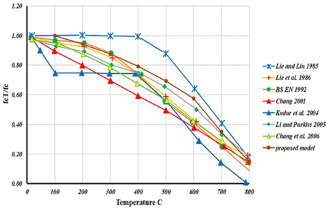
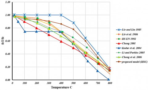
Analyze test results by comparing them to hypothesized relationships of compressive strength. Next, the proposed relationships between compressive and tensile stress and strain for NSC and HSC at elevated temperatures are compared to various experimental data from previous studies. Figures 6 to 8 show NSC and HSC compressive strength test results and models at different temperatures. Figure 6 compares Table 1 of models to the suggested NSC (20-45 MPa) connection at various temperatures using published unstressed experimental test findings [2-4, 6, 29, 30]. Unstressed tests heat the specimen constantly without pre-load until it reaches the desired temperature and thermal steady state.
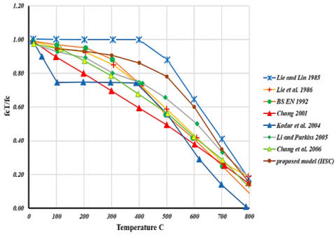
Figures 7 and 8 illustrate the comparisons between the models mentioned in Table 1 and the suggested correlation for HSC at different temperatures within the ranges of 55.2 to 80 MPa and 80 to 110 MPa, respectively, with previously published experimental results without any applied stress [2-6]. The hypothesized correlation closely corresponds to the test outcomes for NSC and HSC, which were generated using ANNs.
Figure 6. Comparison between NSC (20-45 MPa) at elevated temperatures with the proposed model
Figure 7. Comparison between HSC (50-80Mpa) at elevated temperatures with the proposed model
Figure 8. Comparison between HSC (80-110 MPa) at elevated temperatures with the proposed model
(1) The bulk of compressive strength correlations available are unreliable for measuring NSC and HSC at high temperatures. Compressive strength and concrete at high temperatures are linked using a modified ANN model.
(2) The proposed model has two inputs (fc and T). In contrast, previous models were based on one variable (T) and this variable, through data analysis in the current research, proved that there is a change in (fc) with (T) whenever the amount of (fc) changes by ten units (10 MPa).
(3) The neural network method ANN was employed to predict the behavior of the NSC and HSC at high temperatures. The predictions achieved an average accuracy of 92.7% and a correlation coefficient of 96.2% for the NSC, and an average accuracy of 88.8% and a correlation coefficient of 97.2% for the HSC.
(4) NSC loses 10-20% from fc at 300°C and 60-75% at 600℃. The models described by Lie and Lin [26] and Lie et al. [27] provide the upper and lower bounds for fc′T. Also, HSC loses 40% from fc up to 450℃.
(5) This research emphasizes the necessity of conducting additional experiments at various temperatures to examine the influence of compressive strength on both NSC and HSC.
(6) The possibility of building an ANN model for lightweight concrete LWC exposed to high temperatures through previous research data.
The authors would like to thank University of Samarra (https://uosamarra.edu.iq/) in Salah Al-Deen-Iraq, and Mustansiriyah University (www.uomustansiriyah.edu.iq) in Baghdad-Iraq for its support in the present work.
[1] Bastami, M., Aslani, F., Esmaeilnia, O.M. (2010). High-Temperature mechanical properties of concrete. International Journal of Civil Engineering, 8(4): 337-351.
[2] Castillo, C. (1987). Effect of transient high temperature on high-strength concrete. Rice University.
[3] Diederichs, U., Ehm, C., Weber, A., Becker, A. (1987). Deformation behaviour of HRT concrete under biaxial stress and elevated temperatures. In Proceedings of the Ninth International Conference on Structural Mechanics in Reactor Technology, pp. 17-21.
[4] Flynn, D.R. (1999). Response of high performance concrete to fire conditions: Review of thermal property data and measurement techniques. Millwood, Va, USA: National Institute of Standards and Technology, pp. 119-134.
[5] Poon, C.S., Azhar, S., Anson, M., Wong, Y.L. (2003). Performance of metakaolin concrete at elevated temperatures. Cement and Concrete Composites, 25(1): 83-89. https://doi.org/10.1016/S0958-9465(01)00061-0
[6] Sancak, E., Sari, Y.D., Simsek, O. (2008). Effects of elevated temperature on compressive strength and weight loss of the light-weight concrete with silica fume and superplasticizer. Cement and Concrete Composites, 30(8): 715-721. https://doi.org/10.1016/j.cemconcomp.2008.01.004
[7] Kodur, V.K., Dwaikat, M.M.S., Dwaikat, M.B. (2008). High-temperature properties of concrete for fire resistance modeling of structures. ACI Materials Journal, 105(5): 517.
[8] Naus, D.J. (2006). The effect of elevated temperature on concrete materials and structures-A Literature Review. https://doi.org/10.2172/974590
[9] Phan, L.T., Carino, N.J. (1998). Review of mechanical properties of HSC at elevated temperature. Journal of Materials in Civil Engineering, 10(1): 58-65. https://doi.org/10.1061/(ASCE)0899-1561(1998)10:1(58)
[10] Phan, L.T., Carino, N.J. (2003). Code provisions for high strength concrete strength-temperature relationship at elevated temperatures. Materials and Structures, 36: 91-98. https://doi.org/10.1007/BF02479522
[11] Ali, S.I., Ahmed, A.M., Ibrahim, A.E., Ali, M.I. (2024). Effect of utilization waste strapping plastic belts on flexural behaviour of concrete. Annales de Chimie - Science des Matériaux, 48(1): 95-100. https://doi.org/10.18280/acsm.480111
[12] Bisby, L., Gales, J., Maluk, C. (2013). A contemporary review of large-scale non-standard structural fire testing. Fire Science Reviews, 2: 1-27. https://doi.org/10.1186/2193-0414-2-1
[13] Aslani, F., Bastami, M. (2011). Constitutive relationships for normal-and high-strength concrete at elevated temperatures. ACI Materials Journal, 108(4): 355.
[14] Karataş, M., Benli, A., Ergin, A. (2017). Influence of ground pumice powder on the mechanical properties and durability of self-compacting mortars. Construction and Building Materials, 150: 467-479. https://doi.org/10.1016/j.conbuildmat.2017.05.220
[15] Phan, L.T., Phan, L.T. (1996). Fire performance of high-strength concrete: A report of the state-of-the art. Gaithersburg, MD: US Department of Commerce, Technology Administration, National Institute of Standards and Technology, Office of Applied Economics, Building and Fire Research Laboratory, Vol. 105.
[16] Kodur, V.K.R., Harmathy, T.Z. (2016). Properties of building materials. In SFPE Handbook of Fire Protection Engineering, pp. 277-324. https://doi.org/10.1007/978-1-4939-2565-0_9
[17] Ahmed, A.M., Ali, S.I., Ali, M.I., Jamel, A.A.J. (2023). Analyzing self-compacted mortar improved by carbon fiber using artificial neural networks. Annales de Chimie - Science des Matériaux, 47(6): 363-369. https://doi.org/10.18280/acsm.470602
[18] Jamel, A.A.J., Ali, M.I. (2021). Stability and seepage of earth dams with toe filter (Calibrated with artificial neural network). Journal of Engineering Science and Technology, 16(5): 3712-3725.
[19] Abu-Alsaad, H.A. (2019). Agent applications in e-learning systems and current development and challenges of adaptive e-Learning systems. In 2019 11th International Conference on Electronics, Computers and Artificial Intelligence (ECAI), Pitesti, Romania, pp. 1-6. https://doi.org/10.1109/ECAI46879.2019.9042015
[20] Ali, M.I., Jamel, A.A.J., Ali, S.I. (2020). The hardened characteristics of self-compacting mortar including carbon fibers and estimation results by artificial neural networks. AIP Conference Proceedings, 2213(1). https://doi.org/10.1063/5.0000177
[21] AbuAlsaad, H.A., AlTaie, R. (2018). Using big data technology for prediction of quiz difficulty level in E-learning systems. Iraqi Journal of Information Technology, 8(4).
[22] Graupe, D. (2013). Principles of artificial neural networks. World Scientific, Vol. 7.
[23] Abu-Alsaad, H.A. (2023). CNN-based smart parking system. International Journal of Interactive Mobile Technologies, 17(11). https://doi.org/10.3991/ijim.v17i11.37033
[24] Abu-Alsaad, H.A., Al-Taie, R.R.K. (2024). Smart parking system using IoT. In 2024 16th International Conference on Electronics, Computers and Artificial Intelligence (ECAI), Iasi, Romania, pp. 1-7. https://doi.org/10.1109/ECAI61503.2024.10607419
[25] Schneider, U. (Ed.). (1985). Properties of materials at high temperatures concrete. Gesamthochsch. Bibliothek. https://firedoc.nist.gov/article/6XcxXYQBWEcjUZEYug11.
[26] Lie, T.T., Lin, T.D. (1985). Fire performance of reinforced concrete columns. ASTM International, pp. 176-205.
[27] Lie, T.T., Rowe, T.J., Lin, T.D. (1986). Residual strength of fire-exposed reinforced concrete columns. Special Publication, 92: 153-174. https://doi.org/10.14359/6517
[28] Designers' guide to EN 1992-I-I and EN 1992-1-2 Eurocode 2: Design of concrete structures. General rules and rules for buildings and structural fire design, 2005. https://books.google.iq/books?hl=ar&lr=&id=9Ua7KKD-4FEC&oi=fnd&pg=IA3&dq=Design+of+concrete+structures-Part+1-2:+General+rules-Structural+fire+design.+1995,+ENV+1992-1-2.&ots=7q50D1mt1Z&sig=9uQKDMO89On05NwS8Wq_FpHozTA&redir_esc=y#v=onepage&q&f=false.
[29] American Society of Civil Engineers. (1992). Structural fire protection. In Manual No. 78, ASCE Committee on Fire Protection, Structural Division, New York. https://doi.org/10.1061/9780872628885
[30] Lie, T., Erwin, R. (1993). Method to calculate the fire resistance of reinforced concrete columns with rectangular cross section. ACI Structural Journal, 90(1): 52-60. https://www.safetylit.org/citations/index.php?fuseaction=citations.viewdetails&citationIds=citjournalarticle_42970_34.
[31] Chang, C.H., Jau, W.C. (2001). Study of fired concrete strengthened with confinement. Hsinchu: National Chiao Tung University.
[32] Kodur, V.K.R., Wang, T.C., Cheng, F.P. (2004). Predicting the fire resistance behavior of high strength concrete columns. Cement and Concrete Composites, 26(2): 141-153. https://doi.org/10.1016/S0958-9465(03)00089-1
[33] Li, L., Purkiss, J.A. (2005). Stress-strain constitutive equations of concrete material at elevated temperatures. Fire Safety Journal, 40(7): 669-686. https://doi.org/10.1016/j.firesaf.2005.06.003
[34] Chang, Y.F., Chen, Y.H., Sheu, M.S., Yao, G.C. (2006). Residual stress-strain relationship for concrete after exposure to high temperatures. Cement and Concrete Research, 36(10): 1999-2005. https://doi.org/10.1016/j.cemconres.2006.05.029
[35] Bastami, M., Aslani, F., Esmaeilnia, O.M. (2010). High-temperature mechanical properties of concrete. International Journal of Civil Engineering, 8(4). https://scholar.googleusercontent.com/scholar?q=cache:Rjf45SGS5RMJ:scholar.google.com/+%5B35%5D%09Bastami,+M.,+F.+Aslani,+and+O.M.+Esmaeilnia,+High-temperature+mechanical+properties+of+concrete.+2010.&hl=ar&as_sdt=0,5.