Awatif Muflih Alqahtani![]() | Hamza Mihoubi*
| Hamza Mihoubi*![]()
© 2025 The authors. This article is published by IIETA and is licensed under the CC BY 4.0 license (http://creativecommons.org/licenses/by/4.0/).
OPEN ACCESS
The aim of the paper is to present a numerical technique that applies the homotopy perturbation method to solve the time-Fractional Black-Scholes European option pricing equation with boundary conditions. The study employs the $\varphi-$Caputo Fractional derivative in time, and the operator admits as particular cases the Caputo and Caputo–Hadamard Fractional derivatives describe the solutions of these equations that contribute to the generalization and development of certain recent results. The method offers a convergent series with easily computed components as an analytical solution. The method outperforms currently available analytical techniques without the need for linearization or minor perturbations. The homotopy perturbation approach is a practical and efficient way to get over the limitations of more conventional techniques, as demonstrated by the two examples presented under Caputo–Hadamard memory, when applied to the time-Fractional Black-Scholes European option pricing equation, the techniques' accuracy and ease of implementation are demonstrated by the numerical findings.
φ-Caputo Fractional derivative, Caputo–Hadamard Fractional derivative, homotopy perturbation method, Mittag–Leffler function, Fractional Black-Scholes European option pricing equation
The well-known theoretical option value model was developed in 1973 by Black and Scholes [1]. Their methodology is based on the premise of building a risk-free portfolio by investing in cash bonds, options, and the underlying stock. As a result, the Black-Scholes formula is frequently employed as a model to value American options, which can be exercised at any time up to the stock's expiration date, and European options, which can only be exercised on a given future date [2]. To obtain a closed form solution for the Black-Scholes equation, one must first solve the heat equation fundamentally. Consequently, it is crucial to adjust some variables at this point in order to convert the B-S equation into the heat equation. It is possible to convert the closed form solution of the heat equation back into the appropriate-solution of the Black-Scholes partial differential equation. Financial models were generally formulated utilizing stochastic differential equations. Nevertheless, it was quickly shown that these models may be described as linear evolutionary PDE with changing coefficients under specific circumstances [3]. Thus, the following equation the equation represents the Black-Scholes model, which calculates an option's value:
$\begin{gathered}\frac{\partial U(x, t)}{\partial t}+\frac{\sigma^2 x^2}{2} \frac{\partial^2 U(x, t)}{\partial x^2}+r(t) x \frac{\partial U(x, t)}{\partial x}-r(t) U=0,(t, x) \in \mathbb{R}^{+} \times(0, T)\end{gathered}$ (1)
where, T is the maturity date, K is the exercise price, $r(t)$ is the risk-free interest rate, and $\sigma(x, t)$ is the volatility function of the underlying asset. $U(x, t)$ is the price of a European call option at asset price $x$ and at time $t$. The values of the European call and put options will be shown by the variables $U_C(x, t)$ and $U_p(x, t)$, respectively. The payout mechanisms consist of:
$\begin{aligned} U_C(x, t) & =\max (x-E, 0), U_p(x, t) =\max (E-x, 0)\end{aligned}$ (2)
In this case, the function $\max (x, 0)$ produces the greater value between $x$ and 0, where $E$ represents the options' expiration price. Over the last few decades, numerous scholars have examined the possibility of Black-Scholes model solutions using a variety of techniques [4-12]. Fractional differential equations also provide an excellent description of many important phenomena in the disciplines of electromagnetic, acoustics, viscoelasticity, electrochemistry, and material science [13-15]. Oldham and Spanier's book [16] has been significant in the field's advancement. The following sources contain some basic findings about solving fractional differential equations: Miller [17], Podlubny [18], Kilbas et al. [19], and Podlubny [20]. In order to achieve analytic and approximate solutions for fractional BS equations, this study aims to expand the application of the homotopy perturbation method (HPM) under Caputo-Hadamard memory. The homotopy perturbation method was initially introduced and used by a mathematician from He [21-25]. Yıldırım and Koçak [26] successfully adapted the approach to the space time fractional advection - dispersion problem. Fractional KdV equation by Abdulaziz et al. [27], fractional Zakharov-Kuznetsov equations by Yildirim and Gülkanat [28]. Khan et al. [29] fractional chemical engineering equation. The homotopy perturbation method [30-34] is one of the very applicable analytical approaches. Numerous nonlinear problems are solved using this approach [35-39], and the references therein cover a broad range of linear and nonlinear, homogeneous and inhomogeneous scientific and engineering applications.
The Fractional Black-Scholes equation can be expressed as follows:
$\begin{array}{r}{ }_t^C \mathcal{D}_a^{\alpha: \varphi} U(x, t)+\frac{\sigma^2 x^2}{2} \frac{\partial^2 U(x, t)}{\partial x^2}+r(t) x \frac{\partial U(x, t)}{\partial x}-r(t) U=0, \quad 0<\alpha \leq 1\end{array}$ (3)
Equipped with the terminal and boundary condition:
$\begin{gathered}U(x, T)=\max (x-E, 0), x \in \mathbb{R}^{+}, U(0, t)=0, t \in[0, T]\end{gathered}$ (4)
Numerous novel kinds of fractional derivatives have been put out, studied, and used in real-world models in recent years. It is therefore normal to attempt to merge those ideas into a single one. Developing the foundations of a theory for fractional differential equations with a general derivative is crucial. In this research, we chose the $\varphi$-Caputo Fractional derivative in time whose operator admits as particular cases the Caputo and Caputo-Hadamard Fractional derivatives to solve the time-Fractional Black-Scholes European option pricing equation utilizing homotopy perturbation method it was created to deal with fractional differential equations, which are common in engineering and science. Its ability to produce quickly convergent series solutions for fractional partial differential equations is its primary benefit. We seek to find both analytical and numerical solutions of the time-Fractional Black-Scholes European option pricing equation. Consequently, the numerical results are presented through the graphical illustrations. The solution is provided by the proposed method in a quickly converging series, which may ultimately lead to both an exact and approximate solution. This research paper is divided as follows: In Section 2, basic ideas related to the characteristics and notations of fractional calculus are explored, which are pertinent to the topics covered in this work. In Section 3, we employ the homotopy perturbation method approach to derive solutions for the time-fractional B-S equation. In Section 4, we apply the proposed method to the time-fractional B-S equation to verify the effectiveness and accuracy of this method under Caputo-Hadamard memory. We present the results through graphical and numerical analyses. Finally, Section 5 presents the conclusions drawn from our results.
Mathematics' propensity toward potential generalization is a crucial feature of the 20th century. The first conference devoted solely to the fractional calculus* and its applications in various* fields of knowledge brought significant attention to the introduction of new mathematical concepts as well as the generalization of existing ones. Two such concepts were the fractional/integral and the fractional/derivative [40]. Numerous versions of the fractional derivative operator, referred to as the Riemann-Liouville, Günwald-Letnikov, and Caputo derivatives, were introduced. We are interested in a specific variant of the Caputo derivative in this study. Later in the 20th century, Gerasimov and Dzerbashian retrieved and shared it, and Caputo was the one who suggested studying it in order to apply it with the Laplace/ transform. For a fractional calculus, Reference [41] provides a recent fractional calculus chronology. This section provides an overview of the definitions/ and characteristics of the fractional derivatives and integrals of a function f in relation to another function φ. References [19, 42] provide definitions and attributes for some of these terms.
This section contains some of the φ-Caputo Fractional derivative [42] notations, definitions, lemmas, and results that are utilized throughout the paper.
Definition 2.1 [19, 42]: Let f be an integrable function defined on $I, \varphi \in C^1(I)$ be a growing function such that $\varphi^{\prime}(t) \neq 0$ for every $t \in I$, and let $\alpha>0, I=[a, b]$ be a finite or infinite interval. In relation to another function $\varphi$ of order α, the definition of the left fractional integral of f is
$\begin{gathered}\mathcal{J}_a^{\alpha ; \varphi}[f(x, t)] =\frac{1}{\Gamma(\alpha)} \int_a^t \varphi^{\prime}(\mu)(\varphi(t)-\varphi(\mu))^{\alpha-1} f(x, \mu) d \mu\end{gathered}$ (5)
The Riemann-Liouville fractional integral is obtained if $\varphi(t)=t$, while the Hadamard fractional integral is obtained if $\varphi(t)=\ln t \quad$ [19]. Assuming $\alpha=0$, we obtain $\mathcal{J}_a^{0 ; \varphi}[f(x, t)]=f(x, t)$.
Theorem 2.1 [40]:
Let $\alpha>0, n \in \mathbb{N}, I$ is the interval $-\infty \leq a<\infty$, and $f, \varphi \in$ $C^n(I)$ two functions such that $\varphi$ is increasing and $\varphi^{\prime}(t) \neq 0$, for all $t \in I$. The left $\varphi$-Caputo fractional derivative of f of order α is given by:
${ }_t^C \mathcal{D}_a^{\alpha ; \varphi}[f(x, t)]=\mathcal{J}_a^{n-\alpha ; \varphi}\left(\frac{1}{\varphi^{\prime}(t)} \frac{\partial}{\partial t}\right)^n f(x, t)$ (6)
where,
$n=[\alpha]+1$ for $\alpha \notin \mathbb{N}, n=\alpha$ for $\alpha \in \mathbb{N}$.
We shall utilize the shortened notation to make the notation simpler.
$f^{[n] ; \varphi}(x, t)=\left(\frac{1}{\varphi^{\prime}(t)} \frac{\partial}{\partial t}\right)^n f(x, t)$ (7)
In the event when $\varphi(t)=t$, the Caputo fractional derivative is obtained [43], while the Caputo-Hadamard Fractional derivative is obtained if $\varphi(t)=\ln t$ [44].
We introduce the Caputo-type Hadamard Fractional derivatives, as follows:
Theorem 2.2 [44]: Let $\Re(\alpha) \geq 0, n=[\Re(\alpha)]+1$. If $f \in C_\delta^n([a, b])$, where $0<a<b<\infty$, and
$\begin{gathered}A C_\delta^n([a, b])= \\ \left\{g:[a, b] \rightarrow \mathbb{C}: \delta^{n-1} g(x) \in A C[a, b], \delta=x \frac{d}{d x}\right\}\end{gathered}$
then ${ }_t^{{ }_t} \mathcal{D}_a^{\alpha ; \varphi} f(t)$ exist everywhere on [a, b]:
${ }_t^{C} \mathcal{D}_a^{\alpha ; \varphi} f(t)=\frac{1}{\Gamma(n-\alpha)} \int_a^t\left(\ln \frac{t}{\xi}\right)^{n-\alpha-1}\left(t \frac{d}{d t}\right)^n f(\xi) \frac{d \xi}{\xi}$
Lemma 2.1 [44]: Let $f \in C([a, b]), \Re(\alpha)>0, n=[\Re(\alpha)]+1$ if $\Re(\alpha) \neq$ or $\alpha \in \mathbb{N}$, then
${ }_t^C \mathcal{D}_a^{\alpha ; \varphi} \mathcal{J}_a^{\alpha ; \varphi} f(t)=f(t)$.
Lemma 2.2 [44]: Let $f \in A C^n([a, b])$, and $\alpha \in \mathbb{C}$, then
$\mathcal{J}_a^{\alpha ; \varphi}{ }_t \mathcal{D}_a^{\alpha ; \varphi} f(t)=f(t)-\sum_{k=0}^{n-1} \frac{\delta^k f(a)}{k!}\left(\ln \frac{t}{a}\right)^k$
Theorem 2.3 [42]: Let $f \in C^n([a, b])$, and $n-1<\alpha \leq n, n \in \mathbb{N}, \eta>0$, then
Definition 2.2 [45]: Let $\alpha, m>0$. The power series represents the one-parameter Mittag-Leffler function.
$\mathrm{E}_{\alpha, m}(t)=\sum_{m=0}^{\infty} \frac{t^m}{\Gamma(m \alpha+1)}$ (8)
where, $\Gamma(.)$ is gamma function.
The following analysis of the fractional-order nonlinear non homogeneous partial differential equation with starting conditions (IC) illustrates the fundamental concept of the homotopy perturbation method:
$\begin{gathered}{ }_t^C \mathcal{D}_a^{\alpha ; \varphi} u(x, t)+R u(x, t)+N u(x, t)=g(x, t), \\ 0<\alpha \leq 1\end{gathered}$ (9)
subject to IC:
$u^{(k)}(x, 0)=h_k(x), k=0,1, \ldots, n-1$ (10)
where, $g(x, t)$ is the source term, R and N stand for linear and nonlinear differential operators, respectively, ${ }_{\mathrm{t}}^C \mathcal{D}_{\mathrm{a}}^{\alpha ; \varphi}=\frac{\partial^\alpha}{\partial \mathrm{t}{ }^\alpha}$, for the differential operator, and ${ }_{\mathrm{t}}^C \mathcal{D}_{\mathrm{a}}^{\alpha ; \varphi} \mathrm{u}(\mathrm{x}, \mathrm{t})$ for the derivative of $u(x, t)$ of the Caputo type [46].
$\begin{aligned}{ }_t^C \mathcal{D}_a^{\alpha ; \varphi} u(x, t)+p & (R u(x, t)+N u(x, t)-g(x, t)) \\ & =0, \quad 0<\alpha \leq 1\end{aligned}$ (11)
where, the embedding parameter is $p \in[0,1]$. When $p=0$, Eq. (11) turn into:
${ }_t^C \mathcal{D}_a^{\alpha ; \varphi} u(x, t)=0$ (12)
and Eq. (11), when p=1, prove to be the original Eq. (9).
Initially, we must take into account the following series form solution with the embedding parameter $p \in[0,1]$:
$u(x, t)=\sum_{n=0}^{\infty} p^n u_n(x, t)$ (13)
and He's polynomials can be used to decompose the nonlinear term as follows:
$N u(x, t)=\sum_{n=0}^{\infty} p^n H_n(u)$ (14)
where, $H_n(u)$ is He’s polynomials [47] and is given by:
$\begin{gathered}H_n\left(u_0, u_1, u_2, \ldots u_n\right)= \\ \frac{1}{n!} \frac{\partial}{\partial p^n}\left[N \sum_{n=0}^{\infty} p^n u_n(x, t)\right]_{p=0}, n=1,2,3, \ldots\end{gathered}$ (15)
Substituting Eqs. (13) and (14) in Eq. (11), we get:
$\begin{array}{r}{ }_t^{C} \mathcal{D}_a^{\alpha_{;} \varphi}\left[\sum_{n=0}^{\infty} p^n u_n(x, t)\right] =p\left[g(x, t)-R \sum_{n=0}^{\infty} p^n u_n(x, t)-N \sum_{n=0}^{\infty} p^n H_n(u)\right]\end{array}$ (16)
The following approximations can be obtained successively by contrasting the coefficients on both sides of Eq. (15) for the same powers of p.
$p^0:{ }_t^C \mathcal{D}_a^{\alpha ; \varphi}\left[u_0(x, t)\right]=0$ (17)
$p^1:{ }_t^C \mathcal{D}_a^{\alpha ; \varphi}\left[u_1(x, t)\right]=g(x, t)-R u_0(x, t)-N H_0(u)$ (18)
$p^2:{ }_t^C \mathcal{D}_a^{\alpha ; \varphi}\left[u_2(x, t)\right]=-R u_1(x, y, t)-N H_1(u)$ (19)
$\begin{array}{r}p^3:{ }_t^C \mathcal{D}_a^{\alpha ; \varphi}\left[u_3(x, t)\right]=-R u_2(x, t)-N H_2(u), \\ \vdots \quad\quad\quad\quad \quad \vdots \quad \quad \quad \quad \quad \quad\quad \quad\vdots \quad\quad\quad\\ p^n:{ }_t^C \mathcal{D}_a^{\alpha ; \varphi}\left[u_n(x, t)\right]=-R u_{n-1}(x, t)-N H_{n-1}(u)\end{array}$ (20)
The first few terms of the homotopy perturbation method solution can be expressed as follows by using the operator $\mathcal{J}_a^{\alpha ; \varphi}$, the inverse operator of ${ }_t^C \mathcal{D}_a^{\alpha ; \varphi}$ that is given in the preceding chapter, on both sides of the equations indicated above, and by the use of the IC in Eq. (10).
$u_0(x, t)=\sum_{k=0}^{n-1} u^k(x) \frac{t^k}{k!}=\sum_{k=0}^{n-1} g_k(x) \frac{t^k}{k!}$ (21)
$\begin{gathered}u_1(x, t)=\mathcal{J}_a^{\alpha ; \varphi}[g(x, t)] -\mathcal{J}_a^{\alpha ; \varphi}\left[R u_0(x, t)\right]-\mathcal{J}_a^{\alpha ; \varphi}\left[N H_0(u)\right]\end{gathered}$ (22)
$u_2(x, t)=J_a^{\alpha ; \varphi}\left[R u_1(x, t)\right]-J_a^{\alpha ; \varphi}\left[N H_1(u)\right]$ (23)
and so forth. Thus, the solution to Eq. (9) can be found as:
$\begin{aligned} u(x, t)= & \lim _{n \rightarrow \infty} u_n(x, t)=u_0(x, t)+u_1(x, t)+u_2(x, t)+u_3(x, t)+\cdots\end{aligned}$ (24)
3.1 Convergence analysis and error estimation
These two theorems prove the convergence of the homotopy perturbation technique towards a solution for the time-Fractional Black-Scholes equation and the error estimation of the homotopy perturbation method. With $0<T \leq \infty$, let $T$ be a positive constant and $\Omega \in \mathbb{R}^n$ be an opened and bounded domain. In order to demonstrate the HPM approach concept, let's look at the F B-S equation for any $(\mathrm{x}, \mathrm{t}) \in \Omega \times[0, \mathrm{~T}]$.
Theorem 3.1 [48]:
Let $u_n(x, t)$ be the function in a Banach space $C(\Omega \times$ $[0, T])=\{\mathrm{u}$ such that u is continuous on $\Omega \times$ $[0, T]\}$ defined by Eq. (24) for any $n \in \mathbb{N}$. The infinite series $\sum_{k=0}^{\infty} u_k(x, t)$ converges to the solution $u$ of Eq. (9) if there exists a constant $0<\mu<1$ such that $u_n(x, t) \leq \mu u_{n-1}(x, t)$ for all $n \in \mathbb{N}$. Thus, $\left\{S_n\right\}_{n=0}^{\infty}$ is a Cauchy sequence in the Banach space $C^n([a, b], \mathbb{R})$; consequently, the solution $\sum_{k=0}^{\infty} u_k(x, t)$ converge to $u$.
The following is the theorem we use to truncate an imprecise solution:
Theorem 3.2 [48]: The series solution's highest absolute error, defined in Eq. (35), is assessed as follows:
$\left|u(x, t)-\sum_{k=0}^{\infty} u_k(x, t)\right| \leq\left(\frac{\mu^{m+1}}{1-\mu}\right)\left\|u_0\right\|$ (25)
In this part, we solve Fractional Black-Scholes using the homotopy2perturbation technique Eq. (1).
4.1 Application 1
Consider the following Fractional Black-Scholes equation:
${ }_t^C \mathcal{D}_a^{\alpha ; \varphi} U(x, t)=\frac{\partial^2 u}{\partial x^2}+(k-1) \frac{\partial u}{\partial x}-k U, 0<\alpha \leq 1, t \geq 0, x \in \mathbb{R}$ (26)
With IC:
$U(x, 0)=\max \left(e^x-1,0\right)$ (27)
Let's build the homotopy of Eq. (26) in accordance with Eq. (11) as follows:
${ }_t^C \mathcal{D}_a^{\alpha ; \varphi} U(x, t)=p\left(\frac{\partial^2 u}{\partial x^2}+(k-1) \frac{\partial u}{\partial x}-k U\right)$ (28)
Substituting Eqs. (13) and (14) into Eq. (28), where, $H_n(U)$ are He’s polynomials which signify the nonlinear terms.
$\begin{gathered}H_n(U)=H_n\left(U_0, U_1, U_2, \ldots U_n\right) =\frac{1}{n!} \frac{\partial}{\partial p^n}\left[N \sum_{n=0}^{\infty} p^n U_n\right] \mathrm{n}=0,1,2,3, \ldots\end{gathered}$ (29)
The first few components of He’s polynomialsare given as follows:
$H_n(U)=\frac{\partial^2 U_n}{\partial x^2}+(k-1) \frac{\partial U_n}{\partial x}-k U_n, n \in N$
The following expressions result from gathering the like power of p:
$\begin{gathered}p^0:{ }_t^C \mathcal{D}_a^{a ; \varphi} U_0(x, t)=0, \\ p^1:{ }_t^C \mathcal{D}_a^{\alpha ; \varphi} U_1(x, t)=\frac{\partial^2 U_0}{\partial x^2}+(k-1) \frac{\partial U_0}{\partial x}-k U_0, \\ p^2:{ }_t^C \mathcal{D}_a^{\alpha ; \varphi} U_2(x, t)=\frac{\partial^2 U_1}{\partial x^2}+(k-1) \frac{\partial U_1}{\partial x}-k U_1,\end{gathered}$
$\begin{gathered}p^3:{ }_t^C \mathcal{D}_a^{\alpha ; \varphi} U_3(x, t)=\frac{\partial^2 U_2}{\partial x^2}+(k-1) \frac{\partial U_2}{\partial x}-k U_2, \\ \vdots \quad\quad\quad\quad \vdots\quad\quad\quad\quad \vdots \\ p^n:{ }_t^C \mathcal{D}_a^{\alpha ; \varphi} U_n(x, t)=\frac{\partial^2 U_{n-1}}{\partial x^2}+(k-1) \frac{\partial U_{n-1}}{\partial x}-k U_{n-1},\end{gathered}$
Utilizing the in initial condition Eq. (27), we have the following after applying the operator $\mathcal{J}_a^{\alpha ; \varphi}$ on both sides of the previously described expressions:
$\begin{gathered}p^0: U_0(x, t)=\max \left(e^x-1,0\right), \\ p^1: U_1(x, t)=-\max \left(e^x, 0\right) \frac{-k(\varphi(t)-\varphi(a))^\alpha}{\Gamma(\alpha+1)}+\max \left(e^x\right.-1,0) \frac{-k(\varphi(t)-\varphi(a))^\alpha}{\Gamma(\alpha+1)},\end{gathered}$
$\begin{aligned} p^2: U_2(x, t)=- & \max \left(e^x, 0\right) \frac{k^2(\varphi(t)-\varphi(a))^{2 \alpha}}{\Gamma(2 \alpha+1)}+\max \left(e^x\right. -1,0) \frac{k^2(\varphi(t)-\varphi(a))^{2 \alpha}}{\Gamma(2 \alpha+1)}, \\ p^3: U_3(x, t)=- & \max \left(e^x, 0\right) \frac{k^3(\varphi(t)-\varphi(a))^{3 \alpha}}{\Gamma(3 \alpha+1)}+\max \left(e^x\right. -1,0) \frac{k^3(\varphi(t)-\varphi(a))^{3 \alpha}}{\Gamma(3 \alpha+1)}, \\ & \vdots \quad \quad \quad \vdots \quad\quad\quad \vdots \end{aligned}$
In consequence, the solutions $U(x, t)$ are written in the form of:
$\begin{array}{r}U(x, t)=U_0(x, t)+U_1(x, t)+U_2(x, t)+U_3(x, t) +\cdots=\max \left(e^x, 0\right)-\max \left(e^x, 0\right)\end{array}$ (30)
Lastly, we write infinite sums in terms of the Mittag-Leffler function. Eq. (8) looks like this:
$\begin{gathered}U(x, t)= \max \left(e^x, 0\right)\left(1-\mathbb{E}_\alpha\left(-k(\varphi(t)-\varphi(a))^\alpha\right)\right) +\max \left(e^x-1,0\right) \mathbb{E}_\alpha\left(-k(\varphi(t)-\varphi(a))^\alpha\right)\end{gathered}$ (31)
This solution leads us to the conclusion that Eq. (31). Has two significant special instances. Initially, assuming $\varphi(t)=t$, and $\alpha=1$ (This is the fractional integral of RiemannLiouville) $a=0$. The exact solution in this case is as follows:
$\begin{gathered}U(x, t)=\max \left(e^x, 0\right)\left(1-\mathbb{E}_\alpha(-k t)\right)+\max \left(e^x-1,0\right) \mathbb{E}_\alpha(-k t)\end{gathered}$ (32)
Which is in full agreement with the results acquired by Edeki et al. [49] through the use of the projected differential transformation method (PDTM) and are alike in agreement with the solutions found by Saratha et al. [50] using fractional generalized homotopy analysis approach (FGHAM). On the other hand, if $\varphi(t)=\ln t$, (we have the Hadamard fractional integral) $a>0$, Eq. (31) yields a solution that becomes:
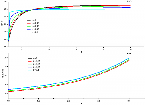
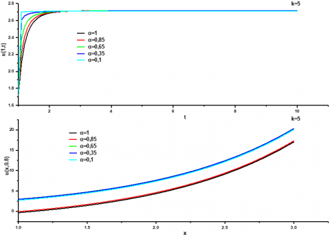
$\begin{aligned} U(x, t) & =\max \left(e^x, 0\right)\left(1-\mathbb{E}_\alpha\left(-k\left(\ln \frac{t}{a}\right)^\alpha\right)\right) \\ + & \max \left(e^x-1,0\right) \mathbb{E}_\alpha\left(-k\left(\ln \frac{t}{a}\right)^\alpha\right)\end{aligned}$ (33)
(a)
(b)
Figure 1. The graphs of Eq. (33) different value of parameter α with, a=1, α=1, 0.85,0.65, 0.35, 0.1
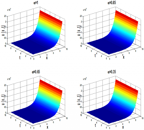
Figure 2. Surface shows the behavior of solution U(x, t) of application 1 using Eq. (33) with respect to t and x with α=1, α=0.85, α=0.65, α=0.35
Solution plots of Eq. (33) is shown in Figure 1 for the different fractional parameter settings of α=0.85, 0.65, 0.35, 0.1 and 1, respectively. Financial pricing derivatives according to various fractional parameter settings (α=0.85, 0.65, 0.35, 0.1 and 1) are shown in Figure 2.
In Table 1, the convergence of the series solution of Eq. (26) is demonstrated by Table 1, which also displays numerical values for various values of $\alpha$ and $\varphi(\mathrm{t})=lnt$. They also show the absolute errors with respect to specific different values of t and $\alpha=1$ as well as the solution obtained by the homotopy perturbation method and the exact solution Eq. (32).
Table 1. Numerical values of the approximate and exact solutions Eq. (32) to applications 1 for different values of $t$, and $x=1$, and α=1, α=0.85, α=0.65
|
t |
α=1, φ(t)=t |
||
|
$u_{exa}$ |
$u_{HPM}$ |
$e r r=\left|u_{e x \alpha}-u_{H P M}\right|$ |
|
|
1 |
2,71154388 |
2,71154388 |
0 |
|
1,1 |
2,71419506 |
2,71419506 |
0 |
|
1,2 |
2,71580308 |
2,71580308 |
0 |
|
1,3 |
2,71677839 |
2,71677839 |
0 |
|
1,4 |
2,71736995 |
2,71736995 |
0 |
|
1,5 |
2,71772874 |
2,71772874 |
0 |
|
1,6 |
2,71794637 |
2,71794637 |
0 |
|
1,7 |
2,71807836 |
2,71807836 |
0 |
|
1,8 |
2,71815842 |
2,71815842 |
0 |
|
1,9 |
2,71820698 |
2,71820698 |
0 |
|
2 |
2,71823643 |
2,71823643 |
0 |
|
2,1 |
2,71825429 |
2,71825429 |
0 |
|
2,2 |
2,71826513 |
2,71826513 |
0 |
|
2,3 |
2,7182717 |
2,7182717 |
0 |
|
2,4 |
2,71827568 |
2,71827568 |
0 |
|
2,5 |
2,7182781 |
2,7182781 |
0 |
|
2,6 |
2,71827957 |
2,71827957 |
0 |
|
2,7 |
2,71828046 |
2,71828046 |
0 |
|
2,8 |
2,718281 |
2,718281 |
0 |
|
2,9 |
2,71828132 |
2,71828132 |
0 |
|
3 |
2,71828152 |
2,71828152 |
0 |
|
t |
α=1, φ(t)=lnt |
α=0.85, φ(t)=lnt |
α=0.65, φ(t)=lnt |
|
$u_{HPM}$ |
$u_{HPM}$ |
$u_{HPM}$ |
|
|
1 |
1,71828183 |
1,71828183 |
1,71828183 |
|
1,1 |
2,09736051 |
2,21065749 |
2,38036384 |
|
1,2 |
2,31640426 |
2,41000123 |
2,52698344 |
|
1,3 |
2,44895275 |
2,51706844 |
2,59525552 |
|
1,4 |
2,5323474 |
2,5803458 |
2,63311371 |
|
1,5 |
2,58659459 |
2,62013549 |
2,65628103 |
|
1,6 |
2,6229144 |
2,64633436 |
2,67143191 |
|
1,7 |
2,6478522 |
2,66422438 |
2,68183678 |
|
1,8 |
2,66535968 |
2,67681167 |
2,68925894 |
|
1,9 |
2,67789572 |
2,68589403 |
2,6947178 |
|
2 |
2,68703183 |
2,69259062 |
2,69883544 |
|
2,1 |
2,69379664 |
2,69762186 |
2,70200824 |
|
2,2 |
2,69887804 |
2,70146493 |
2,70449801 |
|
2,3 |
2,70274506 |
2,70444383 |
2,70648293 |
|
2,4 |
2,70572315 |
2,70678341 |
2,70808746 |
|
2,5 |
2,70804183 |
2,70864272 |
2,70940048 |
|
2,6 |
2,70986529 |
2,71013626 |
2,71048676 |
|
2,7 |
2,71131266 |
2,71134774 |
2,7113943 |
|
2,8 |
2,71247138 |
2,71233921 |
2,71215924 |
|
2,9 |
2,71340643 |
2,71315731 |
2,71280919 |
|
3 |
2,7141666 |
2,71383744 |
2,71336549 |
4.2 Application 2
Consider the following Fractional Black-Scholes equation:
$\begin{aligned} & { }_t^{C} \mathcal{D}_a^{\alpha ; \varphi} U(x, t)=-0.08(2+\sin x)^2 x^2 \frac{\partial^2 U}{\partial x^2}-0.06 x \frac{\partial U}{\partial x}+0.06 U, 0<\alpha \leq 1, t \geq 0, x \in \mathbb{R}\end{aligned}$ (34)
with IC:
$U(x, 0)=\max \left(x-25 e^{-0.06}, 0\right)$ (35)
The homotopy of Eq. (34) can be constructed as follows in accordance with Eq. (11).
$\begin{aligned}{ }_t^{C} \mathcal{D}_a^{\alpha ; \varphi} U(x, t) & =p\left(-0.08(2+\sin x)^2 x^2 \frac{\partial^2 U}{\partial x^2}\right. \left.-0.06 x \frac{\partial U}{\partial x}+0.06 U\right)\end{aligned}$ (36)
Substituting Eqs. (13) and (14) into Eq. (36), where $H_n(U)$ are He’s polynomials which signify the nonlinear terms:
$\begin{gathered}H_n(U)=H_n\left(U_0, U_1, U_2, \ldots U_n\right)=\frac{1}{n!} \frac{\partial}{\partial p^n}\left[N \sum_{n=0}^{\infty} p^n U_n\right], \\ \mathrm{n}=0,1,2,3, \ldots\end{gathered}$
The first few components of He’s polynomials are given as follows:
$\begin{aligned} H_n(U)=0.08(2 & +\sin x)^2 x^2 \frac{\partial^2 U_n}{\partial x^2}+0.06 x \frac{\partial U_n}{\partial x} \\ & -0.06 U_n, n \geq 0\end{aligned}$ (37)
The following expressions result from gathering the like power of p:
$p^0:{ }_t^C \mathcal{D}_a^{\alpha ; \varphi} U_0(x, t)=0, p^n:{ }_t^C \mathcal{D}_a^{\alpha ; \varphi} U_n(x, t)=-\left(0.08(2+\sin x)^2 x^2 \frac{\partial^2 U_{n-1}}{\partial x^2}+0.06 x \frac{\partial U_{n-1}}{\partial x}-0.06 U_{n-1}\right)$
Utilizing the in initial condition Eq. (35), we have the following after applying the operator $\mathcal{J}_a^{\alpha ; \varphi}$ on both sides of the previously described expressions:
$p^0: U_0(x, t)=\max \left(x-25 e^{-0.06}, 0\right)$,
$\begin{aligned} p^1: U_1(x, t) & =\frac{-x\left(0.06(\varphi(t)-\varphi(a))^\alpha\right)}{\Gamma(\alpha+1)}+\max (x\left.-25 e^{-0.06}, 0\right) \frac{\left(0.06(\varphi(t)-\varphi(a))^\alpha\right)}{\Gamma(\alpha+1)},\end{aligned}$
$\begin{aligned} p^2: U_2(x, t)= & \frac{-x\left(0.06(\varphi(t)-\varphi(a))^\alpha\right)^2}{\Gamma(2 \alpha+1)}+\max (x \left.-25 e^{-0.06}, 0\right) \frac{\left(0.06(\varphi(t)-\varphi(a))^\alpha\right)^2}{\Gamma(2 \alpha+1)},\end{aligned}$
$\begin{aligned} p^3: U_3(x, t) & =\frac{-x\left(0.06(\varphi(t)-\varphi(a))^\alpha\right)^3}{\Gamma(3 \alpha+1)}+\max (x \left.-25 e^{-0.06}, 0\right) \frac{\left(0.06(\varphi(t)-\varphi(a))^\alpha\right)^3}{\Gamma(3 \alpha+1)}, \\ & \vdots \quad\quad\quad\quad \vdots \quad\quad\quad\quad \vdots\end{aligned}$,
In consequence, the solutions $U(x, t)$ are written in the form of: $U(x, t)=U_0(x, t)+U_1(x, t)+U_2(x, t)+U_3(x, t)+\cdots$.
Finally, we work on writing infinite sums in terms of the Mittag-Leffler function, hence the Eq. (8) is:
$\begin{gathered}U(x, t)=x\left(1-\mathbb{E}_\alpha\left(0.06(\varphi(t)-\varphi(a))^\alpha\right)\right)+\max \left(x-25 e^{-0.06}, 0\right) \mathbb{E}_\alpha\left(0.06(\varphi(t)-\varphi(a))^\alpha\right)\end{gathered}$ (38)
This solution leads us to the conclusion that Eq. (38) has two significant special instances. Initially, assuming φ(t)=t, and α=1 (This is the fractional integral of Riemann-Liouville) a=0. In this instance, the exact solution takes the form of:
$\begin{gathered}U(x, t)=x\left(1-e^{(0.06 t)}\right)+\max \left(x-25 e^{-0.06}, 0\right) e^{(0.06 t)}\end{gathered}$ (39)
These solutions of Eq. (39) have shown to be in agreement with the solutions found by [49], using PDTM, are comparable to the answers obtained by Saratha et al. [50] through the use of the FGHAM. If the Hadamard fractional integral is $\varphi(t)=\ln t$ and a>0, the solution provided by Eq. (38) is as follows:
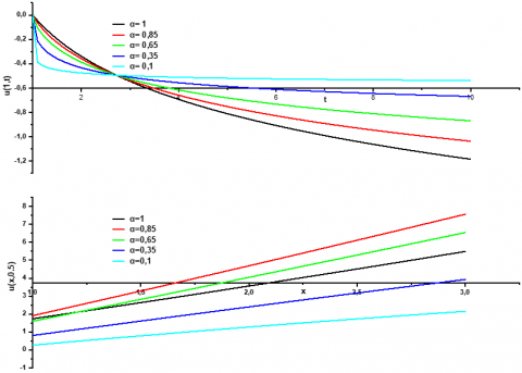
$\begin{gathered}U(x, t)=x\left(1-e^{\left(0.06 \ln \left(\frac{t}{a}\right)^\alpha\right)}\right)+\max \left(x-25 e^{-0.06}, 0\right) e^{\left(0.06 \ln \left(\frac{t}{a}\right)^\alpha\right)}\end{gathered}$ (40)
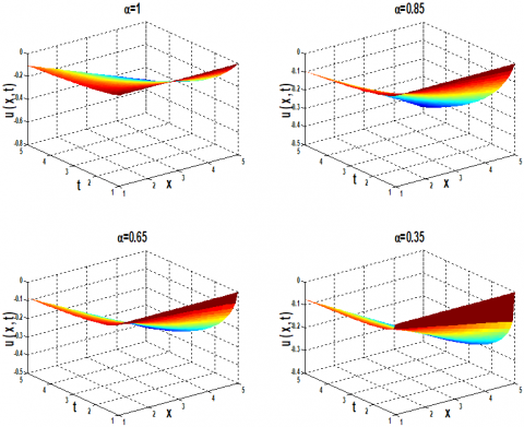
Solution plots of Eq. (40) is shown in Figure 3 for the different fractional parameter settings of α=0.85, 0.65, 0.35, 0.1 and 1, respectively. Financial pricing derivatives according to various fractional parameter settings (α=0.85, 0.65, 0.35, 0.1 and 1) are shown in Figure 4.
Figure 3. The graphs of Eq. (40) different value of parameter α with a=1, α=0.85, α=0.65, α=0.35, α=0.1
Figure 4. Surface shows the behavior of solution U(x, t) of application 2 using Eq. (40) with respect to t and x with α=1, α=0.85, α=0.65, α=0.35
In Table 2, the convergence of the series solution of Eq. (34) is demonstrated, which displays the numerical values of the solution produced by the homotopy perturbation approach and the precise solution Eq. (39) as well as the absolute errors with regard to certain specific varied values of t and $\alpha=1$. Additionally, numerical values for various values of $\alpha$ and $\varphi(\mathrm{t})=$ lnt are provided.
Table 2. Numerical values of the approximate and exact solutions Eq. (32) to Applications 1 for different values of t, and x=1, and α=1, α=0.85, α=0.65
|
t |
α=1, φ(t)=t |
||
|
$u_{exa}$ |
$u_{HPM}$ |
$err=\left|u_{exa}-u_{HPM}\right|$ |
|
|
1 |
-0,4946923 |
-0,4946923 |
0 |
|
1,1 |
-0,5458137 |
-0,5458137 |
0 |
|
1,2 |
-0,5972427 |
-0,5972427 |
0 |
|
1,3 |
-0,6489812 |
-0,6489812 |
0 |
|
1,4 |
-0,7010311 |
-0,7010311 |
0 |
|
1,5 |
-0,7533942 |
-0,7533942 |
0 |
|
1,6 |
-0,8060725 |
-0,8060725 |
0 |
|
1,7 |
-0,8590677 |
-0,8590677 |
0 |
|
1,8 |
-0,9123819 |
-0,9123819 |
0 |
|
1,9 |
-0,966017 |
-0,966017 |
0 |
|
2 |
-1,0199748 |
-1,0199748 |
0 |
|
2,1 |
-1,0742573 |
-1,0742573 |
0 |
|
2,2 |
-1,1288665 |
-1,1288665 |
0 |
|
2,3 |
-1,183804 |
-1,183804 |
0 |
|
2,4 |
-1,2390728 |
-1,2390728 |
0 |
|
2,5 |
-1,2946739 |
-1,2946739 |
0 |
|
2,6 |
-1,3506096 |
-1,3506096 |
0 |
|
2,7 |
-1,4068819 |
-1,4068819 |
0 |
|
2,8 |
-1,4634928 |
-1,4634928 |
0 |
|
2,9 |
-1,5204445 |
-1,5204445 |
0 |
|
3 |
-1,5777389 |
-1,5777389 |
0 |
|
t |
α=1, φ(t)=lnt |
α=0.85, φ(t)=lnt |
α=0.65, φ(t)=lnt |
|
$u_{HPM}$ |
$u_{HPM}$ |
$u_{HPM}$ |
|
|
1 |
0 |
0 |
0 |
|
1,1 |
-0,0458799 |
-0,0653548 |
-0,1048363 |
|
1,2 |
-0,0879947 |
-0,1137688 |
-0,1603625 |
|
1,3 |
-0,1269312 |
-0,1554157 |
-0,2037045 |
|
1,4 |
-0,1631479 |
-0,1924510 |
-0,2399895 |
|
1,5 |
-0,1970099 |
-0,2259771 |
-0,2714418 |
|
1,6 |
-0,2288128 |
-0,2566866 |
-0,2993003 |
|
1,7 |
-0,2587994 |
-0,2850611 |
-0,3243498 |
|
1,8 |
-0,2871717 |
-0,3114569 |
-0,3471284 |
|
1,9 |
-0,3140992 |
-0,3361478 |
-0,3680254 |
|
2 |
-0,3397260 |
-0,3593512 |
-0,3873336 |
|
2,1 |
-0,3641756 |
-0,3812429 |
-0,4052800 |
|
2,2 |
-0,3875543 |
-0,4019682 |
-0,4220449 |
|
2,3 |
-0,4099547 |
-0,4216484 |
-0,4377740 |
|
2,4 |
-0,4314576 |
-0,4403864 |
-0,4525872 |
|
2,5 |
-0,4521342 |
-0,4582700 |
-0,4665843 |
|
2,6 |
-0,4720476 |
-0,4753751 |
-0,4798495 |
|
2,7 |
-0,4912536 |
-0,4917678 |
-0,4924543 |
|
2,8 |
-0,5098022 |
-0,5075058 |
-0,5044604 |
|
2,9 |
-0,5277383 |
-0,5226400 |
-0,5159211 |
|
3 |
-0,5451022 |
-0,5372155 |
-0,5268826 |
In light of the findings presented in this research paper, the time-Fractional Black-Scholes European option pricing equation with boundary condition for a European option problem has been effectively solved using the homotopy perturbation technique and the $\varphi-$ Caputo Fractional derivative. Furthermore, this paper offers two instances that demonstrate the method's applicability and dependability under Caputo-Hadamard memory. Nonetheless, the results show that homotopy perturbation method is a strong and effective method for determining both precise and approximate answers to nonlinear fractional partial differential equations. The method's ability to reduce the amount of computing labour while retaining a high level of precision in the numerical result is crucial. Taking into account the Caputo-Hadamard fractional derivative, we visually portray the solutions to these issues using MATLAB to generate the graphs.
|
$\varphi$ |
growing function |
|
f |
be an integrable function |
|
T |
maturity date |
|
k |
the exercise price |
|
r(t) |
the risk-free interest rate |
|
σ(x,t) |
the volatility function of the underlying asset |
|
U(x,t) |
the price of a European call option at asset price x and at time t |
|
$\Gamma$(.) |
gamma function |
|
$\mathcal{J}_a^{\alpha ; \varphi}$ |
fractional integration operator |
|
${ }_t^C \mathcal{D}_a^{\alpha ; \varphi}$ |
Caputo fractional derivative |
|
${ }_t^C \mathcal{D}_a^{\alpha ; \varphi} u(x, t)$ |
derivative of u(x,t) in the Caputo sense |
|
R and N |
R and N denote linear and nonlinear differential operators |
|
g(x,t) |
stands for the source term |
|
$H_n(u)$ |
He’s polynomials |
|
a |
real number |
|
$\alpha$ |
order derivative |
[1] Black, F., Scholes, M. (1973). The pricing of options and corporate liabilities. Journal of Political Economy, 81(3): 637-654. https://doi.org/10.1142/9789814759588_0001
[2] Manale, J.M., Mahomed, F.M. (2000). A simple formula for valuing American and European call and put options. In Proceeding of the Hanno Rund Workshop on the Differential Equations.
[3] Gazizov, R.K., Ibragimov, N.H. (1998). Lie symmetry analysis of differential equations in finance. Nonlinear Dynamics, 17: 387-407. https://doi.org/10.1023/A:1008304132308
[4] Bohner, M., Zheng, Y. (2009). On analytical solutions of the Black-Scholes equation. Applied Mathematics Letters, 22(3): 309-313. https://doi.org/10.1016/j.aml.2008.04.002
[5] Company, R., Navarro, E., Pintos, J.R., Ponsoda, E. (2008). Numerical solution of linear and nonlinear Black-Scholes option pricing equations. Computers & Mathematics with Applications, 56(3): 813-821. https://doi.org/10.1016/j.camwa.2008.02.010
[6] Cen, Z., Le, A. (2011). A robust and accurate finite difference method for a generalized Black-Scholes equation. Journal of Computational and Applied Mathematics, 235(13): 3728-3733. https://doi.org/10.1016/j.cam.2011.01.018
[7] Company, R., Jódar, L., Pintos, J.R. (2009). A numerical method for European Option Pricing with transaction costs nonlinear equation. Mathematical and Computer Modelling, 50(5-6): 910-920. https://doi.org/10.1016/j.mcm.2009.05.019
[8] Fabião, F., Grossinho, M.D.R., Simões, O.A. (2009). Positive solutions of a Dirichlet problem for a stationary nonlinear Black-Scholes equation. Nonlinear Analysis: Theory, Methods & Applications, 71(10): 4624-4631. https://doi.org/10.1016/j.na.2009.03.026
[9] Amster, P., Averbuj, C.G., Mariani, M.C. (2002). Solutions to a stationary nonlinear Black-Scholes type equation. Journal of Mathematical Analysis and Applications, 276(1): 231-238. https://doi.org/10.1016/S0022-247X(02)00434-1
[10] Amster, P., Averbuj, C.G., Mariani, M.C. (2003). Stationary solutions for two nonlinear Black-Scholes type equations. Applied Numerical Mathematics, 47(3-4): 275-280. https://doi.org/10.1016/S0168-9274(03)00070-9
[11] Ankudinova, J., Ehrhardt, M. (2008). On the numerical solution of nonlinear Black-Scholes equations. Computers & Mathematics with Applications, 56(3): 799-812. https://doi.org/10.1016/j.camwa.2008.02.005
[12] Gülkaç, V. (2010). The homotopy perturbation method for the Black-Scholes equation. Journal of Statistical Computation and Simulation, 80(12): 1349-1354. https://doi.org/10.1080/00949650903074603
[13] Rasheed, M.A., Saeed, M.A. (2023). Numerical finite difference scheme for a two-dimensional time-fractional semilinear diffusion equation. Mathematical Modelling of Engineering Problems, 10(4): 1441-1449. https://doi.org/10.18280/mmep.100440
[14] Chandrasekaran, V., Rajendran, M., Nagarajan, R. (2025). Solving two-dimensional Black-Scholes equation by conformable Shehu homotopy analysis method. Mathematical Modelling of Engineering Problems, 12(2): 629-635. https://doi.org/10.18280/mmep.120226
[15] Warbhe, S., Gujarkar, V. (2023). Investigating thermal deflection in a finite hollow cylinder using quasi-static approach and space-time fractional heat conduction equation. International Journal of Heat and Technology, 41(6): 1605-1610. https://doi.org/10.18280/ijht.410623
[16] Oldham, K., Spanier, J. (1974). The Fractional Calculus Theory and Applications of Differentiation and Integration to Arbitrary Order. Elsevier.
[17] Miller, K.S. (1993). An Introduction to the Fractional Calculus and Fractional Differential Equations. John Willey & Sons.
[18] Podlubny, I. (1999). Fractional Differential Equations Calculus. New York: Academic Press.
[19] Kilbas, A.A., Srivastava, H.M., Trujillo, J.J. (2006). Theory and Applications of Fractional Differential Equations. Elsevier.
[20] Podlubny, I. (2001). Geometric and physical interpretation of fractional integration and fractional differentiation. arXiv preprint. https://doi.org/10.48550/arXiv.math/0110241
[21] Alqahtani, A.M., Mihoubi, H., Arioua, Y., Bouderah, B. (2025). Analytical solutions of time-fractional Navier–stokes equations employing homotopy perturbation–Laplace transform method. Fractal and Fractional, 9(1): 23. https://doi.org/10.3390/fractalfract9010023
[22] Mihoubi, H., Alqahtani, A.M., Arioua, Y., Bouderah, B., Tayebi, T. (2025). Homotopy perturbation ρ-Laplace transform approach for numerical simulation of fractional Navier-stokes equations. Contemporary Mathematics, 6(3): 2878-2906. https://doi.org/10.37256/cm.6320255978
[23] He, J.H. (2000). A coupling method of a homotopy technique and a perturbation technique for non-linear problems. International Journal of Non-Linear Mechanics, 35(1): 37-43. https://doi.org/10.1016/S0020-7462(98)00085-7
[24] He, J.H. (2006). Some asymptotic methods for strongly nonlinear equations. International Journal of Modern Physics B, 20(10): 1141-1199. https://doi.org/10.1142/S0217979206033796
[25] He, J.H. (2000). A new perturbation technique which is also valid for large parameters. Journal of Sound and Vibration, 5(229): 1257-1263. https://doi.org/10.1006/jsvi.1999.2509
[26] Yıldırım, A., Koçak, H. (2009). Homotopy perturbation method for solving the space-time fractional advection-dispersion equation. Advances in Water Resources, 32(12): 1711-1716. https://doi.org/10.1016/j.advwatres.2009.09.003
[27] Abdulaziz, O., Hashim, I., Ismail, E.S. (2009). Approximate analytical solution to fractional modified KdV equations. Mathematical and Computer Modelling, 49(1-2): 136-145. https://doi.org/10.1016/j.mcm.2008.01.005
[28] Yıldırım, A., Gülkanat, Y. (2010). Analytical approach to fractional Zakharov-Kuznetsov equations by He's homotopy perturbation method. Communications in Theoretical Physics, 53(6): 1005. https://doi.org/10.1088/0253-6102/53/6/02
[29] Khan, N.A., Ara, A., Mahmood, A. (2010). Approximate solution of time-fractional chemical engineering equations: A comparative study. International Journal of Chemical Reactor Engineering, 8(1): 2156. https://doi.org/10.2202/1542-6580.2156
[30] Wang, Q. (2007). Homotopy perturbation method for fractional KdV equation. Applied Mathematics and Computation, 190(2): 1795-1802. https://doi.org/10.1016/j.amc.2007.02.065
[31] Wang, Q. (2008). Homotopy perturbation method for fractional KdV-burgers equation. Chaos, Solitons & Fractals, 35(5): 843-850. https://doi.org/10.1016/j.chaos.2006.05.074
[32] Alqahtani, A.M. (2023). Solution of the generalized burgers equation using homotopy perturbation method with general fractional derivative. Symmetry, 15(3): 634. https://doi.org/10.3390/sym15030634
[33] Abdulaziz, O., Hashim, I., Ismail, E.S. (2009). Approximate analytical solution to fractional modified KdV equations. Mathematical and Computer Modelling, 49(1-2): 136-145. https://doi.org/10.1016/j.mcm.2008.01.005
[34] Omale, D., Gochhait, S. (2018). Analytical solution to the mathematical models of HIV/AIDS with control in a heterogeneous population using Homotopy Perturbation Method (HPM). Advances in Modelling and Analysis A, 55(1): 20-34. https://doi.org/10.18280/ama_a.550103
[35] Singh, J., Kumar, D., Kılıçman, A. (2013). Homotopy perturbation method for fractional gas dynamics equation using Sumudu transform. Abstract and Applied Analysis, 2013(1): 934060. https://doi.org/10.1155/2013/934060
[36] Ahmad, S., Ullah, A., Akgül, A., De la Sen, M. (2021). A novel homotopy perturbation method with applications to nonlinear fractional order KdV and burger equation with exponential-decay kernel. Journal of Function Spaces, 2021(1): 8770488. https://doi.org/10.1155/2021/8770488
[37] Jena, R.M., Chakraverty, S. (2019). Solving time-fractional Navier-Stokes equations using homotopy perturbation Elzaki transform. SN Applied Sciences, 1: 1-13. https://doi.org/10.1007/s42452-018-0016-9
[38] Ahmad, S., Ullah, A., Akgül, A., De la Sen, M. (2021). A novel Homotopy perturbation method with applications to nonlinear fractional order KdV and burger equation with exponential-decay kernel. Journal of Function Spaces, 2021(1): 8770488. https://doi.org/10.1155/2021/8770488
[39] Kheiri, H., Alipour, N., Dehghani, R. (2011). Homotopy analysis and homotopy pade methods for the modified Burgers-Korteweg-de Vries and the Newell-Whitehead equations. Mathematical Sciences, 5(1): 33-50.
[40] Bianchi, S. (2018). Fractional calculus and its applications. Risk and Decision Analysis, 7(1-2): 1-3. https://doi.org/10.3233/RDA-180138
[41] de Oliveira, E.C. (2019). Solved Exercises in Fractional Calculus. Berlin: Springer International Publishing. https://doi.org/10.1007/978-3-030-20524-9
[42] Almeida, R. (2017). A Caputo fractional derivative of a function with respect to another function. Communications in Nonlinear Science and Numerical Simulation, 44: 460-481. https://doi.org/10.1016/j.cnsns.2016.09.006
[43] Samko, S.G. (1993). AA Kilbas and 0.1. Marichev. Fractional Intearals and Derivatives: Theorv and Agglications.
[44] Jarad, F., Abdeljawad, T., Baleanu, D. (2012). Caputo-type modification of the Hadamard fractional derivatives. Advances in Difference Equations, 2012: 1-8. https://doi.org/10.1186/1687-1847-2012-142
[45] Mittag-Leffler, G.M. (1903). Sur la nouvelle fonction Eα (x). CR Academy of Sciences, 137(2): 554-558.
[46] West, B.J., Bologna, M., Grigolini, P. (2003). Physics of Fractal Operators. New York: Springer. https://doi.org/10.1007/978-0-387-21746-8
[47] He, J.H. (1999). Homotopy perturbation technique. Computer Methods in Applied Mechanics and Engineering, 178(3-4): 257-262. https://doi.org/10.1016/S0045-7825(99)00018-3
[48] Ghorbani, A. (2009). Beyond Adomian polynomials: He polynomials. Chaos, Solitons & Fractals, 39(3): 1486-1492. https://doi.org/10.1016/j.chaos.2007.06.034
[49] Edeki, S.O., Ugbebor, O.O., Owoloko, E.A. (2015). Analytical solutions of the Black-Scholes pricing model for European option valuation via a projected differential transformation method. Entropy, 17(11): 7510-7521. https://doi.org/10.3390/e17117510
[50] Saratha, S.R., Sai Sundara Krishnan, G., Bagyalakshmi, M., Lim, C.P. (2020). Solving Black-Scholes equations using fractional generalized homotopy analysis method. Computational and Applied Mathematics, 39: 1-35. https://doi.org/10.1007/s40314-020-01306-4