Hiba H. Abdullah![]() | Nihad S. Khalaf Aljboori
| Nihad S. Khalaf Aljboori![]() | Nooruldeen A. Noori*
| Nooruldeen A. Noori*![]()
© 2025 The authors. This article is published by IIETA and is licensed under the CC BY 4.0 license (http://creativecommons.org/licenses/by/4.0/).
OPEN ACCESS
This study aims to analyze the stability of conditional variance and evaluate the productive performance of NAGARCH models when applied to natural gas future price. The research relied on the local linear approximation technique to transform nonlinear models into linear differential equations, with hybrid model combining NAGARCH and ARMA applied to improve the forecast. Monthly historical data of natural gas futures (May 1990- February 2022) were used to evaluate the performance. The results showed that the NAGARCH(1,1) model was the most stable according to the AIC, and BIC criteria, and was used with ARIMA(1,0,1) to create a hybrid model. However, the hybrid model suffered from poor predictive performance when comparing actual values with forecasts. The study highlights the importance of incorporating advanced methods to improve forecasts and reduce instability caused by price fluctuations.
ARCH, GARCH, NAGARCH, Box-Jenkins methodology, stability conditional variance, local linearization method, limit cycle, heteroscedastic
The stochastic process is described as second order stationary that is meant a variance and mean in the process are fixed is not reliant on time , the majority of significant condition for random error all the time model series ought to be the white noise process with constant variance and zero mean and uncorrelated. This model was discussed by a number of researchers and suggested some nonlinear time series model referred to as autoregressive conditional, heteroscedastic avoidance volatility in data, that causes dependency mean and variance on time t. The basic model suggestion in 1982 by R. Engle abbreviated as ARCH [1].
Quite a few researchers have studied and extended the stability of these extension ARCH and GARCH models. Glosten et al. [2] proposed GJR-GARCH.
Non-linear Asymmetric Generalized Autoregressive Conditional Heteroscedasticity Variance model in 1992 which was short (NAGARCH model) proposed the NAGARCH model as an expansion of GARCH model [3].
Motivation for a study:
The research aims to develop and analyze the stability of the NAGARCH model to determine the optimal conditions for stability and apply the NAGARCH model to natural gas price data to verify the predictive performance in addition to integrating the NAGARCH model with ARIMA to create a hybrid model and analyze its performance compared to individual models.
The importance of the research is in providing accurate tools for analyzing natural gas price fluctuations, which enables decision-makers in the energy and finance sectors to predict fluctuations and make informed decisions. It also contributes to bridging the research gap by expanding the uses of NAGARCH models and analyzing their stability, as research combines NAGARCH model with ARIMA model, opening new horizons in hybrid models for analyzing time data. NAGARCH was chosen compared to other models because: dealing with asymmetry: it’s characterized by its ability to deal with the effects of different shocks on the conditional variance, provides more advanced techniques for analyzing the dynamics of volatile markets, and previous studies have proven its effectiveness in analyzing commodities and markets that change in a manner similar to natural gas.
NAGARCH(Q,P) models will a new stability conditions by using the local linear approximation technique and converting the nonlinear model into a difference equation with fixed coefficients proposed by Ozaki [4] when he detect the exponential autoregressive model's stability condition (EXPAR). Ali and Mohammad [5] found stability conditions of limit cycle for Gompertz Autoregressive model, Mohammad and Mudhir [6] found the stability of the EGARCH model, stability of GJR-GARCH model by Noori and Mohammad [7], stability conditions for a nonlinear time series model [8], N-SIR by Hussien and Azher [9], and stability exponential double autoregressive model [10].
This study including three sections: Section 1 including introduction, Section 2 including some primaries and theorems with its proving to find a stability of NAGARCH model, while Section 3 including application to apply the conditions which was finds in Section 2.
The discrete dynamical systems outlined by the system can be signified as a nonlinear time series model in discrete time.
$x_t=f\left(x_{t-1}, x_{t-2}, \ldots, x_{t-p}, e_t\right)$ (1)
where, f: nonlinear function, $e_t$: white noise process $\left(e_t \sim i i d N\left(0, \psi_e^2\right)\right)$.
The Autoregressive Conditional Heteroscedasticity Variance model shortly (ARCH model) that Robert Engle proposed with the formulation:
$x_t=\psi_t e_t$ where $e_t \sim \operatorname{iid} N(0,1)$
$\psi_t^2=w+\sum_{i=1}^K \eta_i x_{t-i}^2$ (2)
where, $w, \sum_{i=1}^Q \eta_i$: parameters of model. $\psi_t^2$: conditional variance [11].
A martingale difference that is implemented in this model
$E\left(x_{t+1}^2 / \Upsilon_t\right)=\psi_t^2$ (3)
where, $\Upsilon_t$ is filter of a random variable $\left(x_{t-1}, x_{t-2}, \ldots, x_{t-K}\right)$ [12], by using dynamical system to convey (2) as:
$\psi_t^2=f\left(w, \psi_{t-1}^2, \psi_{t-2}^2, \ldots, \psi_{t-K}^2\right)$ (4)
The local linearization approach (LLA) focuses on the stability of a non-zero fixed point of the original dynamic system in order to investigate and converge a nonlinear dynamical system to a linear dynamical system. A non-zero singular point $\zeta$ of a function $f$. If their vicinity is devoid of any other fixed points. The necessary and sufficient condition for $\zeta$ is met [13]:
$\zeta=f(\zeta)$ (5)
This method combines the effect of slightly disturbing a non-zero singular point ζ in its vicinity with a sufficiently tiny radius $\zeta_t$ to ensure that $\zeta_t^n \rightarrow 0$ for $\mathrm{n} \geq 2$. The impact of this little discomfort is caused by substituting $\zeta+\zeta_{t-i}$ for $1 \leq i \leq K$ in state $\psi_t-i^2$ hence, we use the following variational equation [14]:
$\psi_{t-i}^2=\zeta_{t-i}+\zeta$ for $1 \leq i \leq K$ (6)
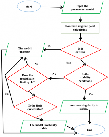
Once this variation equation comes in Eq. (4), we can next add a linear difference equation of order K in terms of $\zeta_t, \zeta_{t-1}, \zeta_{t-2}, \ldots, \zeta_{t-K}$. Using the roots of its characteristic equation, we can debate the stability of the linear difference equation. The following diagram represents the flowchart for studying the stability of nonlinear models of time series.
Box-Jenkins methodology was developed by Box and Jenkins in 1970 with the aim of finding the most appropriate model and using it for forecasting, although this methodology was mentioned in many sources and divided into five or six stages, but we can summarize this method as follows: Model Identification, Parameters Estimation, Diagnostic Checking and Forecast [15].
Lemma 2.1 [16]
Let $\eta_1, \eta_2, \ldots, \eta_r \in R^{+}$, the subsequent polynomial:
$P(\omega)=1-\sum_{i=1}^r \eta_i \omega^i$
has no roots within or on the unit circle iff $P(\omega)>1$.
In 1986 suggested GARCH(Q,P) has the formula below [17]:
$x_t=\psi_t e_t$
$\psi_t^2=w+\sum_{i=1}^Q \eta_i x_{t-i}^2+\sum_{j=1}^P \delta_j \psi_{t-j}^2$ (7)
Figure 1 shows the flowchart of the stability of nonlinear models of time series in dynamic method.
Figure 1. Flowchart for the study of the stability of nonlinear models of time series
Numerous models in which amplification is used and intended of the GARCH model. But NAGARCH’s model possesses the form:
$x_t=\psi_t e_t$
$\psi_t^2=w+\sum_{i=1}^Q \eta_i\left(x_{t-i}-\gamma_i \psi_{t-i}\right)^2+\sum_{j=1}^P \delta_j \psi_{t-j}^2$ (8)
$\begin{gathered}\psi_t^2=w+\sum_{i=1}^Q \eta_i x_{t-i}^2-2 \eta_i \gamma_i x_{t-i} \psi_{t-i}+\gamma_i^2 \psi_{t-i}^2 +\sum_{j=1}^P \delta_j \psi_{t-j}^2\end{gathered}$
$\begin{gathered}\psi_t^2=w+\sum_{i=1}^Q \eta_i\left(x_{t-i}^2-2 \gamma_i \psi_{t-i}^2 e_{t-i}+\gamma_i^2 \psi_{t-i}^2\right)+\sum_{j=1}^P \delta_j \psi_{t-j}^2\end{gathered}$ (9)
Iff the NAGARCH process becomes stationary
$\left[\sum_{i=1}^Q \eta_i\left(1+\gamma_i^2\right)+\sum_{j=1}^P \delta_j\right]<1$ (10)
In this case the variance is $\psi_x^2=E\left(x_t^2 / Y_t\right)=E\left(x_{t-i}^2 / Y_t\right)$ for $i=1,2, \ldots, Q$, according to the supposition that the stochastic process of squares $\left\{x_t^2\right\}$ is stationary.
Next, on both sides of the equation, the conditional expectation has to be included in the filter $Y_t$ that we derive Eq. (9).
$\begin{gathered}\mathrm{E}\left(\psi_t^2 / \Upsilon_t\right) =E\left(w / \Upsilon_t\right)+\sum_{i=1}^Q \eta_i \mathrm{E}\left(\left(x_{t-i}^2-2 \gamma_i \psi_{t-i}^2 e_{t-i}+\gamma_i^2 \psi_{t-i}^2\right) / \Upsilon_t\right) +\sum_{j=1}^P \delta_j \mathrm{E}\left(\psi_{t-j}^2 / \Upsilon_t\right)\end{gathered}$
$\psi_x^2=w+\sum_{i=1}^Q \eta_i\left(1+\gamma_i^2\right) \psi_x^2+\sum_{j=1}^P \delta_j \psi_x^2$ (11)
So the unconditional variance of the model in Eq. (4) is provided by
$\psi_x^2=\frac{w}{1-\left[\sum_{i=1}^Q \eta_i\left(1+\gamma_i^2\right)+\sum_{j=1}^P \delta_j\right]}$ (12)
Of the unconditional variance $\psi_x^2$ exists if
$\left[\sum_{i=1}^Q \eta_i\left(1+\gamma_i^2\right)+\sum_{j=1}^P \delta_j\right]<1$
Subsequently, as per reference [18], the NAGARCH model's stationarity required that the conditional variance $\psi_t^2$ converges the unconditional variance $\psi_x^2$. By using LLA $x_t=\psi_t e_t$, as long as:
$\begin{gathered}E\left(x_t\right)=E\left(\psi_t e_t\right)=E\left(e_t\right) \cdot E\left(\psi_t\right)=E\left(\psi_t\right) \cdot 0=0 \\{Var}\left(x_t\right)=\mathrm{E}\left(x_t^2\right)=\mathrm{E}\left(e_t^2 \cdot \psi_t^2\right)=\psi_t^2 \cdot \mathrm{E}\left(e_t^2\right)=\psi_t^2 \cdot 1=\psi_t^2\end{gathered}$
We ensure that it is occupied a conditional expectation and paid attention to the filtering $\Upsilon_{t-i}$ for $i=1,2, \ldots, Q$ on both sides of the model Eq. (9).
$\begin{gathered}\mathrm{E}\left(\psi_t^2 / \Upsilon_t\right)=E\left(w / \Upsilon_t\right) \\ +\sum_{i=1}^Q \eta_i \mathrm{E}\left(\left(x_{t-i}^2-2 \gamma_i \psi_{t-i}^2 e_{t-i}+\gamma_i^2 \psi_{t-i}^2\right) / \Upsilon_{t-i}\right) \\ +\sum_{j=1}^P \delta_j \mathrm{E}\left(\psi_{t-j}^2 / \Upsilon_{t-j}\right)\end{gathered}$
$\psi_t^2=w+\sum_{i=1}^Q \eta_i \cdot \psi_{t-i}^2+\sum_{i=1}^Q \eta_i \cdot \gamma_i^2 \cdot \psi_{t-i}^2+\sum_{j=1}^P \delta_j \cdot \psi_{t-j}^2$
$\begin{gathered}\psi_t^2=w+\sum_{i=1}^Q \eta_i \psi_{t-i}^2+\sum_{i=1}^Q \eta_i \cdot \gamma_i^2 \cdot \psi_{t-i}^2 +\sum_{j=1}^P \delta_j \psi_{t-j}^2\end{gathered}$ (13)
By put $\psi_t^2=\psi_{t-1}^2=\psi_{t-2}^2=\cdots=\psi_{t-Q}^2=\psi_{t-P}^2=\zeta$ to get a fixed point
$\zeta=w+\left[\sum_{i=1}^Q \eta_i\left(1+\gamma_i^2\right)+\sum_{j=1}^P \delta_j\right] \zeta$ (14)
$\therefore \zeta=\frac{w}{\left[1-\sum_{i=1}^Q \eta_i\left(1+\gamma_i^2\right)-\sum_{j=1}^P \delta_j\right]}$
Then the non-zero singular point satisfies the condition in Eq. (5) of the NAGARCH model is $\psi_x^2$ (unconditional variance).
Let $r=\max (Q, P)$ then when $Q>P$ put $\eta_r\left(1+\gamma_r^2\right)=0$ for $r=P, P+1, \ldots, Q-1$ if else put $\delta_r=0$ for $r=Q, Q+$ $1, \ldots, P-1$ then NAGARCH becomes:
$\begin{gathered}\psi_t^2=w+\sum_{i=1}^Q \eta_i\left(x_{t-i}^2-2 \gamma_i \psi_{t-i}^2 e_{t-i}+\gamma_i^2 \psi_{t-i}^2\right) +\sum_{j=1}^P \delta_j \psi_{t-j}^2\end{gathered}$
Of the unconditional variance
$\zeta=\psi_x^2=\frac{w}{\left[1-\sum_{i=1}^r\left[\eta_i\left(1+\gamma_i^2\right)+\delta_i\right]\right.}$ (15)
Proposition 2.1:
The NAGARCH model's non-zero singular point is stable iff
$\left[\sum_{i=1}^r \eta_i\left(1+\gamma_i^2\right)+\delta_i\right]<1$
Proof:
In the vicinity of a non-zero singular point with a radius of $\zeta_t$ that is sufficiently small to cause $\zeta_t^n \rightarrow 0$ for $n \geq 2$, we substitute $\zeta+\zeta_{t-i}$ in state $\psi_{t-i}^2$ for $i=0,1, \ldots, r$ Eq. (13) gives:
$\zeta+\zeta_t=w+\sum_{i=1}^r\left(\eta_i\left(1+\gamma_i^2\right)+\delta_i\right)\left(\zeta+\zeta_{t-i}\right)$
$\begin{aligned} \zeta+\zeta_t & =w+\sum_{i=1}^r\left(\eta_i\left(1+\gamma_i^2\right)+\delta_i\right) \zeta +\sum_{i=1}^r\left(\eta_i\left(1+\gamma_i^2\right)+\delta_i\right) \zeta_{t-i}\end{aligned}$
$\begin{gathered}\zeta\left[1-\sum_{i=1}^r\left(\eta_i\left(1+\gamma_i^2\right)+\delta_i\right)\right]-w+\zeta_t =\sum_{i=1}^r\left(\eta_i\left(1+\gamma_i^2\right)+\delta_i\right) \zeta_{t-i}\end{gathered}$
But $\zeta\left[1-\sum_{i=1}^r\left(\eta_i\left(1+\gamma_i^2\right)+\delta_i\right)\right]=w$ from Eq. (15)
$\zeta_t=\sum_{i=1}^r\left(\eta_i\left(1+\gamma_i^2\right)+\delta_i\right) \zeta_{t-i}$ (16)
Eq. (16) is a fixed coefficient The characteristic equation and the linear difference Eq. (16), on the other hand, can be expressed as
$\lambda^{\mathrm{r}}-\sum_{i=1}^r\left(\eta_i\left(1+\gamma_i^2\right)+\delta_i\right) \lambda^{\mathrm{r}-\mathrm{i}}=0$ (17)
The non-zero singular point is stable, i.e., $\left|\varphi_i\right|<1$ for $i.=0,1,2, ... ,r$. Where $\varphi_i$ is the root of characteristic equation for Eq. (17). From Eq. (17)
$\lambda^r\left(1-\sum_{i=1}^r\left(\eta_i\left(1+\gamma_i^2\right)+\delta_i\right) \lambda^{-\mathrm{i}}\right)=0$
$\begin{gathered}P\left(\frac{1}{\lambda}\right)=1-\sum_{i=1}^r\left(\eta_i\left(1+\gamma_i^2\right)+\delta_i\right)\left(\frac{1}{\lambda}\right)^i=0 \text { (since } \lambda^r \neq 0 \text { ) }\end{gathered}$ (18)
then by Lemma (2.1) we get: inside and on the unit cycle, the polynomial (18) has no roots if and only if $P\left(\frac{1}{\lambda}\right)>0$
$\begin{aligned} & \because\left|\frac{1}{\lambda_i}\right|>1 \text { for } i .=0,1,2, \ldots, r \\ & \therefore\left|\lambda_i\right|<1 \text { for } i .=0,1,2, \ldots, r\end{aligned}$
and on account of $P(1) .>0$ then
$\left[1-\sum_{i=1}^r\left(\eta_i\left(1+\gamma_i^2\right)+\delta_i\right)\right]>0$
which implies that $\sum_{i=1}^r\left(\eta_i\left(1+\gamma_i^2\right)+\delta_i\right)<1$. $\blacksquare$
Proposition 2.2:
If the NAGARCH(1,1) model possesses a limit cycle of period $k>0$ then this limit cycle is orbitally stable if:
$\left|\prod_{j=1}^k\left[\frac{1 \psi_{t+j-1}}{\psi_{t+j}}\right]\right|<\frac{1}{\left|\eta_1\left(1+\gamma_1^2\right)+\delta_1\right|^k}$
Proof:
Assume the model has a limit cycle with period k, i.e.,
$\psi_t^2, \psi_{t+1}^2, \psi_{t+2}^2, \ldots, \psi_{t+k}^2=\psi_t^2$
Each point in a limit cycle is in the neighborhood of another with small radius enough $\zeta_t$ such that $\zeta_t^n \rightarrow 0$ for $n \geq 2$ placed $\psi_t=\psi_t+\zeta_t, \psi_{t-1}=\psi_{t-1}+\zeta_{t-1}$.
The NAGARCH’s model is given by:
$\psi_t^2=w+\eta_1\left(x_{t-1}^2-2 \gamma_1 \psi_{t-1}^2 e_{t-1}+\gamma_1^2 \psi_{t-1}^2\right)+\delta_1 \psi_{t-1}^2$
By combining the conditional expectations of both parties in terms of filters $Y_t, Y_{t-1}$, we get:
$\begin{gathered}\psi_t^2=w+\eta_1\left(1+\gamma_1^2\right) \psi_{t-1}^2+\delta_1 \psi_{t-1}^2 \\ \psi_t^2=w+\left(\eta_1\left(1+\gamma_1^2\right)+\delta_1\right) \psi_{t-1}^2 \\ \left(\psi_t+\zeta_t\right)^2=w+\left(\eta_1\left(1+\gamma_1^2\right)+\delta_1\right)\left(\psi_{t-1}+\zeta_{t-1}\right)^2 \\ \psi_t^2+\zeta_t^2+2 \psi_t \zeta_t=w+\left(\eta_1\left(1+\gamma_1^2\right)+\delta_1\right)\left(\psi_{t-1}^2+\zeta_{t-1}^2\right. \left.+2 \psi_{t-1} \zeta_{t-1}\right)\end{gathered}$
By our assuming $\zeta_t^2, \zeta_{t-1}^2 \rightarrow 0$
$\begin{aligned} & \psi_t^2+2 \psi_t \zeta_t=w+( \left.\eta_1\left(1+\gamma_1^2\right)+\delta_1\right)\left(\psi_{t-1}^2+2 \psi_{t-1} \zeta_{t-1}\right) \\ & \psi_t^2+2 \psi_t \zeta_t=w+\left(\eta_1\left(1+\gamma_1^2\right)+\delta_1\right)\left(\psi_t^2+2 \psi_{t-1} \zeta_{t-1}\right) \\ & \psi_t^2+2 \psi_t \zeta_t=w+\left(\eta_1\left(1+\gamma_1^2\right)+\delta_1\right) \psi_t^2 +\left(\eta_1\left(1+\gamma_1^2\right)+\delta_1\right) 2 \psi_{t-1} \zeta_{t-1} \\ & \psi_t^2\left[1-\left(\eta_1\left(1+\gamma_1^2\right)+\delta_1\right)\right]-w+2 \psi_t \zeta_t =\left(\eta_1\left(1+\gamma_1^2\right)+\delta_1\right) 2 \psi_{t-1} \zeta_{t-1}\end{aligned}$
But, $w=\psi_t^2\left[1-\left(\eta_1\left(1+\gamma_1^2\right)+\delta_1\right)\right]$, we get:
$2 \psi_t \zeta_t=\left(\eta_1\left(1+\gamma_1^2\right)+\delta_1\right) 2 \psi_{t-1} \zeta_{t-1}$
$\zeta_t=\frac{\left(\eta_1\left(1+\gamma_1^2\right)+\delta_1\right)}{\psi_t} \psi_{t-1} \zeta_{t-1}$ (19)
From Eq. (19) and after $k$ times, we get:
$\zeta_t=\left[\frac{\left(\eta_1\left(1+\gamma_1^2\right)+\delta_1\right)}{\psi_{t-k}} 1 \psi_{t-k-1}\right] \zeta_{t-k}$
But
$\begin{gathered}\zeta_{t-k}=\left[\frac{\left(\eta_1\left(1+\gamma_1^2\right)+\delta_1\right)}{\psi_{t-k}} 1 \psi_{t-(k+1)}\right] \zeta_{t-(k+1)} \\ \zeta_{t+k}=\prod_{j=1}^k\left[\frac{\left(\eta_1\left(1+\gamma_1^2\right)+\delta_1\right)}{\psi_{t+j}} \psi_{t+j-11}\right] \zeta_t\end{gathered}$
$\therefore \frac{\zeta_{t+k}}{\zeta_t}=\prod_{j=1}^k\left[\frac{\left(\eta_1\left(1+\gamma_1^2\right)+\delta_1\right)}{\psi_{t+j}} \psi_{t+j-11}\right]$
The Eq. (19) is a linear difference equation with a variable coefficient of the first order and its solution is a very difficult process but what interests us is that solution to the difference equation converge to zero as $t$ gets larger $t \rightarrow \infty$, this solution is convergence, then this limit cycle is orbitally stable. This convergence only takes place if and only if the following condition is holding:
$\left|\frac{\zeta_{t+k}}{\zeta_t}\right|<1$ (20)
From condition (20) and Eq. (19) the NAGARCH (1,1) is orbitally stable if:
$\begin{gathered}\left|\frac{\zeta_{t+k}}{\zeta_t}\right|=\left|\prod_{j=1}^k\left[\frac{\left(\eta_1\left(1+\gamma_1^2\right)+\delta_1\right)}{\psi_{t+j}} \psi_{t+j-11}\right]\right|<1 \\ \left|\eta_1\left(1+\gamma_1^2\right)+\delta_1\right|^k\left|\prod_{j=1}^k\left[\frac{\psi_{t+j-11}}{\psi_{t+j 1}}\right]\right|<1 \\ \left|\prod_{j=1}^k\left[\frac{\psi_{t+j-1}}{\psi_{t+j}}\right]\right|<\frac{1}{\left|\eta_1\left(1+\gamma_1^2\right)+\delta_1\right|^k} . \blacksquare \end{gathered}$
The NAGARCH model has no limit cycle.
3.1 Data descriptions
The data used in our study represents monthly mean of historical data natural gas contracts from: MAY.1990-FEB.2022 by 381 views. Data availability the data used to support the finding of this study is available on the following website https://sa.investing.com/commodities/natural-gas-historical-data.
3.2 Modeling and building the NAGARCH model
The modeling and programming process NAGARCH’s model is applied to the data series. We note and verify that the predicted conditional variance value approaches the value of the unconditional variance. Parameters estimation by AIC, and BIC criteria, and then predict the value of the conditional variance, it is worth noting that to study the GARCH family models, we will follow the Box-Jenkins methodology, provided that the heterogeneity is detected; Because the architecture of GARCH models is very close in syntax to ARMA models.
Analysis Steps:
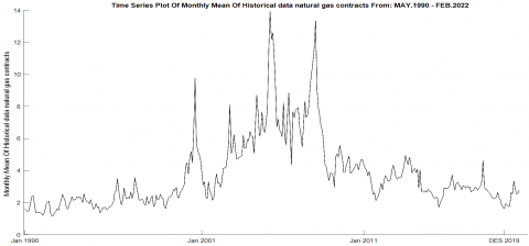
(1) We enter the data into the program used to create the data sequence, where the Figure 2 is represented by monthly mean of historical data natural gas contracts.
Figure 2. Represented monthly mean of historical data natural gas contracts
It is noticeable when the time series is drawn that it follows irregular components, that is, the series of result of unexpected and irregular effects, and also does not repeat a specific pattern, the diagram helps visualize the process of identifying fixed points and checking their stability. Then follows the step of drawing the time series to convert the series to a return series and we do this conversion by using the mathematical formula.
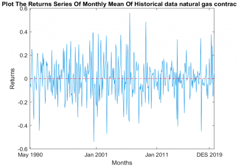
$r_t=\log \left(\frac{x_t}{x_{t-1}}\right)=\log x_t-\log x_{t-1}$
where, $r_t$ is returns series and $x_t, x_{t-1}$ are observation at $t, t-1$ respectively. Figure 3 expresses the series of returns.
Figure 3. The series of returns
Figure 3 shows the general trends and fluctuations in natural gas prices over the study period. The series shows random fluctuations and no clear seasonal pattern.
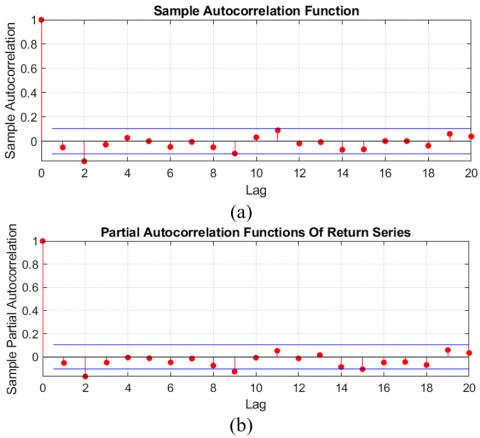
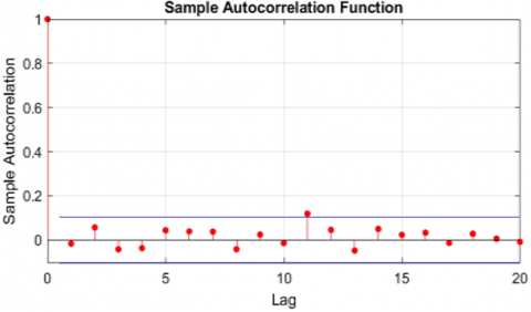
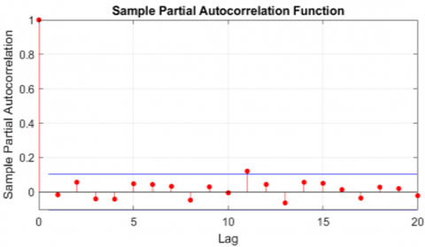
Although the time series possessed stability, it still suffers from some correlations that we have to remove. This is evident by drawing the ACF and PACF functions as in Figure 4 where, the correlations appear outside the confidence intervals specified $\pm \frac{1.96}{\sqrt{n}}$ where $n$ is the sample size [24].
Figure 4. ACF and PACF functions for the time series
We can notice from the previous figure that there are a number of lags outside the boundaries of the confidence interval that need to be addressed before starting the modeling and forecasting process [25].
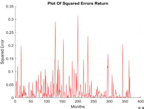
(2) To find out whether there is an effect of variance heterogeneity by finding the error-squared series of a return’s series out of the rapport $e_t=\left(r_t-\bar{r}_t\right)^2$, where $\bar{r}_t$ is the mean of the returns.
Figure 5. The error-squared series of the return’s series
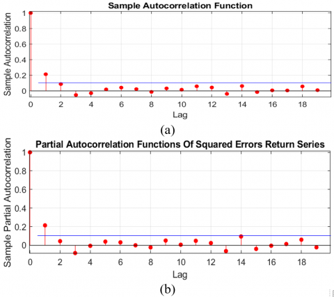
Figure 6. ACF and PACF functions for the error-squared series of the return’s series
Figure 5 shows the squared errors of the time series of returns. The series exhibits non-stationary variance, indicating heteroscedasticity, Figure 6 shows values outside the confidence intervals, indicating conditional heteroscedasticity, we notice that some values still fall outside the confidence interval in the ACF and PACF functions at the time differences (Lags) for $k=1,2$.
(3) To detect attacks in return series, we use the Ljung-Box test to measure the effect of heteroscedasticity where the “Table 1” represents the test results.
From Table 1, it is noted that at most lags, the p-value is less than 0.05, indicating that there is autocorrelation in the series. This means that the data needs further processing to remove autocorrelation before modeling.
Table 1. Results of the Ljung-Box test for return series
|
Lags |
h-value |
p-value |
Q-Test |
Critical Value |
|
Lag1 |
0 |
0.3189 |
0.9936 |
3.8415 |
|
Lag2 |
1 |
0.0037 |
11.2222 |
5.9915 |
|
Lag3 |
1 |
0.0092 |
11.5264 |
7.8147 |
|
Lag4 |
1 |
0.0189 |
11.8049 |
9.4877 |
|
Lag5 |
1 |
0.0376 |
12.6394 |
11.0705 |
|
Lag6 |
1 |
0.0491 |
12.6522 |
12.5916 |
|
Lag7 |
0 |
0.0810 |
13.6109 |
14.0671 |
|
Lag8 |
0 |
0.0925 |
17.5530 |
15.5073 |
|
Lag9 |
1 |
0.0407 |
17.9364 |
16.9190 |
|
Lag10 |
0 |
0.0560 |
20.9780 |
18.3070 |
|
Lag11 |
1 |
0.0336 |
21.1155 |
19.6751 |
|
Lag12 |
1 |
0.0487 |
21.1380 |
21.0261 |
|
Lag13 |
0 |
0.0702 |
23.0555 |
22.3620 |
|
Lag14 |
0 |
0.0594 |
24.8331 |
23.6848 |
|
Lag15 |
0 |
0.0522 |
24.8334 |
24.9958 |
|
Lag16 |
0 |
0.0728 |
24.8335 |
26.2962 |
|
Lag17 |
0 |
0.0985 |
25.3659 |
27.5871 |
|
Lag18 |
0 |
0.1152 |
26.7629 |
28.8693 |
|
Lag19 |
0 |
0.1103 |
27.3684 |
30.1435 |
|
Lag20 |
0 |
0.1252 |
24.7535 |
31.4104 |
(4) Now we fit parameters estimation for the model in order to choose the best rank for the model, we will use AIC, CAIC and BIC information criteria and calculate the values. Where Table 2 gives the values of AIC, and BIC criteria for different ranks of the NAGARCH’s model.
Table 2. The values of AIC, CAIC and BIC criteria for different ranks of the NAGARCH
|
NAGARCH(P,Q) |
AIC |
BIC |
|
NAGARCH(1,1) |
-340.9731 |
-325.3299 |
|
NAGARCH(1,2) |
-340.1856 |
-316.7208 |
|
NAGARCH(1,3) |
-337.7223 |
-306.4359 |
|
NAGARCH(1,4) |
-333.7223 |
-294.6144 |
|
NAGARCH(2,1) |
-338.9731 |
-319.4191 |
|
NAGARCH(2,2) |
-338.1856 |
-310.8100 |
|
NAGARCH(2,3) |
-335.7223 |
-300.5251 |
|
NAGARCH(2,4) |
-331.7223 |
-288.7036 |
|
NAGARCH(3,1) |
-336.9731 |
-313.5083 |
|
NAGARCH(3,2) |
-336.1856 |
-304.8992 |
|
NAGARCH(3,3) |
-333.7223 |
-294.6144 |
|
NAGARCH(3,4) |
-329.7223 |
-282.7928 |
Table 2 shows a comparison between the performance of different NAGARCH models based on AIC and BIC criteria. From this, we get that the best model is NAGARCH(1,1), as it achieved the lowest value for both AIC and BIC. Also, increasing the model order (P,Q) led to a decrease in the quality of the model due to the increase in complexity, so the model formula is $x_t=\psi_t e_t$ where $e_t \sim iid\ N(0,1)$
$\begin{gathered}\psi_t^2=0.016519 +0.043359\left(x_{t-i}-0.37924 \psi_{t-i}\right)^2-0.18201 \psi_{t-j}^2\end{gathered}$ (21)
And by implementation When we examine the model's stability conditions, we see that it is stable according to the condition in Eq. (10), then:
$\begin{aligned} \eta_1\left(1+\gamma_1^2\right)+\delta_1 & =0.043359\left[1+(0.37924)^2\right]-0.18201 =-0.1324149795<1\end{aligned}$
The value of the NAGARCH model's unconditional variance is given in Eq. (15) as follows:
$\psi^2=0.0247$
(5) Now checking the adequacy of the model this stage is to check the suitability of the chosen model in order to verify the adequacy of the NAGARCH(1,1) model in interpreting the data used in calculating future predictions, but the standard series must be checked. Perform a Ljung-Box test and plot the ACF and PACF functions, but on the residual series.
From the Table 3, it's noted that most of the p-values are high 0.05, indicating that the model explains the time series well and there is no longer autocorrelation.
Table 3. Results of the Ljung-Box test for the standard residuals series
|
Lags |
h-value |
p-value |
Q-Test |
Critical Value |
|
Lag1 |
0 |
0.7523 |
0.0996 |
3.8415 |
|
Lag2 |
0 |
0.5172 |
1.3186 |
5.9915 |
|
Lag3 |
0 |
0.5779 |
1.9736 |
7.8147 |
|
Lag4 |
0 |
0.6487 |
2.4776 |
9.4877 |
|
Lag5 |
0 |
0.6691 |
3.2009 |
11.0705 |
|
Lag6 |
0 |
0.7081 |
3.7676 |
12.5916 |
|
Lag7 |
0 |
0.7442 |
4.3036 |
14.0671 |
|
Lag8 |
0 |
0.7613 |
4.9647 |
15.5073 |
|
Lag9 |
0 |
0.8173 |
5.1912 |
16.9190 |
|
Lag10 |
0 |
0.8730 |
5.2621 |
18.3070 |
|
Lag11 |
0 |
0.4698 |
10.6879 |
19.6751 |
|
Lag12 |
0 |
0.4871 |
11.4937 |
21.0261 |
|
Lag13 |
0 |
0.4973 |
12.3728 |
22.3620 |
|
Lag14 |
0 |
0.5001 |
13.3377 |
23.6848 |
|
Lag15 |
0 |
0.5604 |
13.5437 |
24.9958 |
|
Lag16 |
0 |
0.6010 |
13.9689 |
26.2962 |
|
Lag17 |
0 |
0.6648 |
14.0326 |
27.5871 |
|
Lag18 |
0 |
0.7062 |
14.3471 |
28.8693 |
|
Lag19 |
0 |
0.7622 |
14.3611 |
30.1435 |
|
Lag20 |
0 |
0.8103 |
14.3885 |
31.4104 |
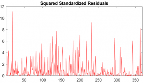
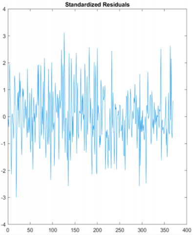
Figure 7 shows the distribution of the standardized residuals and the test for autocorrelation. It's clear that the series is stationary and does not suffer from signification autocorrelation.
(a)
(b)
(c)
(d)
Figure 7. Standard residuals series, distribution curves, ACF and PACF for squared standard residuals series
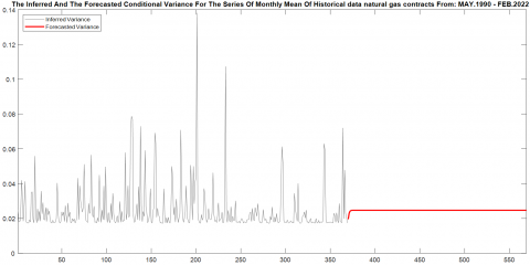
Figure 8 shows the conditional variance of the model and how it approaches the unconditional variance as the model shows stability over time. Figure 9 shows how closely the conditional variance approaches the unconditional variance indicating that the model has reached good stability.
Figure 8. Model-output conditional variance series and conditional variance forecasting
Figure 9. Conditional variance, its stability, and its approach to unconditional variance
(6) After verifying the readiness of the NAGARCH(1,1) model in the previous five stages, we will perform in this last stage the forecasting and plot the resulting conditional variance series from the NAGARCH(1,1) model and the forecasting conditions in Figure 8 and Figure 9. The conditional variance and its stability and its approach to the unconditional variance.
3.3 Analysis using the ARIMA-NAGARCH hybrid model
1. The data is entered and the original series is converted into a return series. As mentioned previously, the ARMA-NAGARCH mixture is modeled, and verify the stability of the mixture by dividing and testing the NAGARCH models and the stability of the ARMA models separately.
From Table 4, the best hybrid model is ARIMA(1,0,1)-NAGARCH(1,1), which achieves the lowest AIC and BIC values with data stability.
2. After we have chosen the best order for the model and verified its stability, we find the standard remainder series of using the infer command in MATLAB and we draw the quantum function, which is a visual examination of whether the series has a normal distribution or not.
Table 4. Stability test and values of AIC and BIC
|
ARMA(R,M,D)-NAGARCH(1,1) |
Stationary |
AIC |
BIC |
|
ARMA(1,0,0)-NAGARCH(1,1) |
Yes |
-337.4763 |
-314.0116 |
|
ARMA(1,0,1)-NAGARCH(1,1) |
Yes |
-347.7171 |
-320.3415 |
|
ARMA(1,0,2)-NAGARCH(1,1) |
Yes |
-347.3195 |
-316.0332 |
|
ARMA(1,0,3)-NAGARCH(1,1) |
Yes |
-346.8289 |
-311.6317 |
|
ARMA(1,0,4)-NAGARCH(1,1) |
Yes |
-345.0320 |
-305.9240 |
|
ARMA(2,0,0)-NAGARCH(1,1) |
Yes |
-342.0048 |
-314.6293 |
|
ARMA(2,0,1)-NAGARCH(1,1) |
Yes |
-347.0075 |
-315.7212 |
|
ARMA(2,0,2)-NAGARCH(1,1) |
Yes |
-346.8788 |
-311.6816 |
|
ARMA(2,0,3)-NAGARCH(1,1) |
Yes |
-345.0282 |
-305.9202 |
|
ARMA(2,0,4)-NAGARCH(1,1) |
Yes |
-343.1528 |
-300.1341 |
|
ARMA(3,0,0)-NAGARCH(1,1) |
Yes |
-340.5263 |
-309.2399 |
|
ARMA(3,0,1)-NAGARCH(1,1) |
Yes |
-346.7851 |
-311.5879 |
|
ARMA(3,0,2)-NAGARCH(1,1) |
Yes |
-345.0370 |
-305.9290 |
|
ARMA(3,0,3)-NAGARCH(1,1) |
Yes |
-343.0370 |
-300.0182 |
|
ARMA(3,0,4)-NAGARCH(1,1) |
Yes |
-341.7333 |
-294.8038 |
|
ARMA(4,0,0)-NAGARCH(1,1) |
Yes |
-339.4921 |
-304.2949 |
|
ARMA(4,0,1)-NAGARCH(1,1) |
Yes |
-343.3681 |
-300.3493 |
|
ARMA(4,0,2)-NAGARCH(1,1) |
Yes |
-341.8825 |
-294.9530 |
|
ARMA(4,0,3)-NAGARCH(1,1) |
Yes |
-322.1394 |
-304.2991 |
|
ARMA(4,0,4)-NAGARCH(1,1) |
No |
-319.9374 |
-304.3141 |
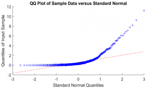
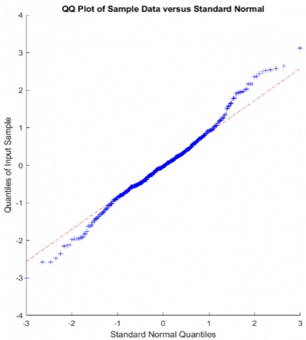
Figure 10 refers to plot standard remainder series and plot quantum function.
(a)
(b)
Figure 10. The standard residual series and the quantum function of the normal distribution
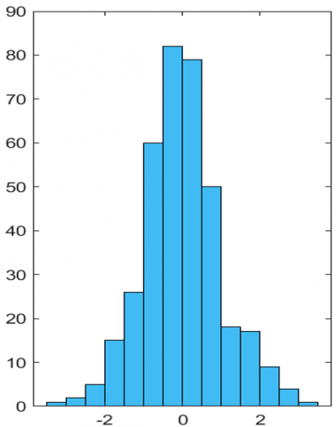
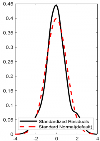
It becomes clear that the series forms a straight line next to the normal distribution line, and this confirms that the series is normally distributed. Figure 11 shows the distribution plot of the standard residual series compared to the plot of the normal distribution curve and the shape of the frequency distribution of the residual series as follows:
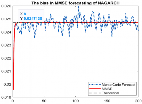
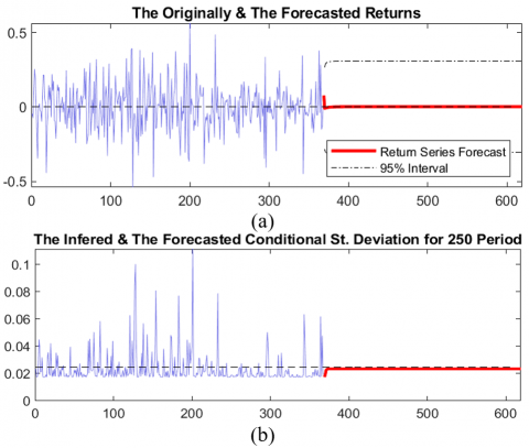
3. Make a prediction for the chosen model with 250 future steps, and the value of the unconditional mean is proved and fallen within the confines of the confidence interval which is specified by y±1.96/√MSE, where the MSE is the values of the mean squares of the predicted errors, which are observed to get closer to zero as the prediction steps increase. Figure 11 shows the mean least square errors for predictions on the return series as well as the conditional standard deviation predictions.
(a)
(b)
Figure 11. The normal distribution curve for the standard remainder series and the frequency distribution curve for the series
Figure 12. The series of original and predicted returns and the series of calculated and predicted variances
From Figure 12, the model shows acceptable performance in short-term forecasting, but may need improvement to accommodate dynamic changes in the long-term. Also, the conditional variance matches the actual behavior, which enhances the stability of the model.
4. The final stage of our modeling examined the predictive performance of the model used as we left out a calendar period of 12 months by using MSE. The model was used to predict return values for 11 future months and then return the return forecast values to their original values using the directive $d_t={ret} 2 {price}\left(r_t, 2.771\right)$, where 2.771 represents the last value of the training set.
Table 5 compares the actual and forecast values for natural gas returns over the 12 months. The forecasts are relatively close to actual values, but there are some differences that indicate poor model performance in predicating accurately.
Table 5. Monthly rate forecasts
|
No. |
Months |
Real Value |
Forecasting Value |
|
1 |
March |
2.608 |
2.7470 |
|
2 |
April |
2.931 |
2.7284 |
|
3 |
May |
3.055 |
2.7141 |
|
4 |
June |
3.650 |
2.7034 |
|
5 |
July |
3.914 |
2.6956 |
|
6 |
August |
4.377 |
2.6901 |
|
7 |
September |
5.867 |
2.6866 |
|
8 |
October |
5.426 |
2.6847 |
|
9 |
November |
4.567 |
2.6841 |
|
10 |
December |
3.730 |
2.6846 |
|
11 |
January |
4.874 |
2.6860 |
|
12 |
February |
4.406 |
2.6882 |
|
MSE |
2.7238 |
||
Figure 13 shows that the squared errors gradually approach zero in the long run, indicating that the model is trying to stabilize but may face challenges with high volatility. Low errors in the short run enhance the efficiency of hybrid ARIMA-NAGARCH model for near-term forecasts. However, there is a need to improve model strategies to address errors that appear in long- term forecasts.
Figure 13. Prediction errors of the model ARMA(1,0,1)-NAGARCH(1,1)
The results showed that the NAGARCH(1,1) model is the most stable and efficient among the other models based on the selection criteria (AIC and BIC). The model captures well the dynamics of natural gas price fluctuations and handles the asymmetric variance that characterizes these data. The results showed that the hybrid ARIMA(1,0,1)-NAGARCH(1,1) model performed better than the individual models when combining time trend analysis and conditional variance. The model performed well in short-term forecasting, with the forecast values being close to the true values. In the long run, the forecast errors (MSE) increased, indicating challenges in dealing with long-term dynamic fluctuations. The results of the model also showed that the conditional variance gradually approaches the unconditional variance, confirming the stability of the model and its ability to accommodate market fluctuations. The use of the local linear approximation (LLA) technique proved effective in analyzing the stability of the fixed points of the model. The research provides effective tools for analyzing natural gas price fluctuations, enabling decision makers in the energy and finance sectors to predict fluctuations and make informed decisions. The model can be extended to study other commodities and markets with similar dynamics.
We appreciative of the pioneering work of Dr. Azher Abas Mohammed, whose study on a similar subject was an inspiration that paved the way for this project.
[1] Engle, R.F. (1982). Autoregressive conditional heteroscedasticity with estimates of the variance of United Kingdom inflation. Econometrica: Journal of the Econometric Society, 50(4): 987-1007. https://doi.org/10.2307/1912773
[2] Glosten, L.R., Jagannathan, R., Runkle, D.E. (1993). On the relation between the expected value and the volatility of the nominal excess return on stocks. The Journal of Finance, 48(5): 1779-1801. https://doi.org/10.1111/j.1540-6261.1993.tb05128.x
[3] Higgins, M.L., Bera, A.K. (1992). A class of nonlinear ARCH models. International Economic Review, 33(1): 137-158. https://doi.org/10.2307/2526988
[4] Ozaki, T. (1985). 2 Non-Linear time series models and dynamical systems. In Handbook of Statistics, pp. 25-83. https://doi.org/10.1016/S0169-7161(85)05004-0
[5] Ali, N.E., Mohammad, A.A. (2023). Stability conditions of limit cycle for Gompertz Autoregressive model. Tikrit Journal of Pure Science, 28(2): 129-134. https://doi.org/10.25130/tjps.v28i2.1348
[6] Mohammad, A.A., Mudhir, A.A. (2020). Dynamical approach in studying stability condition of exponential (GARCH) models. Journal of King Saud University-Science, 32(1): 272-278. https://doi.org/10.1016/j.jksus.2018.04.028
[7] Noori, N.A., Mohammad, A.A. (2021). Dynamical approach in studying GJR-GARCH (Q, P) models with application. Tikrit Journal of Pure Science, 26(2): 145-156. http://doi.org/10.25130/tjps.26.2021.040
[8] Youns, A.S., Ahmad, S.M. (2023). Stability conditions for a nonlinear time series model. International Journal of Mathematics and Mathematical Sciences, 2023(1): 5575771. https://doi.org/10.1155/2023/5575771
[9] Hussien, A.M., Azher, M.A. (2022). New SIR model and vaccine rate with application. NeuroQuantology, 3050. https://doi.org/10.14704/nq.2022.20.7.NQ33383
[10] Abdulah, H.H., Azher, A.M. (2022). Stability study of exponential double autoregressive model with application. Neuroquantology, 20(6): 4812-4820.
[11] Bollerslev, T. (2008). Glossary to ARCH (GARCH). CREATES Research Paper 2008-49. http://doi.org/10.2139/ssrn.1263250
[12] Salim, A.J., Ebrahem, K.I. (2020). Studying the stability by using local linearization method. International Journal of Engineering Technology and Natural Sciences, 2(1): 27-31. https://doi.org/10.46923/ijets.v2i1.57
[13] Makridakis, S., Hibon, M. (1997). ARMA models and the Box-Jenkins methodology. Journal of Forecasting, 16(3): 147-163. https://doi.org/10.1002/(SICI)1099-131X(199705)16:3%3C147::AID-FOR652%3E3.0.CO;2-X
[14] Khalaf, N.S., Abdullah, H.H., Noori, N.A. (2024). The impact of overall intervention model on price of wheat. Iraqi Journal of Science, 853-862. https://doi.org/10.24996/ijs.2024.65.2.22
[15] Bollerslev, T., Engle, R.F., Nelson, D.B. (1994). ARCH models. Handbook of Econometrics, 4: 2959-3038. https://doi.org/10.1016/S1573-4412(05)80018-2
[16] Mohammad, A.A., Ghaffar, M.K. (2016). A study on stability of conditional variances for GARCH models with application. Tikrit Journal of Pure Science, 21(4): 160-169. https://doi.org/10.25130/tjps.v21i4.1069
[17] Bollerslev, T. (1986). Generalized autoregressive conditional heteroskedasticity. Journal of Econometrics, 31(3): 307-327. https://doi.org/10.1016/0304-4076(86)90063-1
[18] Barigozzi, M., Hallin, M. (2017). Generalized dynamic factor models and volatilities: Estimation and forecasting. Journal of Econometrics, 201(2): 307-321. https://doi.org/10.1016/j.jeconom.2017.08.010
[19] Abdullah, H., Noori, N.A. (2024). Comparison of non-linear time series models (Beta-t-EGARCH and NARMAX models) with radial basis function neural network using real data. Iraqi Journal for Computer Science and Mathematics, 5(3): 26-44. https://doi.org/10.52866/ijcsm.2024.05.03.003
[20] Al-Habib, K.H., Khaleel, M.A., Al-Mofleh, H. (2024). Statistical properties and application for [0, 1] truncated Nadarajah-Haghighi exponential distribution. Ibn AL-Haitham Journal for Pure and Applied Sciences, 37(2): 363-377. https://doi.org/10.30526/37.2.3349
[21] Al-Habib, K.H., Khaleel, M.A., Al-Mofleh, H. (2023). A new family of truncated Nadarajah-Haghighi-G properties with real data applications. Tikrit Journal of Administrative and Economic Sciences, 19(2): 311-333. http://www.doi.org/10.25130/tjaes.19.61.2.17
[22] Alanaz, M.M., Mustafa, M.Y., Algamal, Z.Y. (2023). Neutrosophic Lindley distribution with application for alloying metal melting point. International Journal of Neutrosophic Science (IJNS), 21(4): 65-71. https://doi.org/10.54216/IJNS.210407
[23] Naz, S., Al-Essa, L.A., Bakouch, H.S., Chesneau, C. (2023). A transmuted modified power-Generated family of distributions with practice on submodels in insurance and reliability. Symmetry, 15(7): 1458. https://doi.org/10.3390/sym15071458
[24] Salim, A., Ahmed, A. (2013). Stability analysis of a nonlinear autoregressive model of first order. Al-Rafidain Journal of Computer Sciences and Mathematics, 10(4): 135-145. https://doi.org/10.33899/csmj.2013.163561
[25] AlSaleem, N.Y.A. (2023). Network traffic prediction based on time series modeling. Iraqi Journal of Science, 4160-4168. https://doi.org/10.24996/ijs.2023.64.8.36