Gueye Pape El Hadji Abdoulaye*![]() | Deme Cherif Bachir
| Deme Cherif Bachir![]() | Basse Adrien
| Basse Adrien![]()
© 2025 The authors. This article is published by IIETA and is licensed under the CC BY 4.0 license (http://creativecommons.org/licenses/by/4.0/).
OPEN ACCESS
Flooding caused by the Senegal River during the 2024 rainy season has severely impacted several regions, particularly Saint-Louis, Matam, and their surrounding areas, disrupting infrastructure and livelihoods. In light of this growing vulnerability, anticipating climatic hazards has become essential. This article presents an innovative approach combining precipitation data from the UCSB-CHG/CHIRPS/DAILY collection and Sentinel-2 imagery to analyze and predict the Standardized Precipitation Index (SPI), with a focus on excessive moisture and flood risks. Although the SPI has historically been used for drought monitoring, it also proves relevant for detecting short-term precipitation excesses (SPI-1, SPI-3), which are potential indicators of flash floods. To enhance early detection of these extreme events, we developed a machine learning model based on Random Forest, optimized using the RandomizedSearchCV method. The results are promising: the model demonstrates excellent predictive power, with a Mean Squared Error (MSE) of 0.00072, a Root Mean Squared Error (RMSE) of 0.0268, a Mean Absolute Error (MAE) of 0.0184, and a coefficient of determination R² = 0.9991. These performances confirm the model's ability to anticipate risk zones, particularly in the agricultural lands along the Senegal River. This approach could be generalized to other watersheds vulnerable to extreme climatic events.
flood, Random Forest, RandomizedSearchCV, climate risk forecasting, SPI
Flooding caused by the Senegal River has had a significant impact on several regions of Senegal, particularly in the Saint Louis region and its surroundings, during the 2024 rainy sea son. These floods have severely disrupted the lives of residents, particularly in cities such as Matam and Saint-Louis, where many homes, roads, and agricultural lands were submerged. For example, in Bélli Diallo, victims often seek shelter outdoors, awaiting aid from local authorities, such as tents and temporary housing. These recurrent events highlight the vulnerability of these regions and the need to strengthen infrastructure and preventive measures against seasonal floods.
In this context, the combined use of satellite data (CHIRPS, Sentinel-2) and machine learning algorithms paves the way for proactive monitoring. Platforms such as NASA's Giovanni and EarthData provide access to time series of precipitation data that are well-suited for calculating the Standardized Precipitation Index (SPI). The paper by McKee et al. [1] introduced the Standardized Precipitation Index (SPI), a key tool for assessing drought and excessive moisture. SPI values help detect moisture anomalies: positive values indicate high moisture, while negative values signal drought.
Although SPI has traditionally been used to identify drought conditions, recent studies demonstrate its effectiveness in detecting excessive moisture, particularly over short temporal scales (SPI-1, SPI-3). Values exceeding +2.0 often indicate conditions conducive to flooding, especially when soils are already saturated.
In this study, we propose a flood risk forecasting model based on the Random Forest algorithm, applied to the Senegal River region. This model has been rigorously optimized using the RandomizedSearchCV method, resulting in a significant enhancement of its predictive performance. The results, notably a coefficient of determination R² = 0.9991, reveal an excellent agreement between predicted and observed values, confirming the relevance of this approach.
The remainder of this article is structured as follows: Section 2 reviews existing research on the use of AI and machine learning in climate risk forecasting; Section 3 presents the machine learning models employed and describes the study area; Section 4 details the methodology; Section 5 presents the results; Section 6 offers a thorough discussion; and finally, the conclusion and future perspectives are addressed in the Sections 7 and 8.
The study of climate risk forecasting increasingly relies on advanced artificial intelligence (AI) and machine learning (ML) models to improve the anticipation of extreme climate events. Numerous research efforts have explored diverse approaches, including machine learning algorithms, deep neural networks, hybrid models, and remote sensing techniques to enhance the prediction of climate risks such as droughts and floods, using indicators like the SPI.
This section highlights the strengths and limitations of each reviewed method:
To begin with, Türkeş et al. [2] presented a combined approach using statistical analysis and machine learning for drought forecasting in Central Anatolia, Turkey. The study shows that supervised learning models (e.g., neural networks, Random Forests) outperform traditional statistical models in accuracy. However, the reliance on localized historical climate data limits applicability to other regions.
In a similar effort, Abdullahi et al. [3] explored models like Extreme Learning Machine (ELM), Random Forest (RF), and Support Vector Regression (SVR) for drought prediction in Somalia. SVR outperforms others in accuracy and reliability but poses challenges due to data length requirements and model complexity.
Building on hybrid strategies, Oyounalsoud et al. [4] proposed a hybrid AI-based approach combining decision trees, SVMs, and neural networks using climate and soil moisture data. AI models generally outperform traditional indices, with decision trees showing strong drought correlation. The study's scope is limited to Australian data, restricting generalization.
Turning to flood forecasting, Zhang [5] introduced a flood risk prediction model based on logistic regression, k-means clustering, and Random Forests. It enhances accuracy by optimizing key indicators and risk classification but requires large datasets, limiting use in data-scarce regions. Interpretability remains an issue.
Earlier work by Deo and Şahin [6] applies Artificial Neural Networks (ANN) to forecast monthly SPI in Eastern Australia, outperforming traditional models by capturing nonlinear patterns. Yet, ANN models demand large datasets and are prone to overfitting if not properly tuned.
Expanding on neural approaches, Belayneh and Adamowski [7] developed hybrid models combining ANN with wavelet transforms for long-term drought prediction in the Awash River basin, Ethiopia. These hybrids surpass traditional models like ARIMA. However, parameter selection is complex, and models are data-intensive and computationally expensive.
Complementary to these studies, Choubin et al. [8] assessed AI techniques (ANFIS, M5P, MLP) using large-scale climate indices in an arid region of Iran. MLP performs best, especially with previous-month data. However, the study is geographically limited and lacks detailed analysis of specific indices.
Anshuka et al. [9] conducted a meta-analysis of statistical drought forecasting models based on the SPI, identifying that wavelet-based neural networks (WANN) provide the best performance with optimal accuracy at 12-month and 24-month timescales. The study highlights the importance of data preprocessing to improve prediction stability. However, results vary depending on geographic location and seasonal influences, limiting the universal generalizability of the mode.
A more integrative approach is seen in Masinde and Bagula [10], who presented a drought prediction and monitoring system for African smallholder farmers integrating seasonal forecasts and indigenous knowledge via ICT (e.g., sensors, mobile apps). Despite its high satisfaction rate in Kenya, it’s complex to maintain and deploy broadly.
Meanwhile, Danandeh Mehr et al. [11] proposed a CNN-LSTM hybrid for short-term drought forecasting, applied in Ankara. It outperforms benchmarks but was tested on only two stations, limiting generalization. Handling extreme events and spatial variability remains a challenge.
Addressing flood prediction challenges, Gyang et al. [12] explored integrating ML, GIS, and remote sensing for flood and rainfall forecasting in the U.S. The synergy enhances risk management but faces challenges in data heterogeneity, computational demands, and regulatory integration.
Along similar lines, Akinsoji et al. [13] presented a model combining ML and deep neural networks to predict water levels in agriculture. While precise, it demands extensive data and suffers from interpretability issues for non-experts.
From a river discharge perspective, Yaseen et al. [14] introduced an enhanced ELM model using Complete Orthogonal Decomposition (COD) for river discharge forecasting. It’s more accurate and robust than standard ELM/SVR models but requires large datasets and is hard to interpret.
Wavelet-based AI techniques are also explored by Soh et al. [15], who investigated WAANN and WANFIS models for SPEI prediction, showing improved accuracy via wavelet decomposition and AI. However, short-term predictions remain error-prone, and models are complex.
For satellite-based monitoring, Siddique and Ahmed [16] proposed CCD-3-CONV1D, a deep learning model for flood monitoring using Sentinel-1 SAR imagery. It improves change detection and flood prediction accuracy, but depends on high-quality data and complex image processing.
Shifting to a multidisciplinary approach, Onsay et al. [17] combined ML/econometrics and hermeneutic analysis to predict flood risks and assess disaster preparedness in the Bicol region. Socioeconomic vulnerability is emphasized, but the need for high-quality data and methodological integration of indigenous knowledge poses challenges.
Additionally, Naibi et al. [18] developed a hybrid LSSVM-SVCLR model to analyze drought-flood transitions in arid regions. Combining least squares SVM with spatially varying logistic regression, it improves robustness and captures spatial non-stationarity. However, its complexity and data demands hinder large-scale deployment.
On the time series side, Ding et al. [19] proposed a hybrid CEEMD-LSTM model that stabilizes time series and improves SPI forecasting across time scales, peaking at 24 months. Computational complexity and data quality remain hurdles.
A more architecture-focused solution is presented by Li et al. [20], who introduced the AGRS-LSTM-TRANSFORMER model combining attention-based graph structures, LSTM, and Transformer networks for flood prediction in the JINGLE watershed. It achieves high NSE scores (>0.905) but suffers from complexity, sensitivity to input data, and interpretability issues.
Furthermore, Farahmand et al. [21] created a spatio-temporal graph deep learning model for real-time urban flood prediction. Integrating physical and social data improves accuracy, but its complexity and data heterogeneity limit scalability.
In a complementary study, Roudbari et al. [22] developed a graph neural network (LocalFloodNet) and a digital twin prototype for urban flood forecasting in Terrebonne, Québec. It supports scenario simulation and decision-making, but requires precise data and is computationally demanding.
Likewise, Situ et al. [23] integrated LSTM-SEGNET-MSA and ES-Deeplab in a deep learning model for urban flood risk assessment. It effectively merges spatial and temporal features, improving prediction and economic loss estimation, yet still faces computational and data challenges.
To push prediction accuracy further, Wang et al. [24] combined STGCN and Graph WaveNet with attention mechanisms for flood prediction, reducing peak error by 0.26%. Though highly precise, it demands detailed hydrological data and is computationally intensive.
Lastly, Bouaziz et al. [25] highlighted the efficiency of ELM in SPI prediction using remote sensing in arid regions. While performance is promising (R² between 0.7-0.8), it struggles with low-quality or noisy remote sensing data and lacks robustness in handling complex variable interactions. Given these observations and the inherent complexity of predicting climate risks from multiple environmental variables, we developed a machine learning-based solution that integrates several powerful algorithms (Random Forest, XGBoost, SVR, ELM) to enhance the accuracy and robustness of forecasts.
This approach is further strengthened by data augmentation techniques and feature importance analysis, providing a reliable and interpretable predictive framework to support the sustainable management of water resources in the Senegal River Basin.
In this work we use supervised learning models: XGBoost, Random Forest and SVR and an ELM model. Random Forest and XGBoost are ensemble tree models used for complex regression and classification tasks, while SVR is distinguished by its geometric approach and is often more widely used when the data is smaller or better structured. ELM is a single-hidden-layer neural network that is fast to train thanks to random initialization of internal weights and analytical learning of output weights. It is suitable for regression and classification tasks, particularly where speed of learning and low computational complexity are priorities.
3.1 XGBoost
XGBoost [26] is a boosting algorithm that optimises the performance of decision tree models. It is a supervised learning method that builds models by adding several weaker models (decision trees). XGBoost uses regularisation to avoid overlearning and offers very accurate predictions. This model is extremely popular due to its speed of execution and exceptional performance on tabular datasets. XGBoost is particularly effective for classification and regression problems, especially where there are complex interactions between features.
The objective of XGBoost is to minimise the following loss function:
$L(\theta)=\sum_{i=1}^n \ell\left(\mathrm{y}_{\mathrm{i}}, \hat{y}_{\mathrm{i}}\right)+\sum_{i=1}^n \Omega\left(f_k\right)$ (1)
where,
$\ell\left(\mathrm{y}_{\mathrm{i}}, \hat{y}_{\mathrm{i}}\right)$ is the loss function (e.g., squared error or logistic loss) between the true value yi and the predicted value $\hat{y}_i$.
Ω(fk) is the regularization term applied to the complexity of the model.
fk is a decision tree.
K is the number of trees in the model.
θ are the model parameters.
The training process of XGBoost focuses on minimizing this objective function using gradient descent techniques.
3.2 Random Forest
Random Forest [27] is a supervised learning algorithm based on the decision tree method. It is a set model that constructs multiple decision trees during training and combines them to produce a more robust prediction that is less likely to overlearn the training data. Each tree in the forest is built using a random subset of the features and training data. This diversity of trees improves performance and reduces the risk of overlearning, making the Random Forest a particularly powerful model for regression and classification problems. The objective of a decision tree in the forest is to minimise the loss function L, such that:
$f(x)=\frac{1}{T} \sum_{t=1}^T f_t(x)$ (2)
where,
ft(x) is the prediction made by the t-th decision tree,
T is the total number of trees in the forest.
For a single decision tree ft(x), the training process minimises the following loss function:
$L=\sum_{i=1}^n\left(y_i-f_t\left(x_i\right)\right)^2+\lambda \sum_j\left\|\theta_j\right\|_2^2$ (3)
where:
yi are the true values,
xi are the feature vectors,
θj are the model parameters.
3.3 SVR
SVR [28] is a regression model based on support vector machines.
The goal of SVR is to find a function f(x) that predicts the values of the data while maintaining a certain tolerance for error.
The objective is to maximize the margin around the prediction function while limiting the errors. SVR is particularly useful, when the relationship between the input variables and the output is nonlinear, and is therefore often used for complex time series where the relationships between the variables are subtle and not obvious.
The goal of SVR is to minimize the following function, which incorporates both error tolerance and model complexity
$\min _\theta\left(\frac{1}{2}\|w\|^2+C \sum_{i=1}^n \xi i\right)$ (4)
Under constraints:
$y_i-f\left(x_i\right) \leq \varepsilon+\xi i$ (5)
$f\left(x_i\right)-y_i \leq \varepsilon+\xi i$ (6)
$\xi i \geq 0, i=1,2, \ldots, n$ (7)
where:
yi is the true value of the i-th drive point,
f(xi) is the prediction for the i-th training point,
w is the weight vector, and
C is a regularisation parameter,
$\xi_i$ are the release variables, which allow a certain degree of flexibility in the model to manage errors. The function f(x) is generally defined as a linear combination of the kernel functions in the case of a non-linear SVR. In the case of language models, this loss is often the loss of cross-entropy between the predicted sequence and the true sequence.
3.4 ELM
ELMs [29] are single hidden layer neural networks (SLFNs) in which the weights between the input and the hidden layer are randomly initialised and not adjusted during learning. Only the weights between the hidden layer and the output are learned, which allows extremely fast training by solving a linear problem.
Given a training set $\left\{\left(x_i, t_i\right)\right\}_{i=1}^N$ with $x_i \in \mathbb{R}^n$ the inputs and $t_i \in \mathbb{R}^m$ target outputs.
An ELM with L hidden neurons performs the following modelling:
$f(x)=\sum_{j=1}^L \beta \operatorname{jg}\left(w_j^T \mathrm{x}+\mathrm{b}_j\right)$ (8)
where:
g(·) is the activation function (ex.sigmoïde, ReLU, sinus).
$w_j \in \mathbb{R}^n$ is the input weight vector of the j-th hidden neuron.
$b_i \in \mathbb{R}$ is the bias of the j-th hidden neuron.
$\beta_j \in \mathbb{R}^m$ is the vector of output weights associated with the jth neuron. In matrix notation, we give
$H=\left(\begin{array}{ccc}g\left(w_1^T x_1+\mathrm{b}_1\right) & \cdots & g\left(w_L^T x_1+\mathrm{b}_L\right) \\ \vdots & \ddots & \vdots \\ g\left(w_1^T x_N+\mathrm{b}_1\right) & \cdots & g\left(w_j^T x_N+b_L\right)\end{array}\right) \in \mathbb{R}^{N \times L}$ (9)
And we're looking to solve
$H \beta=T$ (10)
where:
$\beta \in \mathbb{R}^{L \times m}$ is the output weight matrix to be estimated.
$T \in \mathbb{R}^{N \times m}$ is the target matrix.
The optimal solution (in the least squares sense) is obtained by pseudo-inverse:
$\beta=H^{\dagger} \mathrm{T}$ (11)
where, $H^{\dagger}$ is the Moore-Penrose pseudo-inverse of the H matrix. This formalism enables extremely fast learning without iterations, while maintaining good performance for many classification and regression tasks.
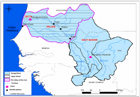
The Senegal River, 1800 km long, is the second largest river in West Africa. Its basin, covering 300,000 km², stretches from the Fouta Djallon mountains to the north of Senegal as shown in Figure 1. Born of the confluence of the Bafing and Bakoye rivers in Mali, the river is of ecological and economic importance to the countries it flows through. Its main component, the Bafing, rises near Mamou in Guinea and flows through fertile plains before reaching the Atlantic Ocean.
Figure 1. Senegal River (www.google.com)
4.1 Analysis of precipitation variability in Senegal using the SPI index
In this study, we use data from the UCSB-CHG/CHIRPS/DAILY (Climate Hazards Group InfraRed Precipitation with Station Data) collection, which provides daily rainfall estimates on a global scale. These data are obtained by combining satellite observations and measurements from weather stations, thereby improving coverage and accuracy, particularly in areas where there are few stations. In addition, this collection offers a long time series, going back to 1981, which is essential for analysing climate trends and extreme events. We have calculated the SPI from this collection to assess the variability of rainfall around the Senegal River over the period from June 1990 to October 2024.
4.1.1 Data collection
The objective of CHIRPS is to provide precipitation data at a spatial resolution of 0.05° (≈ 5 km) and on a daily scale. This data is used to analyse precipitation trends and to study climatic phenomena such as droughts and floods. The study area covers approximately 300,000 km2, divided into 25 km2 zones, each zone corresponding to a raster pixel. For each pixel, we extract:
-Latitude and longitude,
-The calculated SPI value.
4.1.2 Data preparation
The precipitation data, extracted from the CHIRPS collection, cover the period from 1990 to 2024. For the analysis, we focus on the rainy season, from June to October. The calculation of the Standardized Precipitation Index (SPI) is used to assess the climatic conditions associated with drought and excess precipitation.
4.1.3 Calculation of the SPI (standard method)
The calculation of the SPI follows the standard method proposed by McKee et al. [1], which involves the following steps:
-Calculation of mean and standard deviation: For each month, historical rainfall data are used to calculate:
-The average precipitation, noted as: µ
-The standard deviation of precipitation, denoted σ
•Standardisation:
The SPI is obtained from the following formula:
SPI $=\frac{(X-\mu)}{\sigma}$ (12)
where:
X is the observed precipitation for a given month.
$\mu$ is the historical average rainfall for the month.
$\sigma$ is the corresponding standard deviation.
• Interpretation:
SPI =0: normal conditions,
SPI >0: excess rainfall,
SPI < 0: drought conditions, the severity of which increases with more negative values.
4.1.4 Our method of calculating the SPI
Unlike the conventional monthly method, we calculated the SPI on a daily basis, for each com day taken between June and October (the rainy season in Senegal), by comparing the daily rainfall value with the average rainfall for the same period over the previous years.
4.1.5 Visualisation and analysis of SPI calculation results
The results of the SPI calculation are analysed and displayed in several ways:
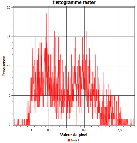
-Histogram of SPI values: shows the distribution of SPI indices over the entire study area.
Figure 2 shows that the most frequent SPI values are between -0.7 and +0.7, indicating near-normal conditions. The maximum value observed is +1.88, and the minimum is -1.46. According to Table 1, extreme conditions (drought or humidity) occurred in less than 5% of cases.
Figure 2. Histogram of SPI values extracted from .tif images
Table 1. Classification of climatic sequences according to the SPI index [1]
|
SPI Values |
Category |
|
2 and above |
Extremely wet |
|
1.5 to 1.99 |
Very wet |
|
1 to 1.49 |
Moderately wet |
|
-0.99 to 0.99 |
Near normal |
|
-1 to -1.49 |
Moderately dry |
|
-1.5 to -1.99 |
Very dry |
|
-2 and below |
Extremely dry |
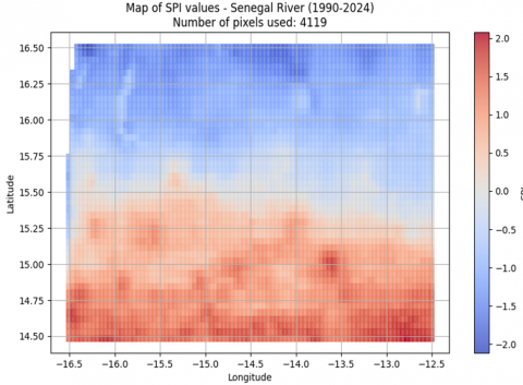
-SPI pixel map: represents the spatial variability of rainfall in the Senegal River basin.
Figure 3. Map of pixels in the Senegal river basin with associated SPI values
Figure 3 illustrates the spatial distribution of SPI values, making it possible to identify drier or wetter areas. These results are used as input variables in prediction models, in particular the Random Forest model, to assess climate risks.
4.2 Obtaining the dataset
The analysis is based on the use of Google Earth Engine (GEE) to extract and process satellite data covering the Senegal River valley from June 1990 to October 2024. After initializing GEE (ee.Initialize()), a study area is defined as a polygon encompassing the region of interest. Sentinel-2 images are loaded, retaining only the essential spectral bands: B2 (blue), B3 (green), B4 (red), and B8 (near-infrared - NIR). At the same time, precipitation data are extracted from the CHIRPS dataset, and the total sum of precipitation over the period is calculated. Vegetation indices (NDVI, NDWI, MSAVI) and spectral bands (B2, B3, B4, B8, etc.) are derived from Sentinel-2 imagery. The following sub-sections describe how temporal and spatial correspondence between these two datasets was managed.
4.2.1 Temporal correspondence
CHIRPS data offer a daily temporal resolution, allowing the retrieval of precipitation information for each day in the study period (1990-2024). Daily rainfall values were extracted and used to compute the SPI, specifically for the months of June to October, to better capture the season of high rainfall activity in the Senegal River region. Sentinel-2 data are acquired every 5 to 10 days, depending on weather conditions and cloud cover. These images were used to calculate vegetation indices (NDVI, NDWI, MSAVI) and extract specific spectral bands (B2, B3, B4, B8), which provide insights into vegetation cover, soil moisture, and other environmental variables, albeit at a coarser temporal frequency compared to CHIRPS.
Thus, while CHIRPS provides daily granularity, Sentinel-2 data are less frequent (5-10 days), requiring temporal aggregation of vegetation indices and spectral bands to align with the precipitation data.
4.2.2 Spatial correspondence
CHIRPS data are available at a spatial resolution of 5 km per pixel, which is relatively coarse compared to Sentinel-2 imagery. This resolution allows analysis of precipitation trends across larger geographical regions and is suitable for regional-scale applications.
Conversely, Sentinel-2 images offer a much finer spatial resolution, ranging from 10 to 60 meters depending on the spectral band. For example, the visible bands (B2, B3, B4) have a resolution of 10 meters, and the near-infrared bands a resolution of 20 meters. This high spatial precision allows for detailed analysis of land cover and vegetation indices like NDVI, NDWI, and MSAVI.
Therefore, CHIRPS provides a broader overview at 5 km resolution, whereas Sentinel-2 enables detailed landscape-level observation at pixel resolutions ranging from 10 to 20 meters.
4.2.3 Management of temporal and spatial correspondence
Due to the differences in temporal and spatial resolutions, a harmonization process was necessary:
-Daily CHIRPS precipitation data were averaged over time intervals corresponding to Sentinel-2 acquisition periods (approximately every 5 to 10 days).
-Vegetation index values from Sentinel-2 were extracted over the geographical areas covered by CHIRPS pixels (5 km), taking into account the finer spatial resolution of Sentinel-2.
The two datasets were then merged into a single Excel file, enabling a comparative analysis of SPI (from CHIRPS precipitation data) and vegetation indices (NDVI, NDWI, MSAVI) as well as spectral bands (B2, B3, B4, B8) from Sentinel-2.
This fusion allowed a direct comparison between SPI values and vegetation indices, while considering the differences in temporal and spatial resolutions between the two sources.
4.2.4 Vegetation indices calculation
Several vegetation indices were computed from Sentinel-2 imagery:
NDVI $=\frac{\text { NIR }- \text { Rouge }}{\text { NIR }+ \text { Rouge }}$ (13)
NDWI $=\frac{\text { Vert }- \text { NIR }}{\text { Vert }+ \text { NIR }}$ (14)
$E V I=2.5 \times \frac{N I R-{ Rouge }}{N I R+6 \times { Rouge }-7.5 \times { Bleu }+1}$ (15)
$\begin{gathered}M S A V I= \frac{2 \times N I R+1-\sqrt{(2 \times N I R+1)^2-8 \times(N I R- { Rouge })}}{2}\end{gathered}$ (16)
These indices were averaged over the entire period and then merged with precipitation data. A total of 200 random points were generated within the study area, and vegetation index values were extracted at a spatial resolution of 5 km.
4.2.5 SPI calculation
The combined dataset was converted into a Pandas DataFrame. The SPI was then calculated using the following formula:
$S P I=\frac{\text { TotalPrecip }-\mu}{\sigma}$ (17)
where, μ is the mean and σ is the standard deviation of precipitation over the entire study period.
4.2.6 Exporting the results
All results were exported into an Excel file. The data were extracted from .tif raster images and organized into a tabular format, with each row representing the values for a given pixel. The dataset includes 200 records corresponding to the sampling points and is intended for use in climate risk modeling, including drought monitoring and water resource management.
4.3 Training of prediction models
We tested several machine learning models to predict SPI values, including Random Forest, XGBoost and Support Vector Regression (SVR), and compared our models to an Extreme Learning Algorithm (refer to Table 2).
The process for predicting SPI values with machine learning models involves several key steps. First, the data is loaded from the source followed by preprocessing, where relevant features and the target variable (SPI) are selected. Next, the data is split into training 80% and testing sets 20%. Then, models Random Forest, XGBoost, and SVR, are optimized and trained using cross validation. After training, predictions are made on the test data. Finally, model performance is evaluated using metrics like MSE, RMSE, MAE, and R2, and the results are visualized through graphs.
Table 2. Models, authors, references, strengths and weaknesses
|
Model |
Reference |
Forces |
Weakness |
|
XGBoost |
[26] |
Excellent performance on tabular data, management of missing values |
Sensitive to overfitting if incorrectly set |
|
Random Forest |
[27] |
Robust, reduces overlearning, easy to interpret. |
Less efficient on very large data sets |
|
SVR |
[28] |
Good for small data sets with a clear structure |
Costly in terms of computing time and memory for large datasets |
|
ELM |
[29] |
Very fast in training, good for the time |
Less robust, highly dependent on random initialisation |
5.1 Data pre-processing
Data pre-processing is an essential step in ensuring the quality and relevance of the results obtained by the regression models.
In this study, the following steps were carried out:
Data loading:
The data were extracted from an Excel file containing various environmental variables and the SPI used as the target variable.
Variable selection:
Nine explanatory variables were selected for model training:
B2, B3, B4, B8, EVI, MSAVI, NDVI, NDWI and TotalPrecip.
The variable to be predicted is the SPI.
Splitting of the dataset:
The dataset was split into two subsets: 80% of the data for model training and 20% for model evaluation. This separation was carried out in a random but reproducible manner, by setting a random_state of 42.
Robustness to noise:
In order to test the resilience of the models, Gaussian noise was artificially introduced into the input data (the explanatory variables). More specifically, for each level of noise, random noise of mean zero and standard deviation proportional to the standard deviation of the variables was added to the test set, according to the formula:
$S P I=\chi_{\text {bruité }}=\chi_{\text {test }}+\aleph\left(0, \sigma^2\right) \frac{\text { TotalPrecip }-\mu}{\sigma}$ (18)
where, $\sigma=\alpha \cdot \operatorname{std}(\mathrm{X_{test}})$, with α varying between 0% and 55% in 5% steps. This perturbation is applied only to the input characteristics, and not to the target variable (SPI), in order to assess the robustness of the models to noisy sensors or potential measurement errors.
The aim of this pre-processing is to ensure that the data supplied to the models is consistent, relevant and representative of the phenomena under study, while enabling a rigorous assessment of their stability in real-life conditions.
5.2 Comparative evaluation and optimisation of SPI prediction models
The analysis looked at performance before and after hyperparameter optimisation, measuring the classic metrics: Mean Squared Error (MSE), Root Mean Squared Error (RMSE), Mean Absolute Error (MAE) and coefficient of determination (R2). A significant difference between training and test performance would have been an indicator of over-fitting. The test set was strictly isolated throughout the model development process, including hyperparameter fitting. Specifically, we adopted a cross-validation (3-folds) only on the training set to select the best hyperparameters. The test set was used only once, at the very end of the process, to obtain an unbiased estimate of the model's final performance.
5.2.1 Optimising models by hyperparameter selection
Each machine learning model Random Forest, XGBoost, SVR has been optimised using RandomizedSearchCV to efficiently explore the hyperparameter space. For Random Forest, the parameters tested include the number of trees (n_estimators), the maximum depth (max_depth) and the minimum division sizes. The XGBoost model was refined according to parameters such as the learning rate (learning_rate), the depth (max_depth) and the subsampling (subsample). Finally, for SVR, kernels (kernel), regularisation (C) and the gamma parameter were explored in order to optimise cross-validation performance (Table 3).
Table 3. Hyperparameters before optimization
|
Models |
Hyperparameters |
|
Random Forest |
n_estimators=[50, 100, 200], max_depth=[10, 20, 30, None], min_samples_split=[2, 5, 10], min_samples_leaf=[1, 2, 4] |
|
XGBoost |
n_estimators=[50, 100, 200], learning_rate=[0.01, 0.05, 0.1, 0.2], max_depth=[3, 6, 10], subsample=[0.7, 0.8, 1.0] |
|
SVR |
C=[0.1, 1, 10, 100], gamma=['scale', 'auto', 0.01, 0.1, 1], kernel=['rbf', 'linear'] |
Training with RandomizedSearchCV is a loop of random tests of hyperparameters, coupled with cross-validation. XGBoost is trained by building a sequence of decision trees, where each new tree corrects the errors of the previous ones, and its hyperparameters are optimised via cross-validation to maximise performance. SVR is trained by finding a function that predicts target values within a tolerable margin of error, possibly transforming the data with a kernel, and its parameters are adjusted using random search to improve generalisation. After optimisation, we obtain the following hyperparameters (Table 4).
Table 4. Hyperparameters after optimisation
|
Models |
Best Parameters |
|
Random Forest |
n_estimators=100, max_depth=10, min_samples_split=2, min_samples_leaf=2 |
|
XGBoost |
n_estimators=100, learning_rate=0.1, max_depth=6, subsample=0.8 |
|
SVR |
kernel=linear, gamma=1, C=1 |
We used one hundred fixed neurons and a sigmoid activation function for the ELM model.
5.2.2 Comparative evaluation of model performance
(1) Model performance
Model performance is compared between training and testing according to the following metrics: MSE, RMSE and R² (Table 5).
(2) Analysis and interpretation
The comparative analysis shows that the Random Forest and XGBoost models perform best on test data. Their ability to generalise is confirmed by the small difference between training and test performance. In particular, Random Forest shows great stability and robustness (R2 = 0.99899 in test), making it the best candidate for SPI predictions. XGBoost, despite an excellent performance in training (R2 = 0.99999), shows a slight deviation in testing, suggesting minimal overlearning. SVR performed less well overall and showed some variability in the error, probably due to sensitivity to the choice of kernel. As for the ELM model, it suffers from significant numerical problems (overflows in the sigmoid function), making its training unstable. This is reflected in an R2 of just 0.938 in test, which is significantly lower than the other models. Random Forest is therefore selected as the best compromise between accuracy, stability and generalisation capacity.
5.3 Importance of selected characteristics
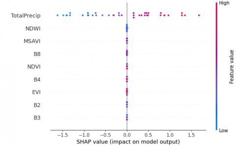
To better understand the influence of explanatory variables on the prediction of the SPI index, an interpretability analysis based on SHapley Additive exPlanations (SHAP) values was conducted. This method allows for both local and global attribution of each feature’s contribution to the model’s output.
Figure 4. SHAP values for the test set (Random Forest model)
Figure 4 shows the SHAP values associated with the variables in the model. Each point represents an instance of the test set. The horizontal position indicates the effect of the variable on the prediction (SHAP value), while the colour reflects the actual value of the variable (blue for a low value, red for a high value).
-TotalPrecip is by far the most influential characteristic. High values of total precipitation (in red) tend to strongly increase the SPI (positive SHAP impact), which is consistent with the hydrological nature of the SPI index.
-NDWI and MSAVI come second and third. NDWI (moisture index) has a moderate influence, generally negative for low values. This reflects the link between surface humidity and water stress detected by the SPI.
-Spectral bands (B4, B8, etc.) and vegetation indices such as NDVI or EVI have a weaker, but not negligible effect. Their contribution is mainly centred around zero, which suggests that they modulate the prediction without dominating it.
-The fact that several variables have points distributed on either side of the zero axis indicates that their effect on the prediction varies according to the observations (positive or negative impact depending on the situation).
This analysis confirms the relevance of the choice of environmental variables used in the models, in particular the crucial importance of the variable TotalPrecip, which acts as the main predictor of SPI in this river context.
5.4 Assessment of model robustness
5.4.1 Analysis of model robustness to noise
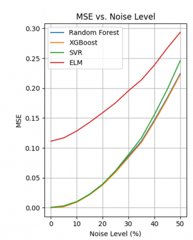
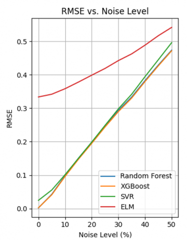
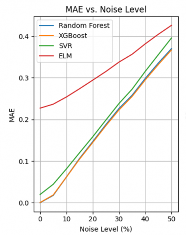
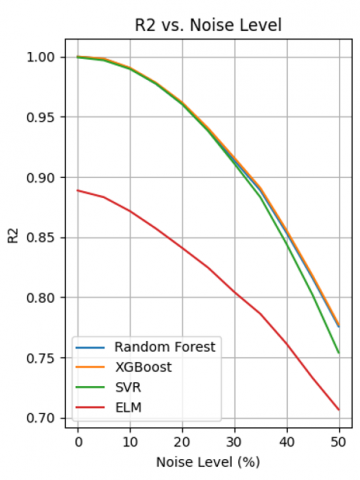
The MSE, RMSE, MAE and R² curves in Figure 5 allow us to assess the robustness of four models (Random Forest, XGBoost, SVM, ELM) to different levels of Gaussian noise.
Here are the main observations:
General trends:
All errors (MSE, RMSE, MAE) increase with noise, while the R² decreases, as theoretically expected. The speed of degradation varies significantly between models.
Model comparison:
-Random Forest & XGBoost: Ensemble models showing excellent robustness. The errors increase slowly and the R² remains high even at 50% noise (≈ 0.85-0.90). Their ability to aggregate several predictions enables them to limit the impact of noise.
Table 5. Training vs. test performance
|
Model |
MSE (Train) |
RMSE (Train) |
R² (Train) |
MSE (Test) |
RMSE (Test) |
R² (Test) |
|
Random Forest |
0.00067 |
0.02584 |
0.99936 |
0.00078 |
0.02786 |
0.99899 |
|
XGBoost |
0.000007 |
0.00271 |
0.99999 |
0.00124 |
0.03518 |
0.99840 |
|
SVR |
0.00289 |
0.05379 |
0.99724 |
0.00229 |
0.04781 |
0.99704 |
|
ELM |
- |
- |
- |
0.04778 |
0.21859 |
0.93816 |
Figure 5. Evolution of the MSE, RMSE and MAE of the models in the face of Gaussian noise
-SVM: Sensitive to noise, especially visible on MAE and R². The latter drops to ≈ 0.80 at 50% noise. This sensitivity could stem from the rigidity of decision margins.
-ELM: The most vulnerable, with a sharp increase in errors and a significant drop in R² (≈ 0.70 at 50% noise). Its simple architecture and lack of explicit regularisation make it more prone to overfitting.
-Consistency of metrics:
The error and R² curves are consistent: as the error increases, the R² decreases. XGBoost systematically maintains lower errors and higher R², illustrating a good compromise between performance and robustness.
-Curve stability:
Random Forest and XGBoost have regular, predictable curves. ELM shows more marked fluctuations (especially in MAE and R²), reflecting instability in the face of intermediate noise (20-40%).
5.4.2 Interpretation of noise robustness results
Adding Gaussian noise to the data makes it possible to simulate a realistic environment where the data is imperfect or disturbed. In this context, the performance of the models varies according to their ability to manage uncertainty. The error metrics (MSE, RMSE, MAE) measure the gap between predictions and the ground truth, while the R² assesses the proportion of variance explained by the model.
-Expected behaviour: The increase in errors (MSE, RMSE, MAE) and the decrease in R² with the increase in noise is theoretically expected. This indicates that the models find it more difficult to produce accurate predictions when the data becomes less reliable.
-Ensemble models (Random Forest, XGBoost): Their resistance to noise is explained by their architecture. These models are based on the combination of many weak learners (decision trees) to produce a global prediction. This aggregation cushions the effect of noise, because point errors are "diluted" in the ensemble. Their error curves progress slowly, and the R² remains high, showing that they retain a good capacity for generalisation.
-SVM: SVMs use rigid margins to separate the data. In the presence of noise, outliers can have a disproportionate effect on these margins. This leads to a rapid degradation in performance, particularly in MAE, suggesting that the model makes more significant errors on certain perturbed data.
-ELM: ELM is based on a very simple neural network architecture (a single hidden layer with random initial weights). It does not incorporate an explicit regularisation mechanism, which makes it vulnerable to noise. The fact that its curves are unstable and that the R² drops rapidly indicates a high variability in performance according to noise levels, typical of a model that is too sensitive to variations in the data.
-R² as an overall indicator of robustness: The progressive loss of R² reflects the decreasing ability of the models to capture the structure of the data. A robust model is one whose R² falls slowly, which is the case for Random Forest and XGBoost. This confirms that these models retain a high explanatory capacity even when the environment becomes noisy.
5.5 Prediction of SPI values with the best models Random Forest, SVR, XGBoost
In this section, we present the results obtained by predicting the values of the SPI using the three machine learning models: Random Forest, XGBoost and SVR. These models were evaluated on a test set and compared in terms of several evaluation criteria, including MSE, MAE, RMSE and coefficient of determination R2.
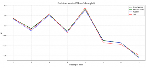
Figure 6. Predictions of SPI values
Figure 6 shows the evolution of the SPI indicator as a function of the samples in the test dataset. The x-axis represents the indices of the samples, while the y-axis shows the predicted values of the SPI. The curves of the models (Random Forest, XGBoost, SVR) are plotted with a transparency of 0.7, allowing their predictions to be compared with the actual SPI values (shown as dotted lines). The aim is to observe how each model follows the trend of the actual values and to assess the quality of the prediction for each sample.
Good performance can be seen when the curves of the models are close to the actual values, indicating a low prediction error. These visualisations help to understand the ability of each model to generalise and correctly predict SPI trends over the test set.
Random Forest proved to be the best model of the three, with an R2 of 0.9991, meaning that it explained 99.91% of the variance in the data. This model performed exceptionally well in terms of accuracy, with low prediction errors, making it a robust solution for SPI prediction. On the other hand, although XGBoost also performed remarkably well, with an R2 of 0.9984, it lagged slightly behind the Random Forest model. The SVR model, although effective, has a lower R2 of 0.9971, indicating that its ability to explain the variance in the data is slightly lower than that of the other two models.
These results show that, although all the models perform at a high level, Random Forest is the most suitable for predicting the SPI in this context, closely followed by XGBoost. The accuracy of the predictions and the low variability of the errors in the case of Random Forest make it the optimal choice for reliable and robust predictions. However, XGBoost remains an interesting alternative, notably because of its ability to model complex relationships while being slightly faster to train.
The results obtained clearly demonstrate the superiority of ensemble models, in particular Random Forest and XGBoost, in predicting the SPI from satellite and environmental data. These models not only have a very good predictive capacity under normal conditions, but are also remarkably robust in the face of disturbances simulating instrumental noise or measurement inaccuracies.
6.1 Predictive performance
Of all the models tested, Random Forest showed the best overall performance with an R2 close to 0.999 on the test set. This result reflects its exceptional ability to model the relationship between the explanatory variables (mainly TotalPrecip, NDWI and MSAVI) and the SPI. The XGBoost model, while performing slightly less well in test, retains a very high level of accuracy, but appears to be slightly more prone to overlearning, as indicated by the greater discrepancy between training and test scores.
6.2 Interpretability
The SHAP analysis made it possible to clarify the impact of the different variables on the predictions. The central role of TotalPrecip confirms the validity of the model, as this variable is directly linked to the nature of the SPI. Similarly, the water (NDWI) and vegetation (MSAVI, NDVI) indices play a relevant role, albeit a secondary one. This explanatory stage strengthens the credibility of the models used, particularly in terms of decision support for hydrological management.
6.3 Robustness to perturbations
Faced with increasing levels of Gaussian noise, the ensemble models showed a slow and gradual degradation in performance. This confirms their stability and their suitability for use in a real environment, where the data is rarely perfect. Conversely, the ELM proved to be unstable and unreliable, while the SVR, although more robust than the ELM, remains more sensitive to noise than RF or XGB.
6.4 Limitations of the ELM model
The ELM, although theoretically attractive for its speed of training, was unable to compete with the other algorithms in this context. Its numerical instability, linked in particular to the sigmoid function and the absence of effective regularisation, made it unsuitable for accurate prediction of the SPI on noisy data. This suggests that more advanced or hybrid versions of ELM could be considered for future experiments.
This study has shown that it is possible to predict the SPI index with a high degree of accuracy using machine learning models and environmental variables derived from satellite data. The Random Forest model emerged as the most robust and accurate solution, capable of generalising efficiently while maintaining remarkable stability even in the presence of significant noise. The results also highlight the crucial importance of certain variables, in particular TotalPrecip, whose major influence was confirmed by the SHAP analysis. The ability of the models to maintain high performance despite deliberate degradation of data quality attests to their potential in practical scenarios, where measurement errors are common. However, some models such as ELM have shown their limitations, suggesting the need to continue exploring more sophisticated architectures or adapted regularisation mechanisms to improve their reliability. Looking ahead, the integration of additional spatio-temporal data (such as soil or atmospheric humidity data), as well as the generalisation of models to other river basins, could pave the way for more comprehensive, dynamic and operational hydrological forecasting systems.
Although the results obtained in this study are promising, several avenues for improvement and future research deserve to be explored in order to further optimise SPI prediction and gain a better understanding of the underlying climate dynamics.
-Integration of additional data: One of the most interesting avenues would be to enrich the models with additional data, such as global climate indices (e.g. normalised precipitation index, temperature data, soil moisture), as well as socio-economic data. The integration of multivariate data could improve the accuracy of predictions and make it possible to extend model applications to wider scales.
-Improving the generalisability of the models: An important prospect would be to work on improving the generalisability of Random Forest and XGBoost. Although these models performed exceptionally well on training and test data, a slight over-fitting was observed. More advanced regularisation techniques, such as reducing tree depth, more rigorous feature selection or the application of more robust ensemble methods, could be explored to avoid this over-fitting.
We would like to express our sincere gratitude to the IMTICE Research Group at Alioune Diop University in Bambey, as well as to ANACIM and the Ministry of Agriculture of Senegal.
[1] McKee, T.B., Doesken, N.J., Kleist, J. (1993). The relationship of drought frequency and duration to time scales. In Proceedings of the 8th Conference on Applied Climatology Anaheim, USA, pp. 179-183.
[2] Türkeş, M., Özdemir, O., Yozgatlıgil, C. (2025). Forecasting drought phenomena using a statistical and machine learning-based analysis for the central Anatolia region, Turkey. International Journal of Climatology, 45(4): e8742. https://doi.org/10.1002/joc.8742
[3] Abdullahi, M.A., Farah, A.H., Abdishakur, A.E., Diiso, A.A., Adam, M.S.A., Barkan, U.A. (2023). Predicting SPI drought indicator using machine learning algorithms: Case study in Hiran Region, Somalia. Gongcheng Kexue Yu Jishu/Advanced Engineering Science, 55(8): 3987-3999.
[4] Oyounalsoud, M.S., Yilmaz, A.G., Abdallah, M., Abdeljaber, A. (2024). Drought prediction using artificial intelligence models based on climate data and soil moisture. Scientific Reports, 14(1): 19700. https://doi.org/10.1038/s41598-024-70406-6
[5] Zhang, J. (2025). A flood hazard prediction and risk assessment model based on machine learning approach. Highlights in Science, Engineering and Technology, 136: 112-120. https://doi.org/10.54097/5znahe29
[6] Deo, R.C., Şahin, M. (2015). Application of the extreme learning machine algorithm for the prediction of monthly effective drought index in eastern Australia. Atmospheric Research, 153: 512-525. https://doi.org/10.1016/j.atmosres.2014.10.016
[7] Belayneh, A., Adamowski, J. (2012). Standard precipitation index drought forecasting using neural networks, wavelet neural networks, and support vector regression. Applied Computational Intelligence and Soft Computing, 2012(1): 794061. https://doi.org/10.1155/2012/794061
[8] Choubin, B., Malekian, A., Gloshan, M. (2016). Application of several data-driven techniques to predict a standardized precipitation index. Atmósfera, 29(2): 121-128. https://doi.org/10.20937/ATM.2016.29.02.02
[9] Anshuka, A., van Ogtrop, F.F., Willem Vervoort, R. (2019). Drought forecasting through statistical models using standardised precipitation index: A systematic review and meta-regression analysis. Natural Hazards, 97(2): 955-977. https://doi.org/10.1007/s11069-019-03665-6
[10] Masinde, M., Bagula, A. (2011). ITIKI: Bridge between African indigenous knowledge and modern science of drought prediction. Knowledge Management for Development Journal, 7(3): 274-290. https://doi.org/10.1080/19474199.2012.683444
[11] Danandeh Mehr, A., Rikhtehgar Ghiasi, A., Yaseen, Z.M., Sorman, A.U., Abualigah, L. (2023). A novel intelligent deep learning predictive model for meteorological drought forecasting. Journal of Ambient Intelligence and Humanized Computing, 14(8): 10441-10455. https://doi.org/10.1007/s12652-022-03701-7
[12] Gyang, P.A.E.M., Akomolafe, O., Panful, B., Yowetu, I.A. (2025). A review of integrated use of machine learning algorithms, GIS and remote sensing techniques in the prediction of rainfall patterns and floods in the U.S. World Journal of Advanced Engineering Technology and Sciences, 14(1): 159-167. https://doi.org/10.30574/wjaets.2025.14.1.0025
[13] Akinsoji, A.H., Adelodun, B., Adeyi, Q., Salau, R.A., Odey, G., Choi, K.S. (2025). Prediction of spatial-temporal flood water level in agricultural fields using advanced machine learning and deep learning approaches. Natural Hazards. https://doi.org/10.1007/s11069-025-07118-1
[14] Yaseen, Z.M., Sulaiman, S.O., Deo, R.C., Chau, K.W. (2019). An enhanced extreme learning machine model for river flow forecasting: State-of-the-art, practical applications in water resource engineering area and future research direction. Journal of Hydrology, 569: 387-408. https://doi.org/10.1016/j.jhydrol.2018.11.069
[15] Soh, Y.W., Koo, C.H., Huang, Y.F., Fung, K.F. (2018). Application of artificial intelligence models for the prediction of standardized precipitation evapotranspiration index (SPEI) at Langat River Basin, Malaysia. Computers and Electronics in Agriculture, 144: 164-173. https://doi.org/10.1016/j.compag.2017.12.002
[16] Siddique, M., Ahmed, T. (2025). CCD-Conv1D: A deep learning based coherent change detection technique to monitor and forecast floods using Sentinel-1 images. Remote Sensing Applications: Society and Environment, 37: 101440. https://doi.org/10.1016/j.rsase.2024.101440
[17] Onsay, E.A., Bulao, R.J.G., Rabajante, J.F. (2025). Bagyong Kristine (TS Trami) in Bicol, Philippines: Flood risk forecasting, disaster risk preparedness predictions and lived experiences through machine learning (ML): Econometrics, and hermeneutic analysis. Natural Hazards Research. https://doi.org/10.1016/j.nhres.2025.02.004
[18] Naibi, S., Bao, A., Yuan, Y., Bao, J., et al. (2025). Flood-drought shifts monitoring on arid Xinjiang, China using a novel machine learning based algorithm. Ecological Informatics, 86: 103030. https://doi.org/10.1016/j.ecoinf.2025.103030
[19] Ding, Y., Yu, G., Tian, R., Sun, Y. (2022). Application of a hybrid CEEMD-LSTM model based on the standardized precipitation index for drought forecasting: The case of the Xinjiang Uygur Autonomous Region, China. Atmosphere, 13(9): 1504. https://doi.org/10.3390/atmos13091504
[20] Li, W., Liu, C., Xu, Y., Niu, C., et al. (2024). An interpretable hybrid deep learning model for flood forecasting based on transformer and LSTM. Journal of Hydrology: Regional Studies, 54: 101873. https://doi.org/10.1016/j.ejrh.2024.101873
[21] Farahmand, H., Xu, Y., Mostafavi, A. (2023). A spatial–temporal graph deep learning model for urban flood nowcasting leveraging heterogeneous community features. Scientific Reports, 13(1): 6768. https://doi.org/10.1038/s41598-023-32548-x
[22] Roudbari, N.S., Punekar, S.R., Patterson, Z., Eicker, U., Poullis, C. (2024). From data to action in flood forecasting leveraging graph neural networks and digital twin visualization. Scientific Reports, 14(1): 18571. https://doi.org/10.1038/s41598-024-68857-y
[23] Situ, Z., Zhong, Q., Zhang, J., Teng, S., Ge, X., Zhou, Q., Zhao, Z. (2025). Attention-based deep learning framework for urban flood damage and risk assessment with improved flood prediction and land use segmentation. International Journal of Disaster Risk Reduction, 116: 105165. https://doi.org/10.1016/j.ijdrr.2024.105165
[24] Wang, R., Yuan, X., Tian, F., Liu, M., Wang, X., Li, X., Wu, M. (2025). Flood classification and improved loss function by combining deep learning models to improve water level prediction in a small mountain watershed. Journal of Flood Risk Management, 18(2): e70022. https://doi.org/10.1111/jfr3.70022
[25] Bouaziz, M., Medhioub, E., Csaplovics, E. (2021). A machine learning model for drought tracking and forecasting using remote precipitation data and a standardized precipitation index from arid regions. Journal of Arid Environments, 189: 104478. https://doi.org/10.1016/j.jaridenv.2021.104478
[26] Chen, T., Guestrin, C. (2016). Xgboost: A scalable tree boosting system. In Proceedings of the 22nd ACM SIGKDD International Conference on Knowledge Discovery and Data Mining, San Francisco, USA, pp. 785-794. https://doi.org/10.1145/2939672.2939785
[27] Breiman, L. (2001). Random Forests. Machine Learning, 45: 5-32. https://doi.org/10.1023/A:1010933404324
[28] Drucker, H., Burges, C. J., Kaufman, L., Smola, A., Vapnik, V. (1996). Support vector regression machines. Advances in Neural Information Processing Systems, 9: 155-161.
[29] Huang, G.B., Zhu, Q.Y., Siew, C.K. (2006). Extreme learning machine: Theory and applications. Neurocomputing, 70(1-3): 489-501. https://doi.org/10.1016/j.neucom.2005.12.126