Muhammad Kharis![]() | Miswanto*
| Miswanto*![]() | Cicik Alfiniyah
| Cicik Alfiniyah![]()
© 2025 The authors. This article is published by IIETA and is licensed under the CC BY 4.0 license (http://creativecommons.org/licenses/by/4.0/).
OPEN ACCESS
The COVID-19 pandemic started at the end of 2019 and spread fast around the world. This pandemic had a significant influence on daily life. In Indonesia, this pandemic has had significant effects, such as increasing cases and hard challenges to the health and economic system. In this research, we analyze the optimal control model of the COVID-19 epidemic in Indonesia by Considering Government Policies. We have two control parameters: a policy to prevent the spread of the disease among susceptible people and quarantine efforts accompanied by treatment to minimize infection or maximize recovery. We have applied Pontryagin's Maximum Principle and the cost-effectiveness analysis method to obtain the optimal solution. The cost-effectiveness analysis shows that the application of the two control actions at every temperature is significantly more cost-effective in preventing the spread of infection than when only a single control is applied.
COVID-19, Quarantined-Susceptible-Infected-Quarantined-Recovered (QSIQR) model, optimal control, objective function, cost-effectiveness analysis
The COVID-19 pandemic that began in late 2019 has spread rapidly throughout the world, affecting various sectors of life, from health to the economy [1, 2]. The SARS-CoV-2 virus, which causes COVID-19, has resulted in millions of infections and deaths worldwide, requiring many countries to implement social restrictions and close public facilities to control its spread [3, 4]. In Indonesia, the pandemic has also had a significant impact with a spike in cases and major challenges for the health system and economy.
The Indonesian government has taken strategic steps to suppress the spread of COVID-19 by implementing various policies, ranging from large-scale social restrictions Pembatasan Sosial Berskala Besar (PSBB) [5] to the implementation of community activity restrictions Pemberlakuan Pembatasan Kegiatan Masyarakat (PPKM) [6]. In addition, the government has intensified the national vaccination campaign [7], encouraged the adaptation of health protocols in the community, and provided medical care for COVID-19 patients. These policies aim to suppress the rate of virus transmission and maintain economic stability amidst the challenges of the pandemic.
Mathematical models of optimal control are used to analyze and determine the best policies to control the spread of COVID-19 in Indonesia. The latest models developed now take into account factors such as vaccine effectiveness [8], new variants of SARS-CoV-2, and the impact of community behavioral adaptations to health protocols. Models such as the modified SEIR model [9-11], adaptive optimal control-based models, and machine learning-based models are used to predict the development of the pandemic and determine optimal steps in controlling COVID-19 in Indonesia. This approach aims to minimize the negative impact of the pandemic on public health and the economy, as well as support data-driven government policies.
Various studies on mathematical models of the dynamics of the spread of COVID-19 and its control that have existed are still incomplete, thus providing an opportunity for further research. Several studies have accommodated quarantine in the models developed, such as research conducted by Rois and Trisilowati [12] and Tiwari [13], although it only contains one quarantine class, namely quarantine for infected people. Abdy et al. [14] have developed a mathematical model for the COVID-19 outbreak in Indonesia with fuzzy parameters, but the model developed does not include quarantine classes and there is no optimal control analysis. Rois et al. [7, 15] have developed a mathematical model that includes quarantine classes and has also conducted optimal control analysis, but their model does not include quarantine classes from immigration. Several studies have stated that there is a link between weather, especially temperature and humidity, and the transmission of COVID-19. Tosepu et al. [16] stated that of the several weather components, only average temperature is significantly correlated with the COVID-19 pandemic. The same thing was also stated by Wang et al. [17], Anis [18], and Fang et al. [19]. Therefore, this article proposes a Quarantined-Susceptible-Infected-Quarantined-Recovered (QSIQR) optimal control model with fuzzy parameters that explicitly distinguish two types of quarantine subpopulations (quarantine from immigration and quarantine of infected people) and also associates temperature with some model parameters, as an attempt to fill the gap in the existing literature and provide a more realistic approach to the dynamics of COVID-19 spread in Indonesia.
The research on the mathematical model of optimal control in the COVID-19 outbreak that underlies this research is a study conducted by Rois et al. [20], which examines the optimal control of COVID-19 in Indonesia with comorbidity. Meanwhile, the research on the mathematical model of the COVID-19 outbreak with fuzzy parameters that underlies this research is a study conducted by Abdy et al. [14], which examines the SIR model with fuzzy parameters for the COVID-19 outbreak in Indonesia. The model developed in this study adds two control parameters as conducted by Rois et al. [20]. Abdy et al. [14] provided the basis for formulating fuzzy membership functions on several parameters in the model. The difference is only in the crisp variables used; if Abdy et al. [14] used the size of the virus in the body as the crisp variable, while in this study, the temperature of the area is used as the crisp variable. The novelty of this research is the addition of a quarantine class from immigration, the definition of parameters using a fuzzy membership function with temperature as the crisp variable, and the analysis of optimal control on the resulting model.
2.1 Model formulation
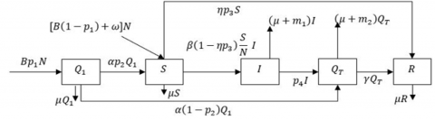
The transfer diagram of the model can be seen in Figure 1 and the meaning of every parameter is given in Table 1. The definition of every variable is given. $S, I$, and $R$ are the number of susceptible, infected, and recovered people respectively. $Q_1$ is the number of quarantined persons from immigration. $Q_T$ is the number of quarantined infected people.
Figure 1. The transfer diagram of the QSIQR model
Table 1. The definition of the parameter in the model
|
Parameter |
Definition |
|
$B$ |
the rate of persons entering the population from immigration |
|
$p_1$ |
the proportion of persons quarantined from immigration |
|
$p_2$ |
the proportion of quarantined persons free from infection |
|
$\omega$ |
the birth rate |
|
$\mu$ |
the natural death rate |
|
$p_3$ |
the vaccination rate of susceptible persons |
|
$\alpha$ |
the rate of persons out of quarantine |
|
$\beta$ |
the infection rate of susceptible persons |
|
$\eta$ |
the effectiveness of vaccination |
|
$m_1, m_2$ |
the death rate because of infection |
|
$p_4$ |
the rate of infected persons who get quarantine and treatments |
|
$\gamma$ |
the recovery rate of the quarantined person |
In this research, we assumed that the birth rate has the same value as the natural death rate, the death rate due to infection of the quarantine-infected group is too small, and all immigration persons must be quarantined.
Kementerian Kesehatan Republik Indonesia [21] stated that the majority of deaths due to COVID-19 in Indonesia occurred in patients with comorbidities, such as heart disease, diabetes, and respiratory disorders, while patients undergoing centralized isolation or quarantine with mild to moderate symptoms showed a very high recovery rate. The death rate of fully vaccinated COVID-19 patients, most of whom were included in the group undergoing centralized quarantine, was only 0.21% [22]. The results of the study by Bi et al. [23] showed that the rate of severe symptoms and death was very low, especially among those who were identified and quarantined early. There were no deaths among close contacts who were quarantined, indicating the effectiveness of quarantine in preventing the severity of infection. Based on these data, it can be concluded that the death rate in the subpopulation quarantined due to infection is very low, so it can be assumed to be zero in mathematical modeling. Meanwhile, the basis for choosing the value $p_1=1$ is the government policies that require everyone who comes from a country or region infected with an infectious disease to undergo health quarantine. The policies can be found in the studies [24-26]. Hence, $\omega=\mu, m_2=0$, and $p_1=1$, then based on Figure 1, we got System (1)
$\begin{gathered}\frac{d Q_1}{d t}=B N-(\alpha+\mu) Q_1 \\ \frac{d S}{d t}=\alpha p_2 Q_1+\mu N-\beta\left(1-\eta p_3\right) \frac{S}{N} I-\left(\mu+\eta p_3\right) S \\ \frac{d I}{d t}=\beta\left(1-\eta p_3\right) \frac{S}{N} I-\left(\mu+m_1+p_4\right) I \\ \frac{d Q_T}{d t}=\alpha\left(1-p_2\right) Q_1+p_4 I-(\mu+\gamma) Q_T \\ \frac{d R}{d t}=\gamma Q_T+\eta p_3 S-\mu R \\ N=Q_1+S+I+Q_T+R\end{gathered}$ (1)
We give the initial condition of every variable in the System (1) such that
$\begin{gathered}Q_1(0) \geq 0, S(0) \geq 0, I(0)>0, Q_T(0) \geq 0 \text { and } R(0) \geq 0\end{gathered}$ (2)
2.2 Parameter estimation and data fitting
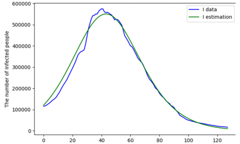
In this subsection, we did parameter estimation and model validation. We used data from many kinds of sources. Data on the population of Indonesia based on the 2020 census was obtained from the reference [27], and we got 270,203,917 persons. We estimate the parameter $B$ using immigration data from the study [28]. We got that the daily average of immigration from September 2020 to October 2021 is 4360.390588 persons. Using the total population of Indonesia based on census in 2020, we got $B=0.00001614$. We got $\mu=0.0000357$ from the study [29] (assuming that the life expectancy of Indonesian people is about 77 years). We used data about the COVID-19 epidemic from the study [30]. We used data about new deaths and newly recovered from June $13^{\text{th}}, 2021$, to October, $19^{\text{th}}, 2021$, and we obtained $m_1=$0.001971553 and $\gamma=0.063230801$. The quarantine period for an immigration person is about 7 to 14 days, so we got the value of $\alpha$ is about $0.07142-0.14286$. Nasir et al. [31] stated that the range of $\eta$ is $62.1 \%-95 \%$. Nasir et al. [31] also stated that the average daily vaccination rate is $50,056-71,050$ doses, so we got the range $p_3$ is 0,0001866 to 0,0002649. We estimated parameter $\beta, p_2$, and $p_4$ using the fourth-order Runge-Kutta Method. We also use data on the number of infected persons from June $13^{\text {th}}$, 2021 to October, $19{ }^{\text {th}}$, 2021 (128 data). We have chosen data from that period because the peak of the outbreak occurred during that period. We got $\beta=$ $0.97, p_2=0.99$, and $p_4=0.9$. We also got MAPE= 0.098667. We used initial values of every parameters, i.e., $Q_{1_0}=139433, I_0=113388, R_0=1745091$ and we assumed that $Q_{T_0}=I_0$ and $S_0=N_0-\left(Q_{1_0}+I_0+Q_{T_0}=\right.$ $\left.R_0\right)$ where $N_0=270,203,917$. A graphic of $I$ data versus $I$ estimation is given in Figure 2. The values of all parameters are given in Table 2.
Figure 2. Graphic I data and I estimation
Table 2. The value of the parameter in the model
|
Parameter |
Value |
Parameter |
Value |
|
B |
0.00001614 |
$\beta$ |
0.97 |
|
$\mu$ |
0.0000357 |
$\eta$ |
0.95 |
|
$\alpha$ |
0.071428571 |
$p_3$ |
0.000263158 |
|
$m_1$ |
0.001971553 |
$p_4$ |
0.9 |
|
$p_2$ |
0.99 |
$\gamma$ |
0.063230801 |
2.3 The membership function of the fuzzy parameter
In this research, we assumed that the humidity is constant. Using the membership function of fuzzy parameters, we defined $\beta$ and $p_4$ as follows:
$\beta(T)=\left\{\begin{array}{c}\beta_{\min }, \quad \text { if } \mathrm{T}<\mathrm{T}_{\min } ; \\ \beta_{min }+\beta_1(1-\pi)(1-\theta) \cdot \frac{\left(\mathrm{T}-\mathrm{T}_{\min }\right)}{\left(\mathrm{T}_{\mathrm{opt}}-\mathrm{T}_{\min }\right)}, \\ \text { if } \mathrm{T}_{\min } \leq \mathrm{T}<\mathrm{T}_{\mathrm{opt}} ; \\ \beta_{min }+\beta_1(1-\pi)(1-\theta) \cdot \frac{\left(\mathrm{T}_{\max }-\mathrm{T}\right)}{\left(\mathrm{T}_{\max }-\mathrm{T}_{\mathrm{opt}}\right)}, \\ \text { if } \mathrm{T}_{\mathrm{opt}} \leq \mathrm{T}<\mathrm{T}_{\max } ; \\ \beta_{min ,} \text { if } \mathrm{T} \geq \mathrm{T}_{\max }\end{array}\right.$ (3)
where,
$\begin{gathered}\beta_{min }+\beta_1(1-\pi)(1-\theta)=1 \Leftrightarrow \beta_{min } =1-\beta_1(1-\pi)(1-\theta),\end{gathered}$
$p_4(\beta)=\left\{\begin{array}{c}p_4^0, \quad \text { if } 0 \leq \beta<\beta_{\min } \\ p_4^0+c \cdot \beta(T), \quad \text { if } \beta_{\min } \leq \beta<\beta\left(T_{ {opt }}\right) \\ 1, \quad \text { if } \beta=\beta\left(T_{ {opt }}\right)\end{array}\right.$
and $\quad p_4^0+c \cdot \beta\left(T_{o p t}\right)=1 \Leftrightarrow p_4^0=1-c\left[\beta_{\min }+\beta_1(1-\right.$ $\pi)(1-\theta)]$. Let $Y_{(\pi, \theta)}=\left[\beta_{\min }+\beta_1(1-\pi)(1-\theta)\right]$. Hence, we get Eq. (4)
$p_4(T)$$=\left\{\begin{array}{c}1-c \cdot Y_{(\pi, \theta),} \quad \text { if } T<T_{min } \\ 1-c \cdot Y_{(\pi, \theta)}\left[1-\frac{\left(T-T_{min }\right)}{\left(T_{o p t}-T_{min }\right)}\right], \text { if } T_{min } \leq T<T_{o p t} \\ 1-c \cdot Y_{(\pi, \theta)}\left[1-\frac{\left(T_{max }-T\right)}{\left(T_{max }-T_{o p t}\right)}\right], \text { if } T_{o p t} \leq T<T_{max } \\ 1-c \cdot Y_{(\pi, \theta),} \quad \text { if } T \geq T_{max }\end{array}\right.$ (4)
where, $\beta_1$ is the standard virus transmission rate (based on the characteristics of the virus), $\pi$ is the proportion of susceptible persons in implementing health protocols, $\theta$ is the effectiveness of government policies like vaccination and quarantine, and $c$ is the weight of $\beta$ for $p_4 \cdot T_{\min }, T_{\text {opt}}$, and $T_{\text {max}}$ successively are minimum, optimum, and maximum temperatures $\left({ }^{\circ} \mathrm{C}\right)$. Anis [18] said that the optimal temperature for the spread of COVID-19 ranges from $13^{\circ} \mathrm{C}$ to $24^{\circ} \mathrm{C}$, where cities with temperatures below $24^{\circ} \mathrm{C}$ are categorized as highrisk areas for transmission. Temperatures between $26^{\circ} \mathrm{C}-30^{\circ} \mathrm{C}$ with humidity above $60 \%$ do not have a significant impact on the spread of COVID-19 [32]. Let $\beta_1=0.99, T_{\min }=4,13 \leq$ $T_{\text {opt }} \leq 24$, and $T_{\text {max }}=26$. Assumed that the value of $\beta=$ 0.97 and $p_4=0.9$ (Table 2) occurred at $T=25, \pi=0.8$ and $\theta=0.698$. Then we get $c=0.2$. The value of $\beta$ and $p_4$ based on $T$ are given in Table 3.
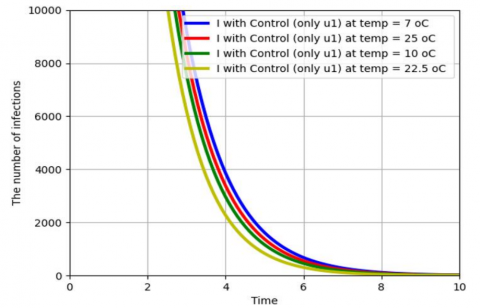
The graphs of I with changing temperature (without control parameter) are given in Figure 3.
From Table 3 and Figure 3, the ratio between the rate of quarantine for infected people and the rate of infection is greater, causing the outbreak to disappear more quickly.
Table 3. The value of $\beta$ and $p_4$ based on $T$ where $\pi=0.8$ and $\theta=0.698$
|
$T$ |
$\boldsymbol{\beta}$ |
$p_4$ |
$\frac{p_4}{\beta}$ |
|
7℃ |
0.960136 |
0.866667 |
0.90265 |
|
10℃ |
0.980068 |
0.933333 |
0.95231 |
|
22.5℃ |
1 |
1 |
1 |
|
25℃ |
0.970102 |
0.9 |
0.92774 |
Figure 3. The graph of I by changing temperature
2.4 Control optimal model
We added two control parameters to System (1), and let $\beta(T)=\hat{\beta}, p_4(T)=\widehat{p_4}$, then we got System (5)
$\begin{gathered}\frac{d Q_1}{d t}=B N-(\alpha+\mu) Q_1 \\ \frac{d S}{d t}=\alpha p_2 Q_1+\mu N-\left(1-u_1\right) \hat{\beta}\left(1-\eta p_3\right) \frac{S}{N} I \\ -\left(\mu+\eta p_3\right) S \\ \frac{d I}{d t}=\left(1-u_1\right) \hat{\beta}\left(1-\eta p_3\right) \frac{S}{N} I-\left(\mu+m_1+\widehat{p_4}+u_2\right) I \\ \frac{d Q_T}{d t}=\alpha\left(1-p_2\right) Q_1+\left(\widehat{p_4}+u_2\right) I-(\mu+\gamma) Q_T \\ \frac{d R}{d t}=\gamma Q_T+\eta p_3 S-\mu R \\ N=Q_1+S+I+Q_T+R\end{gathered}$ (5)
The meaning of two control parameters is:
$u_1$: a policy to prevent the spread of disease among susceptible people
$u_2$: quarantine and treatment efforts to minimize infection or maximize recovery.
Let $U=\left\{\left(u_1(t), u_2(t)\right): 0 \leq u_1<1,0 \leq u_2<1,0<t<\right.$ $\left.t_f\right\}$ is the set of receivable controls.
The goal is to find a control $u$ that produces the lowest value for the objective function $J$ without sacrificing the cost efficiency of implementation in System (5).
Let $J=\min _{u_1, u_2} \int_0^{t_f}\left(I+\frac{1}{2} \sum_{i=1}^2 w_i u_1^2\right) d t$ (6)
Subject to (5) where $w_1$ and $w_2$ are positive constants representing the relative cost weights for implementing control efforts $u_1$ and $u_2$ [15]. We assumed that the costs were nonlinear. Therefore, the control variables in the objective function $J$ are in the form of second-degree polynomials [33, 34]. Our main objective is to minimize the number of people exposed and affected by the disease while keeping the control costs as low as possible. Thus, we are going to find optimal controls $\left(u_1^*, u_2^*\right)$, such that
$J\left(u_1^*, u_2^*\right)=\min \left\{J\left(u_1, u_2\right) \mid\left(u_1, u_2\right) \in U\right\}$
where, $u_1$ and $u_2$ are measurable with $0 \leq u_i<1, i=1,2$ for $t \in\left[0, t_f\right]$.
3.1 The Hamiltonian and optimality system
Here, we can formulate the necessary conditions for applying the Pontryagin Maximum Principle to obtain the optimal solution [12]. Therefore, this principle converts the model Eqs. (5), and (6) into a problem of minimizing a Hamiltonian, $H$, pointwise concerning $u_1$ and $u_2$, and we obtained a Hamiltonian $(H)$ defined as:
$H(t, x(t), u(t), \lambda(t))=f(t, x(t), u(t))+\lambda g(t, x(t), u(t))$
where,
$\begin{aligned} & f(t, x(t), u(t))=I+\frac{1}{2} w_1 u_1^2+\frac{1}{2} w_2 u_2^2 ,\\ & g(t, x(t), u(t))=\left(g_1, g_2, g_3, g_4, g_5, g_6\right)^T\end{aligned}$,
and
$\begin{gathered}g_1=B N-(\alpha+\mu) Q_1 \\ g_2=\alpha p_2 Q_1+\mu N-\left(1-u_1\right) \hat{\beta}\left(1-\eta p_3\right) \frac{S}{N} I-\left(\mu+\eta p_3\right) S \\ g_3=\left(1-u_1\right) \hat{\beta}\left(1-\eta p_3\right) \frac{S}{N} I-\left(\mu+m_1+\widehat{p_4}+u_2\right) I \\ g_4=\alpha\left(1-p_2\right) Q_1+\left(\widehat{p_4}+u_2\right) I-(\mu+\gamma) Q_T \\ g_5=\gamma Q_T+\eta p_3 S-\mu R\end{gathered}$
where,
$N=Q_1+S+I+Q_T+R$
Hence the Hamiltonian becomes $Q_1(0) \geq 0, S(0) \geq$ $0, I(0)>0, Q_T(0) \geq 0$, and $R(0) \geq 0$.
$\begin{gathered}H\left(t, Q_1, S, I, Q_T, R\right)=f\left(t, I, u_1, u_2\right)+\lambda_1 \frac{d Q_1}{d t} +\lambda_2 \frac{d S}{d t}+\lambda_3 \frac{d I}{d t}+\lambda_4 \frac{d Q_T}{d t}+\lambda_5 \frac{d R}{d t} \\ H=I+\frac{1}{2} w_1 u_1^2+\frac{1}{2} w_2 u_2^2+\lambda_1 g_1 +\lambda_2 g_2+\lambda_3 g_3+\lambda_4 g_4+\lambda_5 g_5\end{gathered}$
where, $\lambda_i, i=1,2, \ldots, 5$ are adjoint variables with transversality conditions $\lambda_i\left(t_f\right)=0, i=1,2, \ldots, 5$ for an optimal control $\left(u_1^*, u_2^*\right)$ that minimizes $J\left(u_1, u_2\right)$ and
$\frac{d \lambda}{d t}=-\frac{\partial H}{\partial X}$
where, $X=\left(Q_1, S, I, Q_T, R\right)^T$ and $\lambda=\left(\lambda_1, \lambda_2, \lambda_3, \lambda_4, \lambda_5\right)^T$, $\lambda\left(t_f\right)=0$ transcendentality condition.
Hence
$\begin{gathered}\frac{d \lambda_1}{d t}=-\frac{\partial H}{\partial Q_1}=-\lambda_1[B-(\alpha+\mu)]+\left(\lambda_3-\lambda_2\right)\left(1-u_1\right) \\ \hat{\beta}\left(1-\eta p_3\right) \frac{S I}{N^2}-\lambda_2\left(\alpha p_2+\mu\right)-\lambda_4 \alpha\left(1-p_2\right) \\ \frac{d \lambda_2}{d t}=-\frac{\partial H}{\partial S}=-\lambda_1 B-\left(\lambda_3-\lambda_2\right)\left(1-u_1\right) \\ \hat{\beta}\left(1-\eta p_3\right) \frac{I\left(Q_1+I+Q_T+R\right)}{N^2}+\lambda_2 \eta p_3-\lambda_5 \eta p_3 \\ \frac{d \lambda_3}{d t}=-\frac{\partial H}{\partial I}=-1-\lambda_1 B-\lambda_2 \mu \\ -\left(\lambda_3-\lambda_2\right)\left(1-u_1\right) \hat{\beta}\left(1-\eta p_3\right) \frac{S\left(Q_1+S+Q_T+R\right)}{N^2} \\ +\lambda_3\left(\mu+m_1+\widehat{p_4}+u_2\right)-\lambda_4\left(\widehat{p_4}+u_2\right) \\ \frac{d \lambda_4}{d t}=-\frac{\partial H}{\partial Q_T}=-\lambda_1 B-\lambda_2 \mu+\left(\lambda_3-\lambda_2\right)\left(1-u_1\right) \\ \hat{\beta}\left(1-\eta p_3\right) \frac{S I}{N^2}+\lambda_4(\mu+\gamma)-\lambda_5 \gamma \\ \frac{d \lambda_5}{d t}=-\frac{\partial H}{\partial R}=-\lambda_1 B-\lambda_2 \mu+\left(\lambda_3-\lambda_2\right)\left(1-u_1\right) \\ \hat{\beta}\left(1-\eta p_3\right) \frac{S I}{N^2}+\lambda_5 \mu\end{gathered}$ (7)
Similarly, we obtained the controls by solving the equation $\frac{\partial H}{\partial u_1}=0$ at $u_i^*$, for $i=1,2$ following Pontryagin's methods and obtained:
$\begin{gathered}\frac{\partial H}{\partial u_1}=0 \Leftrightarrow u_1=\frac{\left(\lambda_3-\lambda_2\right) \hat{\beta}\left(1-\eta p_3\right)}{w_1} \frac{S I}{N} \\ \frac{\partial H}{\partial u_2}=0 \Leftrightarrow u_2=\frac{\left(\lambda_3-\lambda_4\right)}{w_2} I\end{gathered}$
Hence,
$\begin{aligned} u_1^*= & \max \left\{0, \min \left\{1, \frac{\left(\lambda_3-\lambda_2\right) \beta\left(1-\eta p_3\right)}{w_1} \frac{S I}{N}\right\}\right\} =\left\{\begin{array}{c}0, \frac{\left(\lambda_3-\lambda_2\right) \hat{\beta}\left(1-\eta p_3\right)}{w_1} \frac{S I}{N} \leq 0 \\ \frac{\left(\lambda_3-\lambda_2\right) \hat{\beta}\left(1-\eta p_3\right)}{w_1} \frac{S I}{N}, \\ 0<\frac{\left(\lambda_3-\lambda_2\right) \hat{\beta}\left(1-\eta p_3\right)}{w_1} \frac{S I}{N}<1 \\ 1, \frac{\left(\lambda_3-\lambda_2\right) \beta\left(1-\eta p_3\right)}{w_1} \frac{S I}{N} \geq 1\end{array}\right.\end{aligned}$ (8)
$\begin{aligned} u_2^*=\max & \left\{0, \min \left\{1, \frac{\left(\lambda_3-\lambda_4\right)}{w_2} I\right\}\right\} =\left\{\begin{array}{c}0, \frac{\left(\lambda_3-\lambda_4\right)}{w_2} I \leq 0 \\ \frac{\left(\lambda_3-\lambda_4\right)}{w_2} I, 0<\frac{\left(\lambda_3-\lambda_4\right)}{w_2} I<1 \\ 1, \frac{\left(\lambda_3-\lambda_4\right)}{w_2} I \geq 1\end{array}\right.\end{aligned}$ (9)
3.2 Numerical simulation
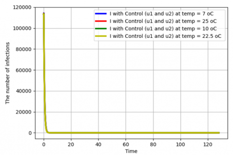
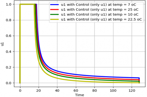
We use the parameter value in Table 1 for simulation. We use the following data to calculate the values of $w_1$ and $w_2$. The total cost for handling the COVID-19 outbreak is IDR 1895.5 trillion [35]. The total cost of vaccination is IDR 57.84 trillion [36] and counseling is IDR 0.75 trillion [37], so the total cost for vaccination and counseling is IDR 58.59 trillion. Hence, we get $w_1=\frac{58.59}{1895.5} \approx 0.03$. The total cost of quarantine and treatment in 2020 is IDR 62.7 trillion [38], in 2021 and 2022 respectively IDR 100 trillion and IDR 122.5 trillion [39], so the total cost for quarantine and treatment is IDR 285.2 trillion. Hence, we get $w_2=0.15$. Based on Rois et al. [15], we take three strategies, i.e., Strategy 1 uses only $u_1$, Strategy 2 uses only $u_2$, and Strategy 3 uses both $u_1$ and $u_2$. The simulation graphics of the optimal control problem related to temperature changes can be seen in Figure 4.
Figures 4 (b) and (d) show that if only a single control action (only $u_1$ or $u_2$) is applied, then the number of infected people becomes zero starting at day 8 for every temperature. Figure 4(f) shows that if both control actions $\left(u_1\right.$ and $\left.u_2\right)$ are applied, then the number of infected people becomes zero starting at day 4 for every temperature. Hence, the application of both control actions ($u_1$ and $u_2$) caused the epidemic will be extinct faster than the effect of the application of a single control action.
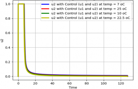
From Figures 4(g) and 4(h), we see that to minimize the objective function $J$ in (4), the value of $u_1$ and $u_2$ (only one of them is applied) are maintained at the maximum level of $100 \%$ for about 19 days and 17 days respectively before relaxing to the minimum in final time. As expected, the number of infected people is reduced when control is applied. Further, in Figures 4(i) and 4(j) the value of $u_1$ and $u_2$ (both are applied) are maintained at the maximum level of $100 \%$ for about 10 days and 7 days, respectively before relaxing to the minimum in final time. Hence, the application of both control actions will shorten the duration of the maximum level of every control action. Hence, the application of the two control actions is significantly more effective in preventing the spread of the infection than when only a single control is applied. Information about confidence interval of $I$ can be seen in Table 4.
(a) The infected numbers with control only $u_1$
(b) The infected numbers with control only $u_1$ (zoom version)
(c) The infected numbers with control only $u_2$
(d) The infected numbers with control only $u_2$ (zoom version)
(e) The infected numbers with control $u_1$ and $u_2$
(f) The infected numbers with control $u_1$ and $u_2$ (zoom version)
(g) Profile of $u_1$ (only $u_1$)
(h) Profile of $u_2$ (only $u_2$ )
(i) Profile of $u_1$ (both non-zero)
(j) Profile of $u_2$ (both non-zero)
Figure 4. The graphics of the simulation at temperature 7℃, 10℃, 22.5℃, and 25℃
Table 4. Confidence interval of $I$
|
Temp. (℃) |
Control Options |
Mean |
Std. Dev. |
95% CI Lower |
95% CI Upper |
|
7 |
no control |
377564.6364 |
354948.8208 |
358119.5963 |
397009.6765 |
|
only u1 |
1073.6478 |
7933.5812 |
639.0251 |
1508.2704 |
|
|
only u2 |
1019.7155 |
7745.0977 |
595.4184 |
1444.0125 |
|
|
u1 and u2 |
524.0944 |
5701.2965 |
211.7622 |
836.4266 |
|
|
10 |
no control |
143560.9293 |
81991.6163 |
139069.2106 |
148052.6481 |
|
only u1 |
995.7220 |
7639.4728 |
577.2114 |
1414.2326 |
|
|
only u2 |
967.7934 |
7539.2015 |
554.7759 |
1380.8109 |
|
|
u1 and u2 |
505.3025 |
5594.2811 |
198.8329 |
811.7721 |
|
|
22.5 |
no control |
34944.7091 |
35018.8495 |
33026.2834 |
36863.1348 |
|
only u1 |
928.1639 |
7374.3248 |
524.1788 |
1332.1491 |
|
|
only u2 |
920.6920 |
7347.1677 |
518.1946 |
1323.1894 |
|
|
u1 and u2 |
487.7614 |
5492.4407 |
186.8709 |
788.6519 |
|
|
25 |
no control |
251510.8476 |
183987.2562 |
241431.5365 |
261590.1587 |
|
only u1 |
1033.2452 |
7782.5808 |
606.8948 |
1459.5957 |
|
|
only u2 |
993.1068 |
7640.3117 |
574.5502 |
1411.6634 |
|
|
u1 and u2 |
514.5339 |
5647.1140 |
205.1700 |
823.8978 |
3.3 Cost-effectiveness analysis
Cost-effectiveness analysis is used to determine which COVID-19 control measures are most effective and efficient, either by a single application or a combination of two given measures. The goal is to optimally reduce the spread of COVID-19 at the lowest possible cost. Hence, we used the incremental cost-effectiveness ratio (ICER) to determine the most effective optimal control measure, and the ICER formula is given by
$\mathrm{ICER}=\frac{T C}{T N}$ (10)
where, $T C$ is the change in total costs between control measures and $T N$ is the change in the total number of infections averted by control measures [40].
The total cost is obtained from the objective function (6), and the total number of infections averted is obtained by calculating the difference between infectious individuals without and with control measures. Let S1, S2, and S3 represent Strategy 1, Strategy 2, and Strategy 3, respectively. The results of the ICER calculation of each Strategy by using Eq. (10) are given in Table 5.
From Table 5, we see that ICER(S1) is less than ICER(S2) for every temperature. This means that Strategy 2 is more costly and less effective than Strategy 1. In other words, Strategy 1 dominates Strategy 2. Thus, a single implementation of $u_2$ control is removed from the list. Therefore, ICER (S1) and ICER (S3) are calculated again in Table 6.
Table 5. ICER calculation of every Strategy at different temperatures
|
Temp. |
Control Measure |
Total Infections Prevented |
Total Costs |
ICER |
|
7℃ |
S1 |
481908465 |
107925.2121 |
0.000223954 |
|
S2 |
481977499 |
136194.3264 |
0.409499455 |
|
|
S3 |
482611894 |
72754.2135 |
-0.100000972 |
|
|
10℃ |
S1 |
182483465 |
101735.2461 |
0.000557504 |
|
S2 |
182519214 |
129548.1752 |
0.778013404 |
|
|
S3 |
183111202 |
70348.8096 |
-0.100000904 |
|
|
22.5℃ |
S1 |
43541178 |
96288.8787 |
0.002211444 |
|
S2 |
43550742 |
123519.1158 |
2.847137673 |
|
|
S3 |
44104893 |
68103.5239 |
-0.100000865 |
|
|
25℃ |
S1 |
320611331 |
104727.5580 |
0.000326650 |
|
S2 |
320662708 |
132788.3466 |
0.546171509 |
|
|
S3 |
321275282 |
71530.4446 |
-0.100000934 |
Table 6. ICER calculation of Strategy 1 and Strategy 3 at different temperatures
|
Temp. |
Control Measure |
Total Infections Prevented |
Total Costs |
ICER |
|
7℃ |
S1 |
481908465 |
107925.2121 |
0.0002240 |
|
S3 |
482611894 |
72754.2135 |
-0.0499994 |
|
|
10℃ |
S1 |
182483465 |
101735.2461 |
0.0005575 |
|
S3 |
183111202 |
70348.8096 |
-0.0499993 |
|
|
22.5℃ |
S1 |
43541178 |
96288.8787 |
0.0022114 |
|
S3 |
44104893 |
68103.5239 |
-0.0499993 |
|
|
25℃ |
S1 |
320611331 |
104727.5580 |
0.0003266 |
|
S3 |
321275282 |
71530.4446 |
-0.0499994 |
From Table 6, we see that Strategy 3 dominates Strategy 1 since ICER(S3) is less than ICER(S1). This means Strategy 3 is less costly and more effective than Strategy 1. Hence, a single implementation of preventive measures is excluded from the list. Hence, the application of the two control actions is significantly more cost-effective than when only a single control is applied.
This result is similar to the result obtained by Rois et al. [12], namely, Strategy 3 (combined controls) is more cost-effective than single controls. The added value of this study is that the optimal control analysis is carried out at several different temperature conditions, and also the process of determining the weight value for each control action is also given.
Using Pontryagin’s maximum principle, the application of the two control actions at every temperature is significantly more effective in preventing the spread of the infection than when only a single control is applied. From the result of the Cost-effectiveness analysis, the application of the two control actions at every temperature is significantly more cost-effective than when only a single control is applied.
This study still has several limitations, one of which is the lack of empirical data on the relationship between temperature and transmission rate used in validating the fuzzy parameter formulation. Another limitation is that data on the total cost of implementing control measures cannot yet be obtained from scientific journal article sources. The results of this study can be used as one of the supporters of policy making in dealing with future outbreaks that have similar behavior to the COVID-19 outbreak.
This research was supported by the Education Fund Management Institution (Lembaga Pengelola Dana Pendidikan/LPDP) and the Center for Higher Education Funding and Assessment (Pusat Pembiayaan dan Asesmen Pendidikan Tinggi/PPAPT) from the Indonesian Education Scholarship Program (Beasiswa Pendidikan Indonesia/BPI), Ministry of Higher Education, Science, and Technology of the Republic of Indonesia.
[1] Aeni, N. (2021). Pandemi COVID-19: Dampak kesehatan, ekonomi, & sosial. Jurnal Litbang: Media Informasi Penelitian, Pengembangan Dan IPTEK, 17(1): 17-34. https://doi.org/10.33658/jl.v17i1.249
[2] Rehman, S., Nnabuike, U.E., Abbas, A., Rahman, A., Malik, U., Effendi, M.H., Hussain, K., Raza, M.A. (2022). A study on the Impacts of COVID-19 on health, economy, employment and social life of people in Indonesia. Advancements in Life Sciences, 9(3): 340-346. http://doi.org/10.62940/als.v9i3.1509
[3] Tambunan, N., Fauziyah, S. (2023). Analisis dampak pandemi COVID 19 terhadap perekonomian di Indonesia. Jurnal Ilmiah Wahana Pendidikan, 9(22): 719-726. https://doi.org/10.5281/zenodo.10134216
[4] Yogadhita, G.Y., Donna, B., Ariani, M., Aktariyani, T., Pangaribuan, H.R. (2021). Dampak Pembatasan sosial berskala besar di komunitas terhadap kunjungan pasien COVID-19 di Rumah Sakit. Jurnal Kebijakan Kesehatan Indonesia: JKKI, 10(1): 8-16. https://doi.org/10.22146/jkki.61660
[5] Nanda, I.Y., Yahya, M.R., Yuwono, T. (2023). Analisis pengaruh kebijakan pembatasan sosial berskala besar terhadap partisipasi masyarakat di Kabupaten Kampar. NeoRespublica: Jurnal Ilmu Pemerintahan, 5(1): 285-297. https://doi.org/10.52423/neores.v5i1.168
[6] Muhandari, F., Ilham, M. (2021). Efektivitas kebijakan pemberlakuan pembatasan kegiatan masyarakat dalam rangka pengendalian penyebaran COVID-19 di Kota Bandung. Jurnal Ilmiah Administrasi Pemerintahan Daerah, 13(2): 42-51. https://doi.org/10.33701/jiapd.v13i2.2244
[7] Rois, M.A., Alfiniyah, C., Martini, S., Aldila, D., Nyabadza, F. (2024). Modeling and optimal control of COVID-19 with comorbidity and three-dose vaccination in Indonesia. Journal of Biosafety and Biosecurity, 6(3): 181-195. https://doi.org/10.1016/j.jobb.2024.06.004
[8] Yong, B., Hoseana, J., Owen, L. (2022). From pandemic to a new normal: Strategies to optimise governmental interventions in Indonesia based on an SVEIQHR-type mathematical model. Infectious Disease Modelling, 7(3): 346-363. https://doi.org/10.1016/j.idm.2022.06.004
[9] Azzahra, N.F. (2021). Kontrol optimal penyebaran COVID-19 model SEIR di Jakarta. ITS Repository, 11(2). https://doi.org/10.12962/j23373520.v11i2.76998
[10] Nasution, N.N., Sinaga, L.P. (2021). Analisis sensitivitas dan kontrol optimal model seir penyebaran COVID-19. Karismatika, 7(3): 25-40. https://doi.org/10.24114/jmk.v7i3.32461
[11] Liu, H., Tian, X. (2020). Data-driven optimal control of a SEIR model for COVID-19. arXiv Preprint arXiv:2012.00698. https://doi.org/10.48550/arXiv.2012.00698
[12] Rois, M.A., Trisilowati, H.U. (2021). Optimal control of mathematical model for COVID-19 with quarantine and isolation. International Journal of Engineering Trends and Technology, 69(6): 154-160. https://doi.org/10.14445/22315381/IJETT-V69I6P223
[13] Tiwari, A. (2020). Modelling and analysis of COVID-19 epidemic in India. Journal of Safety Science and Resilience, 1(2): 135-140. https://doi.org/10.1016/j.jnlssr.2020.11.005
[14] Abdy, M., Side, S., Annas, S., Nur, W., Sanusi, W. (2021). An SIR epidemic model for COVID-19 spread with fuzzy parameter: The case of Indonesia. Advances in Difference Equations, 2021: 1-17. https://doi.org/10.1186/s13662-021-03263-6
[15] Rois, M.A., Fatmawati, Alfiniyah, C., Chukwu, C.W. (2023). Dynamic analysis and optimal control of COVID-19 with comorbidity: A modeling study of Indonesia. Frontiers in Applied Mathematics and Statistics, 8: 1096141. https://doi.org/10.3389/fams.2022.1096141
[16] Tosepu, R., Gunawan, J., Effendy, D.S., Ahmad, L.O.A.I., Lestari, H., Bahar, H., Asfian, P. (2020). Correlation between weather and COVID-19 pandemic in Jakarta, Indonesia. Science of the Total Environment, 725: 138436. https://doi.org/10.1016/j.scitotenv.2020.138436
[17] Wang, J.Y., Tang, K., Feng, K., Lin, X., Lv, W.F., Chen, K., Wang, F. (2021). Impact of temperature and relative humidity on the transmission of COVID-19: A modelling study in China and the United States. BMJ Open, 11(2): e043863. https://doi.org/10.1136/bmjopen-2020-043863
[18] Anis, A. (2020). The effect of temperature upon transmission of COVID-19 Australia and Egypt case study. SSRN, 3567639: 1-20. https://doi.org/10.2139/ssrn.3567639
[19] Fang, Z.G., Yang, S.Q., Lv, C.X., An, S.Y., Guan, P., Huang, D.S., Zhou, B.S., Wu, W. (2022). The correlation between temperature and the incidence of COVID-19 in four first-tier cities of China: A time series study. Environmental Science and Pollution Research, 29(27): 41534-41543. https://doi.org/10.1007/s11356-021-18382-6
[20] Rois, M.A., Fatmawati, A.C. (2023). Mathematical modeling of COVID-19 with partial comorbid subpopulations and two isolation treatments in Indonesia. International Journal of Mathematics and Computer Science, 18: 233-242.
[21] Kementerian Kesehatan Republik Indonesia. (2021). Komorbid Jadi Penyebab Terbanyak Kematian Pasien COVID-19.
[22] Kompas. (2021). Luhut: Angka kematian pasien COVID-19 yang Sudah Divaksin Sangat Rendah, 0,21%.
[23] Bi, Q.F., Wu, Y.S., Mei, S.J., Ye, C.F., Zou, X., Zhang, Z., et al. (2020). Epidemiology and transmission of COVID-19 in 391 cases and 1286 of their close contacts in Shenzhen, China: A retrospective cohort study. The Lancet Infectious Diseases, 20(8): 911-919. https://doi.org/10.1016/S1473-3099(20)30287-5
[24] Pemerintah Pusat Indonesia. (2018). Undang-undang (UU) Nomor 6 Tahun 2018 tentang Kekarantinaan Kesehatan. https://peraturan.bpk.go.id/Details/90037/uu-no-6-tahun-2018, accessed on Apr. 12, 2025.
[25] Pemerintah Pusat Indonesia. (2020). Peraturan Pemerintah (PP) Nomor 21 Tahun 2020 tentang Pembatasan Sosial Berskala Besar (PSBB). https://peraturan.bpk.go.id/Details/135059/pp-no-21-tahun-2020, accessed on Apr. 12, 2025.
[26] Satuan Tugas (Satgas) Penanganan COVID-19. (2022). Surat Edaran (SE) Nomor 15 Tahun 2022 tentang Protokol Kesehatan Perjalanan Luar Negeri pada Masa Pandemi Corona Virus Disease 2019 (COVID-19).
[27] Badan Pusat Statistik. (2020). Jumlah Penduduk menurut Wilayah dan Jenis Kelamin, INDONESIA, Tahun 2020. https://sensus.bps.go.id/topik/tabular/sp2020/1/1/0, accessed on Sep. 2, 2023.
[28] Badan Pusat Statistik. (2021). Jumlah Kunjungan Wisatawan Mancanegara per bulan Menurut Kebangsaan (Kunjungan). https://www.bps.go.id/id/statistics-table/2/MTQ3MCMy/jumlah-kunjungan-wisatawan-mancanegara-per-bulan-menurut-kebangsaan.html.
[29] Resmawan, R., Nuha, A.R., Yahya, L. (2021). Analisis dinamik model transmisi COVID-19 dengan melibatkan intervensi karantina. Jambura Journal of Mathematics, 3(1): 66-79. https://doi.org/10.34312/jjom.v3i1.8699
[30] Hendratno. (2022). COVID-19 Indonesia Dataset. https://www.kaggle.com/datasets/Hendratno/COVID19-indonesia.
[31] Nasir, N.M., Joyosemito, I.S., Boerman, B., Ismaniah, I. (2021). Kebijakan vaksinasi COVID-19: Pendekatan pemodelan matematika dinamis pada efektivitas dan dampak vaksin di Indonesia. Jurnal Pengabdian kepada Masyarakat UBJ, 4(2): 191-204. https://doi.org/10.31599/jabdimas.v4i2.662
[32] Ansari Saleh, A., MA, E.S., Samirah, A.Z., Rusli, R., Abdul, R. (2021). Association between temperature and relative humidity in relation to COVID-19. Intelligent Automation & Soft Computing, 30(3): 795-803. https://doi.org/10.32604/iasc.2021.016868
[33] Tilahun, G.T., Makinde, O.D., Malonza, D. (2017). Modelling and optimal control of pneumonia disease with cost-effective strategies. Journal of Biological Dynamics, 11(sup2): 400-426. https://doi.org/10.1080/17513758.2017.1337245
[34] Swai, M.C., Shaban, N., Marijani, T. (2021). Optimal control in two strain pneumonia transmission dynamics. Journal of Applied Mathematics, 2021(1): 8835918. https://doi.org/10.1155/2021/8835918
[35] Elena, M. (2022). Airlangga: Total Anggaran Penanganan COVID-19 RI Rp1.895,5 Triliun. https://ekonomi.bisnis.com/read/20220606/9/1540281/airlangga-total-anggaran-penanganan-COVID-19-ri-rp18955-triliun.
[36] Kemenkeu. (2021). Pemerintah Perkuat Program Penanganan Kesehatan untuk Merespon Peningkatan Kasus COVID-19. https://www.menpan.go.id/site/berita-terkini/pemerintah-perkuat-program-penanganan-kesehatan-untuk-merespon-peningkatan-kasus-COVID-19.
[37] TEMPO.CO. (2021). Sri Mulyani Rinci Tambahan Anggaran Kesehatan Pandemi COVID-19 Rp 214 Triliun. https://www.tempo.co/ekonomi/sri-mulyani-rinci-tambahan-anggaran-kesehatan-pandemi-COVID-19-rp-214-triliun-493412.
[38] FIN.CO.ID. (2021). Biaya Pengobatan dan Perawatan Pasien COVID-19 di 2020 Capai Rp62,7 Triliun. https://fin.co.id/2021/09/08/biaya-pengobatan-dan-perawatan-pasien-COVID-19-di-2020-capai-rp627-triliun#gsc.tab=0.
[39] Said, A.A. (2022). Biaya Perawatan Pasien COVID-19 Tembus Rp 100 T pada 2021. https://katadata.co.id/finansial/makro/622f170fb6c89/biaya-perawatan-pasien-COVID-19-tembus-rp-100-t-pada-2021.
[40] Olaniyi, S., Obabiyi, O.S., Okosun, K.O., Oladipo, A.T., Adewale, S.O. (2020). Mathematical modelling and optimal cost-effective control of COVID-19 transmission dynamics. The European Physical Journal Plus, 135(11): 938. https://doi.org/10.1140/epjp/s13360-020-00954-z