Tariq Emad Ali*![]() | Csaba Biro
| Csaba Biro![]() | Alwahab Dhulfiqar Zoltán
| Alwahab Dhulfiqar Zoltán![]()
© 2025 The authors. This article is published by IIETA and is licensed under the CC BY 4.0 license (http://creativecommons.org/licenses/by/4.0/).
OPEN ACCESS
Addressing a variety of networking issues, such as distribution optimization and system provisioning, requires accurate flow pattern estimation. This activity depends on link load proportions in standard IP networks, but the accuracy is frequently harmed since the linear equations driving the traffic estimate process are so poorly understood. Measurements of various flow types are made possible by software-defined networking (SDN), which opens up new alternatives for solving this issue. In order to gather traffic statistics, SDN controllers can also dynamically configure flow entries in the routers' flow tables. The restricted capacity of flow tables, which are usually constructed using expensive ternary content-addressable memory (TCAM) and only provide a certain number of entries for traffic measurement, is a significant drawback. In this study, we offer a new framework for SDN-based IP networks that uses Flow Volume estimates (FVESDN). Our method's capacity to deliberately add flows to the flow tables of SDN routers, so raising the rate of the underlying equations governing Flow Volume estimates, is one of its most notable features. This greatly improves the effectiveness of using TCAMs for traffic measurement. Our thorough performance analysis shows that the suggested framework outperforms current techniques by a significant margin, providing a more potent response to the difficulties presented by FVESDN situations.
SDN, TCAM, TMESDN, flow table, controller, OpenFlow
Flow Volume (FV) is fundamental to addressing numerous network challenges, like traffic-engineering (TE), system provisioning, and crowding managing. However, accurately estimating a network's FV remains a challenging task [1]. The FV, denoted as FV=tlfsd, where, tlfsd is the traffic load drift from source (s) to destination (d) to estimate the load for each pair. In vector v form, this can be expressed as v=[v1, v2, ..., v|z|]FV, where, z is all source-destination (sd) flows, and each section vi corresponds to one FVsd. In traditional internet protocol (IP) networks, Flow Volume Estimation (FVE) relies on link load measurements collected via protocols. Let the route of the link load (LL) represent by $L L^{R V}=$ $\left[L L_1^{R V}, L L_2^{R V}, \ldots, L L_{|s l|}^{R V}\right]$, where, (sl) is the established of links, and $\mathrm{LL}_i^x$ indicates the link load on the link i. The relationship between the traffic flows v and the link loads LLRV is governed by Eq. (1):
$R V \times v=L L^{R V}$ (1)
where, RV is the routing volume indicating whether a flow passes through a particular link [2]. While RV is known and LLRV can be measured, solving for v is problematic because the system of equations is highly under-determined, leading to multiple possible solutions [3]. Although various techniques have been proposed to improve FVE, their accuracy remains limited [4]. The advent of software-defined networking (SDN) introduces new possibilities for addressing this challenge. By separating the data plane and control plane, SDN enabled routers use flow tables (FT) for forwarding, where each entry consists of three parts: A match field (defining the flow), an action field (specifying the routing strategy), and a counter (measuring traffic statistics) [5]. These counters provide additional insights beyond conventional link load measurements. Moreover, SDN controllers can dynamically install flow rules in FT to collect targeted traffic measurements without routing actions. However, this approach faces a key limitation: FT, built using expensive ternary content-addressable memory (TCAM) has limited capacity [6]. Efficiently utilizing this limited TCAM space for traffic measurements is a significant challenge, as excessive usage can impact network resources and operations [7].
This paper presents a novel framework for Flow Volume Estimation SDN (FVESDN) for programming systems. If a flow does not contribute additional information, its inclusion is avoided, optimizing TCAM utilization. The suggested method is versatile and appropriate to various programming system settings. To illustrate its benefits, we evaluate its performance in a hybrid network scenario, where SDN routers coexist with traditional routers, a setup reflecting the gradual adoption of SDN technology in real-world networks. The key contributions of this paper are:
The rest of this paper is structured as follows: Section 2 reviews associated studies on FVE. Section 3 outlines the illustration of the proposed framework and the principles behind the proposed framework. Section 4 proposes methodology for FVE, while Section 5 introduces heuristic algorithms for generating s. Section 6 presents performance evaluation results, and Section 7 presents the scalability and adaptability to dynamic traffic Conditions. Section 8 concludes the paper.
Traditional methods for FVE, like those relying on SNMP measurements, have primarily focused on link loads. One well-known example is the gravity model, as explored in previous studies [8-10]. This method estimates FV by using the total inbound and outbound traffic for each network node, essentially calculating individual flow terms based on the row and column sums of the FV. While it provides a good starting point, its accuracy is limited because it uses sparse and incomplete data. Later, the tomogravity model, introduced in the study [11], improved on this by incorporating link load data, which resulted in better accuracy. Even though these models aren’t perfect, they’ve served as useful tools for providing initial estimates of sd flows something we plan to build upon in our approach. Now, compared to these traditional networks, programmable networks like SDN offer far richer measurement capabilities. These go beyond simple link loads or node-level ingress and egress traffic. Instead, they give much more granular, flow-level insights. This extra information significantly improves the accuracy of FVE techniques designed specifically for these kinds of networks. Broadly speaking, such techniques revolve around three main factors:
One notable method is OpenFV, proposed in the paper [12], which aims to measure all sd flows in the FV. It relies on a centralized controller to identify the routing path for each flow and selects a node along that path to take the measurement. Strategies like round-robin or choosing the least-loaded node are often used here. While this approach works, it struggles with scalability due to the sheer number of flows and the limited size of the TCAM, making it impractical for large-scale networks. To address this, newer approaches like those in these studies [13, 14] have focused on measuring only a subset of sd flows. These methods combine these selected flow measurements with aggregated flow data and existing link load statistics, which are usually gathered using SDN-FT or SNMP. Since only a small number of sd flows are measured, choosing the right flows becomes crucial. Some strategies, such as those discussed in these studies [15, 16], prioritize flows based on their size, which typically requires an initial size estimation. For example, iSTAMP, introduced in the research [15], uses intelligent sampling to estimate flow sizes, though this comes at a high cost in terms of resources. The study [13] suggests two different approaches: Multi-Level Reciprocal Feedback model (MLRF), which breaks down aggregated flows into smaller, more manageable flows until enough data is available to solve the underlying linear equations, which uses preliminary size estimates to prioritize flows for measurement. Both rely on integer programming to determine which nodes should measure the selected flows. OpenMeasure, reported in the research [15], adds a layer of sophistication by applying available knowledge procedures to classify the major drifts and then optimizing their placement using integer programming.
Another approach introduced in the study [17] uses a metric called “flow spread” to prioritize which sd flows to measure. Flow spread represents the range of potential solutions for a given flow in the FV equations, with larger spreads taking priority. However, this method has a key limitation: Selecting one sd flow for measurement can alter the flow spreads of others, meaning recalibration is needed after each selection. One recurring issue in these methods is that they sometimes choose sd flows that don’t add any new information about the FV. This happens when the traffic load of a selected flow can already be inferred from existing measurements. In mathematical terms, such flows don’t growth the rate of the structure of direct calculations used for FVE. Previous studies, like these studies [18, 19], have explored rate-related issues in other areas, such as node placement and packet loss estimation in cloud networks. In this paper, we extend those insights to FVE, ensuring that each selected sd flow contributes meaningful new information by increasing the rate of the equations. This approach not only improves how efficiently the TCAM is used but also boosts the overall accuracy of FVE techniques.
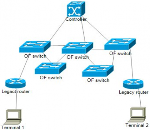
In this study, we focus on a hybrid network configuration, as illustrated in Figure 1, where conventional routers coexist with programmable routers (Hybrid-SDN switches) under the management of an SDN controller. Conventional routers operate using static routing protocols, primarily relying on shortest-path routing to determine the most efficient path for data transmission [13]. In contrast, Hybrid-SDN switches introduce programmability, enabling dynamic traffic management and policy-based routing. The SDN controller centrally manages the Hybrid-SDN switches by installing forwarding rules based on network conditions, security policies, or traffic optimization strategies [16]. This architecture allows us to analyze how SDN-based routing can enhance network performance compared to traditional shortest-path routing. By integrating both conventional and programmable network elements, we evaluate the impact of SDN adoption on key performance metrics such as latency, throughput, and security enforcement. Our study explores various traffic scenarios within this hybrid framework to determine the benefits and challenges associated with SDN integration. The results provide insights into how SDN enhances network adaptability while coexisting with legacy routing mechanisms.
Figure 1. Hybrid SDN environment
We analyze three categories of flow sizes in a hybrid system setup:
These measurements enable the estimation of the network's FV. While LL and DBFs measurements are fixed, the sd flow measurement requires selection, which forms the core of our study. For simplicity, unless stated otherwise, the term, flow, refers to a sd flow. Other types, such as DBFs, are mentioned explicitly.
3.1 Linear equations underpinning the model
To illustrating, consider the network in Figure 1 with a single programable router (RTR-B) while the other devices are conventional routers. We use the following notations |Z| = |SN|×(|SN|−1), where SN sets of nodes in the network. sl is a set of links in the network and Z is a set of all sd flows. Each sd flow measurement contributes to a linear equation involving the FV(v). Traffic estimation is carried out by combining constraints derived from these linear equations:
By combining these three equations, we form a unified model,
$L=\left[\begin{array}{c}L L^{R V} \\ L L^d \\ L L^{B V}\end{array}\right], \quad M=\left[\begin{array}{c}R V \\ d \\ B V\end{array}\right]$
When multiple programable nodes are present, d and BV include measurements from all nodes, with the controller removing redundant rows. However, BV rows remain unique, as duplicate sd flow measurements across nodes are unnecessary. Two key characteristics of the volume M are:
Even with shortest-path forwarding (SPF), multi route can be applied using hashing on IP and TCP fields. Traffic is distributed across paths according to weights set by TE tools. For instance, if 40% of a sd flow takes one path and 60% takes another, RV and d entries may be fractional rather than binary. However, this adjustment does not change the overall framework.
3.2 Selecting s-d flows for accurate estimation
The matrices RV and d are predetermined, but selecting BV effectively is key to improving Flow Volume accuracy. Each sd flow added corresponds to a row in BV. Two criteria guide this selection:
Flow prioritization (FPR): Different flows contribute differently to traffic estimation. FPRs based on size are effective, as "elephant flows" (large flows) dominate traffic [20]. Geometrically, measuring larger flows reduces uncertainty in estimating remaining flows. The gravity model [8-10] offers a rough estimate of flow sizes using Eq. (2):
$F V_{s d}=\frac{t o_s t o_d}{n l}$ (2)
where, tos and tod are the entire flow from s to d, respectively, obtained via SNMP. The normalization (nl) constant is the total network load. Improved models, such as the tomogravity model [21, 22], refine these estimates using quadratic programming.
Rate-increasing selection principle (RAISPR): Adding a flow should provide new information about the FV. For example, if flows LL1 and LL2 allow computation of v4, adding v4 to sd is redundant. The principle ensures that each added flow increases M's rate, guaranteeing its contribution to traffic estimation.
Our suggested approach guarantees that the load of a new flow chosen for measurement by the centrally managed CO cannot be deduced from the streams already present in the FT. Stated otherwise, the newly added stream's corresponding row in volume M will be linearly self-determining of the previous rows in M. The rate of the volume M must be raised by the insertion of a new row in order to do this. In our discussion, this tactic is referred to as RAISPR.
We demonstrate how the two selection criteria outlined in Section 3 are applied to construct the volume BV and estimate the FV. The estimation process consists of two main phases:
1) Selecting source-destination (sd) Flows for Measurement: Choosing a subset of flows that maximizes information gain while minimizing TCAM usage.
2) Flow Volume Estimation (FVE): Using the measured values along with link load and destination-based flow measurements to reconstruct the Flow Volume.
4.1 Selecting source-destination flows for measurement
The selection of sd flows is crucial for optimizing TCAM utilization. As discussed in Section 3, the RAISPR ensures that every added flow contributes unique, non-redundant information to the Flow Volume. If a flow’s traffic load can already be inferred from existing measurements, it is excluded from selection. Eq. (3) formalizes this selection, let bj be a binary variable, where,
$b_j= \begin{cases}1, & \text { If flow } j \text { is selected for measurement } \\ 0, & \text { Otherwise }\end{cases}$ (3)
The goal is to maximize the total information gain by selecting a set of flows while satisfying the following constraints:
1) TCAM Entry Limitation: The total number of sd flows added to the flow table must not exceed the available TCAM capacity.
2) Rate Increase (RAISPR Constraint): Individually designated drift must increase the rate of volume $M$ ensuring it adds new information.
The optimization problem can be formulated in formula (4):
$\sum_{j \in Z} w e_j \times b_j$ (4)
where, $w e_j$ is the weight of flow, $j$ is defined as $w e_j=v_j^{t g} \cdot v_j^{t g}$ is wight vector used into tomogravity model.
4.2 FVE
Once the set of flows is selected, the FVE follows these steps:
1) Modeling Traffic Loads and Flow Volume: The relationship between the observed traffic loads and the unknown Flow Volume (v) is governed by Eq. (2), where M is constructed using the selected flows.
$\mathrm{LL}=\mathrm{M} \times \mathrm{v}$
2) Initial Weight Estimation: The Tomogravity model provides an initial estimate of flow sizes, serving as the weight ($w e_j$) for prioritizing flows during selection.
3) Optimizing Flow Selection: To ensure rate maximization, Gauss-Jordan elimination is used to verify the linear independence of selected flows in volume $M$.
4) Final Flow Volume Computation: Since $(L L=$ $M \times v$ ) may yield multiple possible solutions for $(v)$, the final estimation minimizes the error between $(v)$ and the initial guess $\left(v^{t g}\right)$.
$\operatorname{Min}\left\|v-v^{t g}\right\|$
This process ensures an accurate and computationally efficient estimation of the Flow Volume.
Solving the optimization problem in Section 4 using exhaustive search is computationally infeasible due to the large number of possible flow combinations. To address this, we propose two heuristic algorithms that efficiently construct volume BV while satisfying the RAISPR in Section 3.
5.1 Algorithm 1 (ALO1): Rate-Aware flow selection
This algorithm ensures that each selected sd flow contributes new information by increasing the rate of volume M. It follows these steps:
The selection process is formulated in (5):
$$
\operatorname{Max} \sum_{j \in Z} w e_j
$$
- $\mathrm{b}_{\mathrm{j}}$ subject to TCAM and RAISPR constraints (5)
While this method efficiently selects useful flows, it involves solving an integer programming problem, which may still be computationally expensive.
5.2 Algorithm 2 (ALO2): Rate-Aware probabilistic selection
To further reduce complexity, ALO2 replaces integer programming with a probabilistic heuristic. The steps are:
This method significantly reduces computation time while maintaining estimation accuracy close to Algorithm 1.
5.3 Complexity analysis
ALO1 requires solving an integer programming problem, making it computationally intensive for large networks. ALO2 simplifies this by eliminating integer programming and using randomized flow selection, leading to significantly lower execution time.
Experimental results confirm that ALO2 achieves near-optimal performance while being significantly faster than ALO1. This heuristic approach is computationally simpler and avoids the complexities of integer programming. To enhance its performance, the simulation is run multiple times with different random sequences, and the best outcome is selected. This method provides a practical and efficient solution for flow placement in programable nodes.
This segment assesses the valuation accurateness of the projected method using adopted Relative Root Mean Square Error (ARRMSER) as the concert metric. The ARRMSE is calculated as:
$\operatorname{ARRMSER}=\sqrt{\frac{\sum_{j=1}^Z\left(a t_i-\widehat{a t}_i\right)^2}{\sum_{j=1}^Z a t_j^2}}$
where, atjrepresents the real flow and $\widehat{a t}_i$ denotes the expect flow. The proposed method is compared with studies [13, 16]. To ensure the validity of our results, the traffic matrices and link loads were generated in a way that reflects realistic network conditions. The Tomogravity model [11, 21] was used for Flow Volume generation, combining node-level ingress/egress traffic (collected via SNMP) with link load constraints. To emulate realistic traffic patterns, we incorporated the following features:
For link load computation, the RV was applied to the generated traffic matrices. Routing paths were determined using shortest-path routing with link weights adopted from the TopoHub database [23]. Multi-path routing was simulated by splitting traffic proportionally across equal-cost paths using hashing on IP/TCP fields. The synthetic traffic patterns were validated against Abilene and GEANT backbone network datasets [24, 25], ensuring that they align with real-world flow size distributions and spatiotemporal correlations. To simulate burstiness and congestion events, selected source-destination flows were randomly scaled by 300-500% over short intervals, mimicking flash crowd behaviors seen in operational networks. To ensure a fair comparison, all methods are tested in the same network environment, constructed using the TopoHub representing medium-to-large-scale backbone networks. This environment includes multiple flow conditions and different system structure:
Each topology (T) was tested under 10 distinct traffic matrices, each spanning 24-hour cycles to capture time-dependent behavior. The TCAM configuration was dynamically adjusted based on traffic demand, with each node reserving accesses for d directing drifts and allocating the remaining entries to sd flow measurements. The connection metrics for SPF are also implemented from the same TopoHub. Simulations were implemented on an Intel Xeon E7-3690 processor with 16GB of memory. One key variable in this study is the TCAM size at nodes. For simplicity, we assume all nodes have identical TCAM sizes and evaluate the performance of each FVE method across different TCAM sizes. Any additional TCAM passes are allocated to sd flows for traffic measurement purposes. This setup ensures a comprehensive and consistent evaluation of the proposed framework's performance against existing methods.
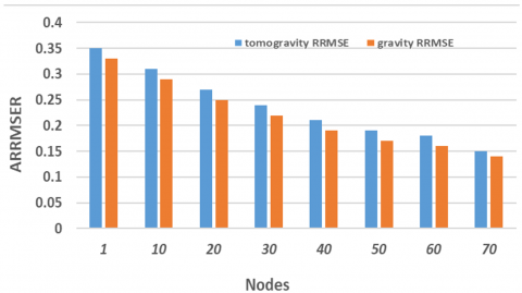
In this study, to estimate the initial size for flow the gravity model and the tomogravity model are used. These estimates serve as the basis for selecting flows size. Figure 2 illustrates the ARRMSER of the last flow environments resulting from these both models. The results clearly show that the tomogravity model significantly superior on the gravity model, with the performance gap reaching up to 35% in some scenarios. This highlights the tomogravity model's superior accuracy in flow size estimation, making it a more reliable choice for Flow Volume computation.
Figure 2. Different estimation results from two models in network 3
ALO2 was developed as an enhancement of ALO1 by replacing the integer programming approach with a probabilistic placement strategy for sd flows. To evaluate the two algorithms, we compared their accuracy and computational efficiency on T2 and T3. Both networks had fixed routing paths and pre-determined router locations. Table 1 presents the Average Relative Root Mean Square Error (ARRMSE) according to the varying size of TCAM for both ALO1 and ALO2 across T2 and T3. The results show that for most TCAM sizes, the ARRMSE values for both ALO remain relatively close, with differences not exceeding 6%. This indicates that ALO2, despite simplifying the flow placement process, achieves a comparable accuracy to ALO1. One notable observation is that for T2, ALO1 generally exhibits slightly higher ARRMSE values than ALO2, particularly for larger TCAM sizes (e.g., 58 and 66 entries). This suggests that ALO2 performs better in terms of maintaining lower relative errors in this topology. However, for T3, ALO1 and ALO2 demonstrate similar performance, with minor variations across different TCAM sizes. Additionally, for TCAM sizes of 55 and above, we observe a general stabilization of ARRMSE values, indicating that beyond a certain TCAM threshold, increasing the table size does not significantly impact accuracy. This suggests that network operators can achieve efficient flow management with moderate TCAM sizes, reducing hardware overhead while maintaining high accuracy.
Table 1. Comparison between algorithms 1 and 2 in two topologies
|
TCAM Size |
ALO1 ARRMSE (T3) |
ALO2 ARRMSE (T3) |
ALO1 ARRMSE (T2) |
ALO2 ARRMSE (T2) |
|
22 |
- |
- |
0.14 |
0.13 |
|
27 |
- |
- |
0.12 |
0.12 |
|
32 |
- |
- |
0.12 |
0.12 |
|
37 |
- |
- |
0.12 |
0.12 |
|
42 |
- |
- |
0.12 |
0.12 |
|
47 |
- |
- |
0.12 |
0.12 |
|
52 |
- |
- |
0.12 |
0.12 |
|
53 |
- |
- |
0.12 |
0.12 |
|
54 |
- |
- |
0.12 |
0.12 |
|
50 |
0.15 |
0.14 |
0.35 |
0.32 |
|
55 |
0.14 |
0.13 |
0.30 |
0.28 |
|
58 |
0.13 |
0.12 |
0.26 |
0.24 |
|
62 |
0.12 |
0.12 |
0.23 |
0.21 |
|
66 |
0.12 |
0.12 |
0.18 |
0.17 |
|
70 |
0.12 |
0.12 |
0.16 |
0.15 |
We analyzed the computation time for both ALO on two network topologies using an Intel Xeon processor with 16GB of memory. To ensure a realistic and practical evaluation in SDN, we initially fixed the TCAM size at 50 entries per node. This configuration aligns with common TCAM limits in medium-scale SDN deployments, where switches typically allocate between 32 and 128 TCAM entries for flow table management. Choosing 50 entries provides a balanced trade-off between hardware constraints and resource availability while serving as a reference baseline for subsequent scalability analysis. The results, summarized in Table 2, demonstrate a significant reduction in execution time when using ALO2 compared to ALO1. For T2, ALO1 takes approximately 0.2546 s, while ALO2 completes execution in just 0.0998 s, representing a 60.8% reduction in processing time. The efficiency gain is even more pronounced in T3, where ALO1 takes 59.4678 s, whereas ALO2 requires only 4.9581 s, yielding an impressive 91.7% improvement in execution speed. These results highlight the computational efficiency of ALO2, particularly for larger and more complex network topologies like T3. The significant reduction in execution time makes ALO2 more scalable and practical for real-world SDN deployments, where minimizing processing delays is critical for applications such as real-time traffic engineering and flow management.
Table 2. Execution time (fixed TCAM size, 50 entries per node)
|
|
T2 |
T3 |
|
ALO1 |
0.2546s |
59.4678s |
|
ALO2 |
0.0998s |
4.9581s |
To further evaluate scalability, we conducted additional experiments with varying TCAM sizes (20-100) entries per node). As shown in Table 3, ALO2 exhibits linear growth in execution time, completing in less than 10 seconds even for 100 TCAM entries. In contrast, ALO1 demonstrates quadratic growth, exceeding 120 seconds for large TCAM sizes. This difference in scalability makes ALO2 more suitable for real-time applications, where flow management updates must be completed within sub-30-second response times to ensure optimal network performance.
Table 3. Execution time (T2 and T3)
|
TCAM Size |
ALO1 (T2) |
ALO2(T2) |
ALO1(T3) |
ALO2 (T3) |
|
20 |
0.15s |
0.05s |
10.2s |
0.8s |
|
40 |
0.25s |
0.07s |
30.5s |
2.5s |
|
60 |
0.40s |
0.15s |
62.5s |
5.0s |
|
80 |
0.60s |
0.20s |
90.0s |
8.0s |
|
100 |
0.85s |
0.25s |
120.0s |
10.0s |
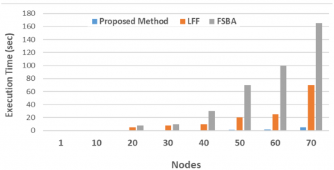
To further validate ALO2 efficiency, we compared its execution time with two other methods, LFF [13] and FSBA [16], in T3 using fixed the TCAM size at 50 entries per node. Figure 3 illustrates the computation time respect to numeral of devices or nodes. ALO2 consistently maintained a lower execution time, with its growth curve remaining much flatter compared to LFF and FSBA, proving its scalability and computational advantage in complex networks.
The efficiency (eff) of TCAM utilization is defined as:
eff $=\frac{\text { total number of useful sd flows }}{\text { total number of added sd flows }}$ (6)
Figure 3. Execution time of three methods with fixed TCAM Size, 50 entries per node
A useful sd flow contributes to increasing the rate of volume M. A higher eff value indicates more efficient utilization of the TCAM entries, leading to better estimation results. Table 4 presents a comparative analysis of TCAM utilization efficiency across different ALO in T1 and T2, with a fixed number of SDN nodes while varying the TCAM size. The results demonstrate that the proposed method consistently achieves 100% utilization, significantly outperforming conventional methods such as LFF and FSBA, whose efficiency declines as TCAM size increases. The proposed method’s superior performance can be attributed to the RAISPR mechanism, which effectively manages flow entries to optimize TCAM space. In contrast, conventional methods struggle with flow selection, leading to suboptimal utilization and inefficiencies. For example, in T1, LFF efficiency drops from 0.6 at size 22 to 0.5 at size 57, while FSBA declines from 0.7 to 0.6 over the same range. Similarly, in T2, FSBA efficiency falls from 0.8 at size 22 to 0.5 at size 62, illustrating its reduced ability to manage flow entries efficiently as TCAM capacity grows. This trend is expected, as conventional methods fail to dynamically adapt to increasing TCAM capacity, making it more difficult to select independent flow entries efficiently.
Table 4. Efficiency of three methods in two topologies
|
TCAM Size |
T1 Proposed |
T1 [13] |
T1 [16] |
T2 Proposed |
T2 [13] |
T2 [16] |
|
17 |
1 |
0.5 |
0.6 |
- |
- |
- |
|
22 |
1 |
0.6 |
0.7 |
1 |
0.9 |
0.8 |
|
27 |
1 |
0.7 |
0.75 |
1 |
0.85 |
0.75 |
|
32 |
1 |
0.7 |
0.8 |
1 |
0.8 |
0.7 |
|
37 |
1 |
0.65 |
0.75 |
1 |
0.75 |
0.65 |
|
42 |
1 |
0.6 |
0.7 |
1 |
0.7 |
0.6 |
|
47 |
1 |
0.55 |
0.65 |
1 |
0.65 |
0.55 |
|
52 |
1 |
0.5 |
0.6 |
1 |
0.6 |
0.5 |
|
57 |
1 |
0.5 |
0.6 |
1 |
0.55 |
0.5 |
|
62 |
- |
- |
- |
1 |
0.5 |
0.5 |
As a result, their effectiveness diminishes, particularly in large-scale SDN deployments where optimal TCAM utilization is critical for maintaining high network performance. The findings underscore the practical advantages of the proposed method, making it well-suited for real-world SDN environments where TCAM resources are often a limiting factor. By ensuring full utilization, the proposed method provides:
In contrast, the limitations of LFF [13] and FSBA [16] indicate that these conventional strategies may not be viable for large-scale SDN implementations. Their decreasing efficiency with larger TCAM sizes highlights their inability to manage flow entries dynamically, reinforcing the need for intelligent, adaptive methods like the one proposed in this study.
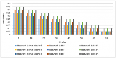
Our proposed approach demonstrates its ability to fully utilize the TCAM entries, ensuring optimal performance in traffic measurement scenarios. Lastly, the performance of the proposed framework was compared against two existing methods, LFF and FSBA, across three network topologies. In these networks, programable nodes constituted approximately 14% of the total nodes. The quantity of TCAM used was set to 29% of the overall quantity of devices in each T. Figure 4 and Table 5 illustrate the results of the comparison. The proposed framework consistently outperformed LFF and FSBA. For example, in T1, the maximum estimation error of FSBA was reduced from 11.23% to 2.69%, while LFF saw a reduction from 6.88% to 1.28%. Furthermore, as the TCAM size increased, the rate of performance improvement was significantly higher for the proposed framework compared to the other two methods, as shown in Table 5.
Figure 4. Assessment of three approaches in different network conditions
Table 5. Efficiency comparison (A: T1-Proposed, B: T1-LFF, C: T1-FSBA, D: T2-Proposed, D: T2-LFF, F: T2-FSBA, G: T3-Proposed, H: T3- LFF, I: T3-FSBA)
|
TCAM Size |
A |
B |
C |
D |
E |
F |
G |
H |
I |
|
16 |
0.3 |
0.3 |
0.3 |
- |
- |
- |
- |
- |
- |
|
19 |
0.2 |
0.3 |
0.3 |
- |
- |
- |
- |
- |
- |
|
22 |
0.1 |
0.2 |
0.3 |
0.4 |
0.4 |
0.4 |
- |
- |
- |
|
25 |
0.1 |
0.2 |
0.2 |
0.3 |
0.4 |
0.3 |
- |
- |
- |
|
28 |
0.2 |
0.1 |
0.2 |
0.2 |
0.3 |
0.3 |
- |
- |
- |
|
31 |
0.1 |
0.1 |
0.2 |
0.2 |
0.2 |
0.3 |
- |
- |
- |
|
34 |
0.1 |
0.15 |
0.1 |
0.2 |
0.2 |
0.2 |
- |
- |
- |
|
37 |
0.1 |
0.15 |
0.2 |
0.1 |
0.2 |
0.2 |
- |
- |
- |
|
40 |
0.2 |
0.15 |
0.1 |
0.1 |
0.1 |
0.2 |
- |
- |
- |
|
49 |
- |
- |
- |
- |
- |
- |
0.3 |
0.3 |
0.3 |
|
56 |
- |
- |
- |
- |
- |
- |
0.2 |
0.2 |
0.2 |
|
63 |
- |
- |
- |
- |
- |
- |
0.2 |
0.2 |
0.2 |
|
70 |
- |
- |
- |
- |
- |
- |
0.2 |
0.1 |
0.2 |
|
77 |
- |
- |
- |
- |
- |
- |
0.1 |
0.1 |
0.2 |
|
84 |
- |
- |
- |
- |
- |
- |
0.2 |
0.2 |
0.2 |
|
91 |
- |
- |
- |
- |
- |
- |
0.1 |
0.1 |
0.2 |
|
98 |
- |
- |
- |
- |
- |
- |
0.1 |
0.2 |
0.1 |
|
105 |
- |
- |
- |
- |
- |
- |
0.2 |
0.2 |
0.1 |
Another notable observation is that the performance of the proposed framework improved consistently with increasing TCAM size. This behavior contrasts with LFF and FSBA, where, performance gains were inconsistent. The inconsistency in LFF and FSBA can be attributed to their inability to ensure that every flow insert to the FT be a useful info about the Flow Volume. In contrast, the proposed method leverages the RAISPR, which guarantees that every flow added to the FT enhances the estimation accuracy, leading to steady performance improvement as the TCAM size grows.
From the above, the accuracy of Flow Volume estimation in the proposed framework depends on the initial weight estimation provided by the tomogravity model. While the tomogravity model has been shown to improve accuracy over the standard gravity model, its assumptions may not always hold under real-world network conditions. To assess the framework’s robustness against potential inaccuracies in initial weight estimation, we conduct a sensitivity analysis by introducing controlled perturbations to the estimated weights. To evaluate the impact of weight estimation errors, we introduce variations of ±10%, ±20%, and ±30% to the initial weight values generated by the tomogravity model. The perturbed weights are then used in the flow selection process, and the resulting Flow Volume estimation accuracy is measured using the ARRMSE. Table 6 presents the ARRMSE values under different levels of perturbation in initial weights for T2 and T3.
Table 6. Impact of initial weight perturbation on ARRMSE for T2 and T3
|
Perturbation Level |
ARRMSE (T2) |
ARRMSE (T3) |
|
No Perturbation |
0.12 |
0.14 |
|
±10% Variation |
0.13 |
0.15 |
|
±20% Variation |
0.15 |
0.18 |
|
±30% Variation |
0.18 |
0.22 |
From the results, we observe that moderate variations (±10% to ±20%) do not significantly degrade accuracy, with an ARRMSE increase of only 0.01 to 0.03. However, at higher perturbations (±30%), the estimation accuracy begins to degrade more noticeably, highlighting the sensitivity of the framework to large deviations in initial weight estimation. For future enhancements and to minimize the impact of inaccurate initial weights, the following strategies can be integrated into the framework:
This sensitivity analysis demonstrates that while the framework is relatively stable under moderate weight variations, incorporating adaptive mechanisms can further enhance its resilience in real-world deployments.
The scalability of the proposed framework is a crucial factor in ensuring its applicability in large-scale SDN deployments. While ALO2 significantly reduces computational complexity compared to ALO1, its effectiveness in large-scale networks and under dynamic traffic conditions warrants further analysis.
7.1 Scalability considerations
The computational complexity of ALO2, making it feasible for medium to large-scale networks. However, as network size increases, the number of possible sd flow combinations grows exponentially, which may introduce additional overhead in managing flow entries within the TCAM. To address this, the following optimizations can be considered:
7.2 Performance under dynamic traffic conditions
Dynamic traffic conditions pose challenges in maintaining accurate Flow Volume estimation. The proposed framework mitigates these issues through:
This paper introduced a novel framework to address the FVE problem in a programable framework using IP networks. A key advantage of this framework is its ability to ensure that every flow added to a programable node increases the rate of the primary structure for FVE. In simple terms, its assurances that no drift supplementary for size can be derivative from the data of additional flows previously or already in the FT of wholly programable nodes. This feature significantly enhances the efficiency of TCAM utilization within FT. Through performance evaluations, we demonstrated that this framework delivers substantial improvements over existing methods. Accurate FVE plays a crucial role in solving challenges like routing optimization and network provisioning. The advancements presented in this work have the potential to fundamentally influence the way routing and traffic management are approached in future programable networks. Although the current evaluation focuses on networks with up to 60 nodes, real-world SDN deployments often involve thousands of nodes. To validate the framework’s scalability, future work will extend the evaluation to larger topologies, leveraging datasets from real-world backbone networks. Additionally, experiments under dynamic traffic scenarios will be conducted to assess the robustness of the heuristic approach in handling sudden traffic spikes and congestion events.
The work is supported by eköp-24 University Excellence Scholarship Program of the Ministry for Culture and Innovation from the source of the National Research, Development, and Innovation Fund.
|
RV |
Routing volume |
|
eff |
Efficiency |
|
FVESDN |
Traffic volume estimation SDN |
|
FV |
Traffic volume |
|
LL |
Link loads |
|
nl |
Normalization |
|
RAM |
Rate of volume |
|
v |
Vector |
|
at |
Actual traffic |
|
wei |
Wight |
|
M |
Volume |
|
BV |
Binary volume |
|
NO |
Total number |
|
sd |
source-destination |
|
d |
Destination-based flow |
|
SN |
Sets of nodes |
|
TCAM |
Ternary content addressable memory |
|
Subscripts |
|
|
z |
Set of all source-destination |
|
sd |
Source-destination |
|
i |
Link |
|
sl |
Sets of links |
[1] Ali, T.E., Ali, F.I., Dakić, P., Zoltan, A.D. (2025). Trends, prospects, challenges, and security in the healthcare internet of things. Computing, 107(1): 28. https://doi.org/10.1007/s00607-024-01352-4
[2] Ali, T.E., Ali, F.I., Abdala, M.A., Morad, A.H., Gódor, G., Zoltán, A.D. (2024). Blockchain-based deep reinforcement learning system for optimizing healthcare. Infocommunications Journal, 16(3): 89-100. https://doi.org/10.36244/ICJ.2024.3.9
[3] Prasanth, L.L., Uma, E. (2024). A computationally intelligent framework for traffic engineering and congestion management in software-Defined network (SDN). EURASIP Journal on Wireless Communications and Networking, 2024(1): 63. https://doi.org/10.1186/s13638-024-02392-2
[4] Gilliard, E., Liu, J.S., Aliyu, A.A., Juan, D., Jing, H., Wang, M. (2024). Intelligent load balancing in data center software-defined networks. Transactions on Emerging Telecommunications Technologies, 35(4): e4967. https://doi.org/10.1002/ett.4967
[5] Ali, T.E., Morad, A.H., Abdala, M.A. (2020). Traffic management inside software-defined data centre networking. Bulletin of Electrical Engineering and Informatics, 9(5): 2045-2054. https://doi.org/10.11591/eei.v9i5.1928
[6] Tuncer, D., Charalambides, M., Clayman, S., Pavlou, G. (2015). Adaptive resource management and control in software defined networks. IEEE Transactions on Network and Service Management, 12(1): 18-33. https://doi.org/10.1109/TNSM.2015.2402752
[7] Du, Q., Cui, X., Tang, H.Y., Chen, X.X. (2024). Review of load balancing mechanisms in SDN-based data centers. Journal of Computer and Communications, 12(1): 49-66. https://doi.org/10.4236/jcc.2024.121004
[8] Iesar, H., Iqbal, W., Abbas, Y., Umair, M.Y., Wakeel, A., Illahi, F., Saleem, B., Muhammad, Z. (2024). Revolutionizing data center networks: Dynamic load balancing via floodlight in SDN environment. In 2024 5th International Conference on Advancements in Computational Sciences (ICACS), Lahore, Pakistan, pp. 1-8. https://doi.org/10.1109/ICACS60934.2024.10473246
[9] Maity, I., Giambene, G., Vu, T.X., Kesha, C., Chatzinotas, S. (2024). Traffic-Aware resource management in SDN/NFV-based satellite networks for remote and urban areas. IEEE Transactions on Vehicular Technology, 73(11): 17400-17415. https://doi.org/10.1109/TVT.2024.3420807
[10] Isyaku, B., Bakar, K.B.A., Nagmeldin, W., Abdelmaboud, A., Saeed, F., Ghaleb, F.A. (2023). Reliable failure restoration with Bayesian congestion aware for software defined networks. Computer Systems Science & Engineering, 46(3): 3729-3748. https://doi.org/10.32604/csse.2023.034509
[11] Liu, Z., Xie, S., Zhang, H., Zhou, D., Yang, Y. (2024). A parallel computing framework for large-scale microscopic traffic simulation based on spectral partitioning. Transportation Research Part E: Logistics and Transportation Review, 181: 103368. https://doi.org/10.1016/j.tre.2023.103368
[12] Yuan, X., Qiao, Y., Wei, Z., Zhang, Z., Li, M., Zhao, P., Hu, R., Li, W. (2025). Diffusion models meet network management: Improving traffic matrix analysis with diffusion-based approach. IEEE Transactions on Network and Service Management, 22(2): 1259-1275. https://doi.org/10.1109/TNSM.2025.3527442
[13] Wang, Y., Othman, M., Choo, W.O., Liu, R., Wang, X. (2024). DFRDRL: A dynamic fuzzy routing algorithm based on deep reinforcement learning with guaranteed latency and bandwidth for software-defined networks. Journal of Big Data, 11(1): 150. https://doi.org/10.1186/s40537-024-01029-x
[14] Esmaeilian, S., Dolati, M., Sadrhaghighi, S., Ghaderi, M. (2024). Coordinated sampling in SDNs with dynamic flow rates. In 2024 20th International Conference on Network and Service Management (CNSM), Prague, Czech Republic, pp. 1-7. https://doi.org/10.23919/CNSM62983.2024.10814381
[15] Hasan, M.K. (2024). Improving data aggregation performance in wireless sensor networks using software-defined networks. Journal of Intelligent Systems & Internet of Things, 12(2): 8-18. https://doi.org/10.54216/JISIoT.120201
[16] Xu, J., Pan, W., Tan, H., Cheng, L., Li, X. (2024). An adaptive congestion control optimization strategy in SDN-based data centers. Computers, Materials & Continua, 81(2): 2709-2726. https://doi.org/10.32604/cmc.2024.056925
[17] Blose, M., Akinyemi, L., Ojo, S., Faheem, M., Imoize, A.L., Khan, A.A. (2024). Scalable hybrid switching-driven software defined networking issue: From the perspective of reinforcement learning. IEEE Access, 12: 63334-63350. https://doi.org/10.1109/ACCESS.2024.3387273
[18] Lyu, G., Zheng, H. (2024). Spatial-temporal graph attention networks for dynamic traffic prediction of SDN. In 4th International Conference on Internet of Things and Smart City (IoTSC 2024), pp. 202-209. https://doi.org/10.1117/12.3035035
[19] Chen, B., Shi, X., Feng, T., Jiang, S., Zhai, Y., Ren, M., Liu, D., Wang, C., Gao, J. (2024). Construction and application of a private 5G standalone medical network in a smart health environment: Exploratory practice from China. Journal of Medical Internet Research, 26: e52404. https://doi.org/10.2196/52404
[20] Tiwari, A., Kumar, D. (2024). Sentinel shield: Leveraging ConvLSTM and elephant herd optimization for advanced network intrusion detection. EAI Endorsed Transactions on Scalable Information Systems, 11(6).
[21] Gangidi, A., Miao, R., Zheng, S., Bondu, S.J., Goes, G., Morsy, H., Puri, R., Riftadi, M., Shetty, A.J., Yang, J., Zhang, S., Fernandez, M.J., Gandham, S., Zeng, H. (2024). RDMA over ethernet for distributed training at meta scale. In Proceedings of the ACM SIGCOMM 2024 Conference, pp. 57-70. https://doi.org/10.1145/3651890.3672233
[22] Loehr, N.A. (2024). Advanced Linear Algebra. CRC Press. https://doi.org/10.1201/9781003484561
[23] Jurkiewicz, P. (2024). TopoHub: Synthetic global-scale backbone networks topologies. SoftwareX, 28: 101867. https://doi.org/10.1016/j.softx.2024.101867
[24] Xie, R.T. (2024). Traffic datsets: Abilene, GEANT, TaxiBJ. IEEE Dataport. https://doi.org/10.21227/7x3c-5p06
[25] GEANT/Abilene network topology data and traffic traces. University of Surrey, 2020. https://doi.org/10.15126/surreydata.00807659