Juan Sebastian Bonilla-Uribe*![]() | Luis M. Moran Yañez
| Luis M. Moran Yañez![]() | Yvan Huaricallo
| Yvan Huaricallo![]() | Jorge L. Capuñay-Sosa
| Jorge L. Capuñay-Sosa![]() | Nahum O. Cubas Parimango
| Nahum O. Cubas Parimango![]() | Johnny H. Ccatamayo Barrios
| Johnny H. Ccatamayo Barrios![]() | Leyla F. Guerrero Mendoza
| Leyla F. Guerrero Mendoza![]()
© 2025 The authors. This article is published by IIETA and is licensed under the CC BY 4.0 license (http://creativecommons.org/licenses/by/4.0/).
OPEN ACCESS
This study aims to develop a predictive model based on Python to assess the mechanical behavior of "reactive" soils through static triaxial tests, considering key geomechanical factors. The tests were conducted on soil samples taken from depths of 1.5 to 2.0 meters (shallow) and from 16.5 to 18.0 meters (deep). The data obtained, which include pore pressure records, displacements, and deformation, were processed and analyzed using Python libraries such as NumPy and Pandas. The model is based on linear regressions and statistical techniques to analyze the relationships between variables such as soil density, cohesion, and the friction angle. The results showed that the model was able to simulate the soil behavior under different static loading conditions with high accuracy, considering confinement pressure and soil density. The analysis indicated that pore pressure has a significant impact on the shear strength of deep clays, with a 25% decrease in strength under saturated conditions. The integration of Python allowed for the automation of complex calculations and optimization of the analysis, providing an effective tool for conducting rapid and precise assessments in geotechnical projects. This study focuses exclusively on static conditions, leaving seismic conditions for future research.
soil mechanical analysis, static triaxial tests, Python, predictive model, physical factors, geotechnical applications, experimental methodology
Soil behavior is a critical aspect in civil and geotechnical engineering [1], as it determines the stability and safety of structures built on or within it [2, 3]. The physical and mechanical properties of the soil directly influence the performance of buildings, bridges, roads, and other infrastructures [4]. Understanding how soils respond to different loading conditions is crucial for anticipating failures and mitigating risks associated with landslides, settlements, or other geotechnical phenomena [5]. The diversity of soils in different regions of the world represents a significant challenge for geotechnical engineers [6]. These vary from highly cohesive clays to loose sands, each with unique characteristics that affect their behavior under stress [7-9]. The stability of a structure depends on properties such as density, cohesion, friction angle, and bearing capacity [9, 10], which not only differ between locations but also change over time due to factors such as moisture, temperature, or earthquakes [10]. Therefore, analyzing the soil in detail for each project is vital to design structures capable of resisting local conditions, ensuring their integrity, and avoiding stability issues [11, 12].
Soil mechanics, as a key subdiscipline of geotechnical engineering, focuses on studying the physical properties and mechanical behavior of the soil, critical aspects for structural safety [13, 14]. Among laboratory tests, the triaxial test stands out for its ability to replicate real stress conditions. This method, especially in its static version, allows for the accurate assessment of shear strength, deformation, and failure mechanisms of the soil under controlled stress paths. Its robustness makes it an indispensable tool for obtaining data that guides geotechnical design, simulating realistic scenarios, and measuring essential parameters with high reliability, positioning it as a cornerstone in the research and practice of this discipline.
Given the importance of triaxial data, geotechnics has moved toward predictive models that integrate this information to forecast soil behavior under various conditions. These models are essential as they simulate responses to loads and environmental factors, optimizing safe and efficient designs. By combining experimental data with advanced techniques, they enable the evaluation of multiple scenarios without additional tests, saving time and resources. Moreover, their ability to address soil variability and complex phenomena improves accuracy, being key to mitigating risks in extreme events such as earthquakes or floods, and ensuring the durability of structures [15].
In this context, the integration of Python into soil mechanics marks a significant advancement for geotechnical analysis and modeling. With libraries like NumPy, Pandas, and Matplotlib, Python efficiently processes large volumes of data, automates complex calculations, and presents results clearly. It also drives predictive models that simulate soil behavior under different loads [16, 17], transforming geotechnical studies by providing greater precision and reliability in infrastructure design. Its flexibility and accessibility make it ideal for engineers seeking advanced tools for their projects.
This research develops and validates a Python-based predictive model to assess soil behavior under physical conditions, using data from static triaxial tests. The goal is to increase the accuracy and reliability of mechanical property characterization, providing an advanced tool for safe and efficient designs. Furthermore, it aims to overcome limitations of traditional approaches by considering the inherent variability of the soil, with the potential to impact geotechnical practice in seismically active areas or complex soils.
For this study, a comprehensive review of prior works on soil mechanics and geotechnics was conducted. Notably, a study [18] investigated the strength and dilatancy of sand stabilized with colloidal-silica gel, revealing enhanced shear strength and reduced dilation post-stabilization. The findings underscore the importance of nonlinear stress-dilatancy relationships in modeling soil behavior. Similarly, another study [19] examined tunneling-induced ground movements, highlighting the abrupt volume loss in collapsible soils under load, which is critical for excavation stability. These studies emphasize the challenges of reactive soils, such as expansive and collapsible types, whose mechanical responses to environmental factors like moisture, pressure, and load are complex [20]. Expansive soils exhibit swelling or contraction due to moisture fluctuations, leading to differential settlements or foundation failures, particularly in stabilized sands [20]. The heterogeneity and nonlinear properties of these soils, such as variable cohesion and friction angles, complicate traditional analyses. Collapsible soils, which experience sudden volume reduction under load, pose significant risks in tunneling projects.
Static triaxial tests are crucial for characterizing reactive soils, providing data on shear strength, dilation, and plastic deformation under controlled conditions. These tests also enable precise measurement of soil stiffness, particularly in unsaturated silty clays, which is essential for safe geotechnical designs. For instance, studies on soil-structure interactions in sandy soils highlight the importance of triaxial data for modeling tunneling effects [21]. However, manual analysis of triaxial data is time-consuming and error-prone, especially for highly variable reactive soils like saturated or unsaturated clays. This challenge is amplified in seismic zones, where numerical analyses of soil reinforcement are critical [22].
To address these limitations, predictive models for soft soils, incorporating simple parameters like cohesion and friction angle, have been developed to enhance design accuracy [23]. Python-based automation, utilizing libraries such as NumPy, Pandas, and Matplotlib, further streamlines triaxial data analysis [24]. Automated stress path adjustments improve the measurement of soil stiffness, supporting robust geotechnical designs. Python scripts can also precisely determine geotechnical properties and visualize results interactively, as demonstrated in studies on Nasiriyah soil [25]. This approach enhances efficiency and accuracy, revolutionizing the design of structures on complex soils. Building on these advancements, the proposed model employs Python to analyze static triaxial data for reactive soils, incorporating nonlinear properties like dilation and failure modes in clays and unsaturated soils. It draws on methodologies from prior studies to automate calculations and enable dynamic adjustments for projects in geotechnically challenging or seismic areas [25].
This paper presents the development and validation of a predictive model for reactive soils, detailing Python-based data processing and algorithms for optimizing stress paths. The model is validated against experimental data and compared with established frameworks, demonstrating enhanced accuracy and efficiency. The study explores implications for geotechnical engineering and proposes future applications in nonlinear soil-structure interactions [25].
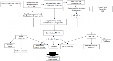
The methodology of this study was organized into a series of key stages, carefully designed to ensure maximum accuracy and reliability in the obtained results. The research process began with conducting static triaxial tests in a controlled laboratory environment, which allowed for the collection of critical data on soil behavior under various loading conditions. Subsequently, a thorough and rigorous analysis of this data was carried out using Python, a powerful tool that facilitated the development of a highly robust predictive model, as shown in Figure 1.
Figure 1. Model process
The model presented in Figure 1 not only integrates the experimental results but also allows for the simulation of complex scenarios, providing a more comprehensive and accurate assessment of soil behavior in different geotechnical contexts.
2.1 Soil sample preparation
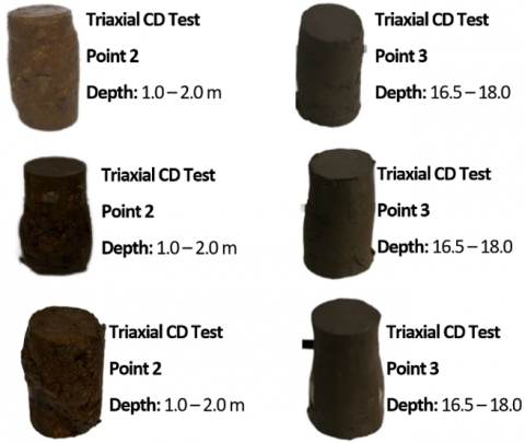
The first stage of this study involved the collection and preparation of soil samples, which were obtained from different depths of the ground to ensure adequate representativeness of the geotechnical layers of the subsurface. Samples were extracted from two types of strata: shallow samples, taken at depths ranging from 1.0 to 2.0 meters, and deep samples, obtained from depths between 16.50 and 18.0 meters. To ensure the geotechnical representativeness of the soils, samples from distinct regions were included, with details described below:
Surface Sample: Silty sand with high plasticity, dark orange-brown in color, extracted from a shallow depth of 1.0 to 2.0 meters, also obtained through rotary drilling to ensure the collection of undisturbed samples.
Deep Sample: Clay with the presence of light brown sand, extracted from a depth of 16.50 to 18.0 meters, using the rotary drilling method to preserve sample integrity.
To ensure the quality of the experimental results, the samples were subjected to homogenization and conditioning processes to guarantee uniformity in terms of moisture content and density, as seen in Figure 2.
These procedures were carried out in accordance with the guidelines established by ASTM D1587-00 for undisturbed sample extraction and ASTM D698-00 for compaction tests.
This rigorous preparation process is crucial, as any variability in the initial properties of the samples could significantly influence the results of the tests, affecting the interpretation of the geotechnical data. During this preparation phase, three samples were evaluated for each depth section, with a total of 17,200 data points recorded for the full test, allowing for a precise and representative assessment of the soil behavior under the specific ground conditions.
Figure 2. Standardized sample preparation
2.2 Static triaxial tests
Static triaxial tests, conducted under carefully controlled conditions, are essential for determining the mechanical properties of the soil, such as its shear strength, behavior under various confinement pressures, and deformation capacity. To conduct these tests, a triaxial cell equipped with high-precision sensors was used, capable of measuring axial and radial stresses, as well as pore pressures. The tests followed the procedures outlined in the ASTM D4767-11 standard, which specifies the methods for performing consolidated and drained triaxial tests on cohesive soils. Figure 3 shows the samples after they had been saturated, consolidated, and failed during the triaxial test.
Figure 3. Post-failure specimens after triaxial testing
The samples were subjected to variable confinement pressures, simulating the actual loading conditions found in the field, and controlled drainage conditions were implemented to ensure that the shear strength parameters were measured with the highest accuracy. The rigorous control of experimental conditions allowed for reliable results that reflect the soil's behavior under different loading scenarios, which is essential for the proper design of geotechnical structures such as foundations, slopes, and retaining walls. Furthermore, these tests provided valuable data to feed the predictive model developed in the later stages of the study.
2.3 Python-based data analysis
Once the data obtained from the triaxial tests were collected, they were analyzed using Python, a programming language widely used in engineering due to its flexibility, ability to handle large volumes of data, and its extensive library of specialized tools.
First, the NumPy and Pandas libraries were used for data manipulation and processing, allowing for statistical calculations as well as the efficient transformation and organization of data sets. It is worth noting that, since triaxial tests include multiple stages (saturation, consolidation, and failure), several .log files are generated and organized for each of these stages. The number of .log files may vary depending on the sample's moisture content; for example, if the sample has high moisture, the saturation process may require fewer .log files compared to low-moisture samples, as seen in the different strata of the samples.
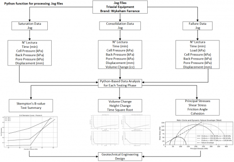
The data cleaning and normalization process was crucial at this stage, as it allowed for the elimination of any potential anomalies or errors in the data that could distort the analysis results. Through the use of advanced exploratory data analysis techniques, outliers were identified and corrected, ensuring the conditions for obtaining representative data of the soil's properties. This phase is essential to ensure that the results are as close as possible to the actual ground conditions, as illustrated in the flowchart of the saturation data cleaning process in triaxial tests (Figure 4).
Figure 4. Workflow for automated saturation data cleaning in triaxial testing
Figure 5. Consolidation data processing workflow for triaxial testing
Figure 6. Failure data processing workflow for triaxial testing
The saturation analysis was carried out with the automation of complex calculations, allowing for the determination of critical geotechnical parameters. These data were processed and filtered according to the quality and quantity of the .log files generated during the saturation stage. As shown in Figure 4, this process ensures that only representative data are considered for the analysis of soil strength.
Once these calculations were performed, the procedures for consolidation and failure were also automated, facilitating the analysis of shear strength and deformability under different loading conditions. In the consolidation phase, confinement and back pressure were adjusted according to the results obtained during saturation, and data on volume change and displacement were recorded, as shown Figure 5.
During the failure phase, deformation and load data were recorded under a constant deformation rate, with particular attention to the values of chamber pressure and back pressure. As shown in Figure 6 the failure data were processed, and any anomalies in the results were corrected before the final interpretation.
The automation of the analysis allowed for greater accuracy and speed in calculating geotechnical parameters such as shear strength, resulting in a more efficient and reliable interpretation of the data obtained during the different phases of the triaxial test.
2.4 Design, simulation, and experimental validation of a predictive model
The predictive model developed in this study is based on advanced machine learning and regression techniques, which allowed for the identification of patterns and complex relationships between key variables studied, such as soil density, cohesion, and friction angle. Multiple regression algorithms were used to analyze the nonlinear relationships between these variables, providing a deeper understanding of the soil's mechanical behavior.
This study focuses on evaluating the influence of geomechanical factors, such as confinement pressure and soil density, on the mechanical behavior of the soil, excluding seismic conditions due to the static nature of the triaxial tests. Models based on exploratory data analysis and regression algorithms were used to obtain the predictions, without employing complex cross-validation techniques like K-fold, which are considered more suitable for other types of models, such as those used in more advanced supervised learning.
To ensure the reliability of the predictive model, internal validation methods were used, such as comparing the results obtained with additional experimental data that were not used in the training phase. This process allowed for validating the model's ability to generalize to new conditions, confirming that the generated predictions are consistent with the experimental data and actual geotechnical conditions.
While the K-fold cross-validation method was not implemented in this study, it is an approach that could be considered in future research related to more complex predictive models, particularly in scenarios where further optimization of the model's accuracy is sought by validating different data subsets.
In the simulation phase, tests were carried out under different loading scenarios, using parameters obtained from the triaxial tests. These simulations included variations in confinement pressure and soil density, replicating real geotechnical conditions to evaluate the soil's behavior under different static loading conditions. The results of the simulations were validated by comparing the model's predictions with additional experimental data not used in the training phase. This comparison allowed for evaluating the model's ability to generalize and its applicability in real situations, showing a high correlation between the predictions and experimental data.
Model validation was crucial to confirm its accuracy and robustness. The success of the model during validation ensures its applicability in geotechnical projects, providing engineers with a valuable tool for planning and designing infrastructure, especially in areas with complex soils and variable loading conditions. This predictive model not only optimizes decision-making in geotechnical engineering but also offers greater reliability in risk assessment and the design of infrastructure resilient to seismic events.
This study laid the foundation for optimizing predictive models in the field of geotechnical engineering, and its implementation will be a key step in future research, where the use of techniques like K-fold cross-validation could be explored for a more rigorous evaluation of the model. Below, the scripts that support this study are presented.
Figure 7. Python implementation in the model to analyze the mechanical behavior of reactive soils
Saturation Analysis
Appendix A: The Python script used to calculate Skempton's B during the saturation phase is available in the final appendix of the article. This script processes the .rar files, extracts the relevant data, and calculates the Skempton’s B parameter. Details on its functionality can be found in the appendix.
Consolidation Analysis
Appendix B: The Python script used to calculate consolidation is available in the final appendix of the article. This script processes the data from the .log files and calculates additional columns such as the square root of time, height change, and other parameters related to soil consolidation. Details on its functionality can be found in the appendix.
Failure Analysis
Appendix C: The Python script used to calculate stresses and other parameters during the failure stage is available in the final appendix of the article. This script processes the data from the .log files and calculates parameters such as deviatoric stress, unit strains, and principal stresses, which are crucial for analyzing the soil's behavior during the failure phase. Details on its functionality can be found in Appendix C.
Elasticity Modulus Analysis
Appendix D: The Python script used to calculate the elasticity modulus is available in the final appendix of the article. This script processes the data from the .log files, calculates the elasticity modulus in the elastic region of the σ₁ vs. Unit Strain curve, and visualizes the interactive graph. Details on its functionality can be found in Appendix D.
Creep and Elasticity Analysis (MOHR MODEL)
Appendix E: The Python script used to generate the Mohr-Coulomb yield surface is available in the final appendix of the article. This script visualizes the yield surface based on the Mohr-Coulomb model, using the internal friction angle, cohesion, and stress range to show how the yield surface varies under different conditions. Details on its functionality can be found in Appendix E.
The following figure presents a diagram developed in Python to evaluate the mechanical behavior of "reactive" soils. This diagram is fundamental as it illustrates the predictive model that integrates various geotechnical and physical parameters for simulating soil behavior under static conditions.
Figure 7 provides a clear visual representation of how experimental data from the triaxial tests are organized and processed using Python, showing the interactions between key geotechnical variables such as cohesion, density, and other relevant parameters. Additionally, it should be emphasized that this diagram not only validates the methodology used but also illustrates the potential of computational tools, such as Python, to model complex scenarios that are common in geotechnical engineering, enhancing the accuracy and reliability of the analysis.
3.1 Analysis of results
The analysis of the results obtained from the static triaxial tests and the predictive model developed with Python provides a detailed insight into the mechanical behavior of the soil under various conditions. Two types of soil samples, shallow and deep, were evaluated to study their behavior under different loading conditions. The samples were collected from specific depths, and the key findings are presented below, organized according to the main conditions of shallow and deep soil.
3.2 Saturation test results
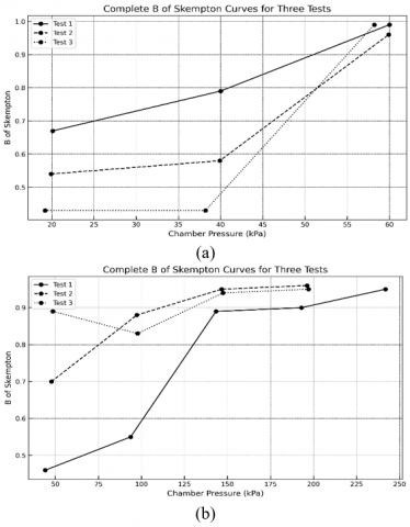
The saturation test evaluates the soil's ability to reach a fully saturated state under controlled conditions, which is crucial for understanding soil behavior in geotechnical applications, as shown in Figure 8. The variables analyzed include Skempton's B coefficient, chamber and pore pressures, and displacements, as shown in Table 1.
According to the results presented in Table 1, two types of soil samples were analyzed:
Analysis of Results:
Skempton's B Coefficient: The values close to 1 in both samples suggest that saturation was effective. The slight decrease in the deep sample (0.95) may be associated with its higher cohesion.
Displacements: In the shallow sample, the initial negative displacements indicate a slight contraction, while the displacements in the deep sample are higher, reflecting a plastic behavior typical of clayey soils.
Figure 8. Full saturation achieved in both surface and deep soil samples
Table 1. Experimental results of soil saturation tests
|
|
|
Cell Pressure (kPa) |
Pore Pressure (kPa) |
B Skempton |
Initial Displacement (mm) |
Final Displacement (mm) |
|
|
|
|
P1 |
40.00 |
63.5 |
0.99 |
7.767 |
-0.531 |
|
SURFACE |
Sample 1 1.50-2.00m |
P2 |
39.90 |
61.8 |
0.97 |
3.345 |
2.276 |
|
|
|
P3 |
38.20 |
60.8 |
0.99 |
3.933 |
2.515 |
|
|
|
P1 |
241.80 |
230.80 |
0.95 |
6.425 |
8.2 |
|
DEEP |
Sample 2 16.50-18.00m |
P2 |
196.30 |
185.70 |
0.95 |
9.325 |
11.467 |
|
|
|
P3 |
197.10 |
189.40 |
0.95 |
8.465 |
9.387 |
Table 2. Experimental results of the consolidation process
|
Height Change (mm) |
Pore Pressure (kPa) |
Cell Pressure (kPa) |
Back Pressure (kPa) |
σ₃ (kPa) |
|||
|
SURFACE |
Sample 1 1.50 - 2.00m |
P1 |
7.25 |
-22.1 |
80 |
50 |
30 |
|
P2 |
2.19 |
-55.9 |
100 |
39.9 |
60.1 |
||
|
P3 |
2.08 |
-111.4 |
180 |
60 |
120 |
||
|
DEEP |
Sample 2 16.50-18.00m |
P1 |
5.54 |
-47.6 |
300 |
200 |
100 |
|
P2 |
8.24 |
-97.7 |
399.9 |
200 |
199.9 |
||
|
P3 |
10.05 |
-113.5 |
430 |
30 |
400 |
||
3.3 Consolidation test results
Consolidation is a key process for assessing soil stability under sustained loads. The results obtained in Table 2 allow for the comparison of the mechanical behavior of shallow and deep soils in terms of height changes, pore pressure, and confinement under different loading conditions.
Analysis of Results:
Shallow Sample (1.50-2.00 m): At low confinement pressures, a high initial deformation is observed. As the confinement pressure increases, the deformation decreases significantly, reflecting soil stabilization.
Deep Sample (16.50-18.00 m): A more plastic behavior and slower consolidation are observed, which is typical of clayey soils. The consolidation process is more prolonged due to the low permeability of the clay.
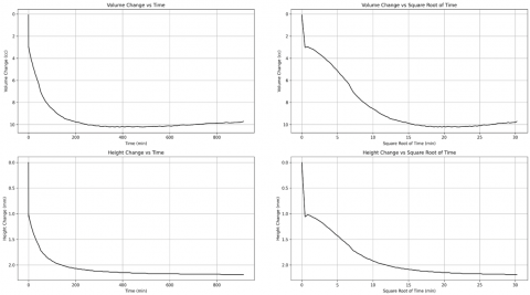
The curves in Figure 9 indicate a typical consolidation behavior, where most of the compression occurs in the early moments after the load is applied. The soil shows a rapid reduction in both volume and height initially, which is characteristic of low cohesion soils (such as silty sands, SM) when subjected to consolidation. As time progresses, the stabilization observed in the graphs indicates that primary consolidation is nearing completion, and any further change would be part of secondary consolidation, which is much slower.
Figure 9. Graphical interpretation of the consolidation stage for surface sample No. 1
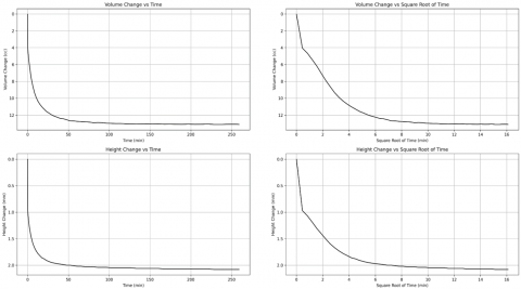
Figure 10. Graphical interpretation of the consolidation stage for surface sample No. 2
In this shallow SM soil sample from Figure 10, consolidation is rapid in the first few minutes, with significant compression and expulsion of water initially. The subsequent stabilization, characteristic of soils with high permeability and low cohesion, indicates that primary consolidation predominates, while secondary consolidation has a minimal impact.
This Figure 11 confirms the typical behavior of an SM soil under consolidation, where rapid deformation and water expulsion initially stabilize quickly. Primary consolidation dominates, with a secondary phase having minimal impact.
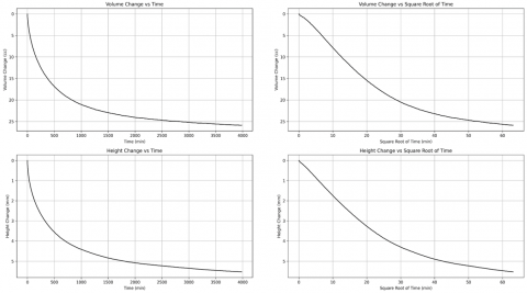
In this Figure 12 with a CL sample, consolidation is more prolonged due to the low permeability and higher cohesion, which causes a slower consolidation process. The curves reflect an extended primary consolidation, followed by gradual stabilization, typical of clayey soils.
Figure 11. Graphical interpretation of the consolidation stage for surface sample No. 3
Figure 12. Graphical interpretation of the consolidation phase for deep sample No. 1
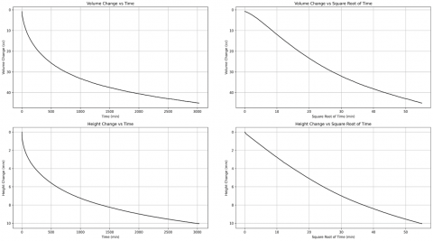
Figure 13. Graphical interpretation of the consolidation phase for deep sample No. 2
Figure 14. Graphical interpretation of the consolidation phase for deep sample No. 3
Figure 13 shows prolonged consolidation in CL soils, with a slow and continuous reduction in volume and height. Although primary consolidation continues to dominate, its duration is considerably longer than in less cohesive soils such as SM.
Figure 14 confirms prolonged consolidation in CL soils, with a controlled reduction in volume and height due to the soil's cohesion and low permeability. The curves reflect an extended primary consolidation process, with slow stabilization, typical of clayey soils.
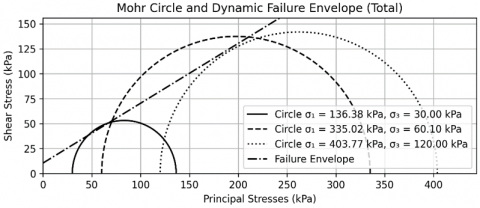
The failure envelope evaluates the soil behavior under increasing stresses until failure, using criteria such as Mohr-Coulomb to describe its resistance.
Analysis of Results from Table 3:
Shallow Sample (1.50-2.00 m): The progressive increases in confinement pressure (σ₃) and major principal stress (σ₁) show a typical response of granular soil under increasing stresses. The differences between total and effective stresses are small, indicating that pore pressure has a minor impact on the soil's strength.
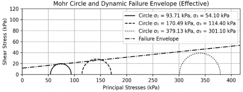
Deep Sample (16.50-18.00 m): The differences between total and effective stresses are more noticeable, reflecting the significant influence of pore pressure. In clayey soils like this sample, excess pore pressure reduces strength, making the maximum effective shear stress significantly lower than the total.
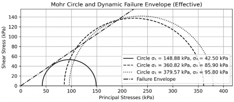
Analysis of Results from Table 4:
Shallow Sample (1.50-2.00 m): The strength is dominated by internal friction, with low total cohesion. The friction angle reflects the frictional behavior of the soil.
Deep Sample (16.50-18.00 m): The effective cohesion is higher in deep soils, suggesting that shear strength is more influenced by cohesion and pore pressure than in shallow soils.
Table 3. Shear failure test results
|
|
|
|
$\sigma_D$ (kPa) |
$\sigma_1$ (kPa) |
$\sigma_3$ (kPa) |
$\sigma_1^{\prime}$ (kPa) |
$\sigma_3^{\prime}$ (kPa) |
$\tau_{\max }$ (kPa) |
$\tau_{\text {max }}^{\prime}$ (kPa) |
$\left(\sigma_1+\sigma_3\right) / 2$ (kPa) |
$\left(\sigma_1^{\prime}+\sigma_3^{\prime}\right) / 2$ (kPa) |
|
|
|
P1 |
106.38 |
136.38 |
30.00 |
148.88 |
42.50 |
53.19 |
53.19 |
83.19 |
95.69 |
|
SURFACE |
Sample 1 1.50-2.00 m |
P2 |
274.92 |
335.02 |
60.10 |
360.82 |
85.90 |
137.46 |
137.46 |
197.56 |
223.36 |
|
|
|
P3 |
283.77 |
403.77 |
120.00 |
379.57 |
95.80 |
141.88 |
141.88 |
261.88 |
237.68 |
|
|
|
P1 |
39.61 |
139.61 |
100.00 |
93.71 |
54.10 |
19.81 |
19.80 |
119.80 |
73.90 |
|
DEEP |
Sample 2 16.50-18.00 m |
P2 |
56.09 |
255.99 |
199.90 |
170.49 |
114.40 |
28.04 |
28.04 |
227.94 |
142.44 |
|
|
|
P3 |
78.03 |
478.03 |
400.00 |
379.13 |
301.10 |
39.01 |
39.04 |
439.02 |
340.12 |
Table 4. Final parameters from the triaxial test
|
Mohr-Coulomb Parameters |
||||
|
Depth |
Sample |
Condition |
Friction Angle (°) |
Cohesion (kPa) |
|
SURFACE |
Sample 1 1.50-2.00 m |
Total |
30.96 |
10.2 |
|
Effective |
34.99 |
0 |
||
|
DEEP |
Sample 2 16.50-18.00 m |
Total |
5.71 |
6.8 |
|
Effective |
5.71 |
13.9 |
||
Figure 15. Mohr´s circle and dynamic failure envelope (total)-superficial
Figure 16. Mohr´s circle and dynamic failure envelope (effective)-superficial
Figure 17. Mohr´s circle and dynamic failure envelope (total)-profound
Figure 18. Mohr´s circle and dynamic failure envelope (effective)-profound
Figure 19. Stress path-Cambridge model- superficial
In granular soils, such as SM, total cohesion is low, which is related to their high permeability. Although total cohesion may appear due to factors such as compaction, its value remains relatively small. Figure 15 shows the soil's response under total stresses, without accounting for the effects of pore pressure.
In this Figure 16, the effects of pore pressure are removed, showing the effective stresses. The effective cohesion is reduced to zero, and the effective friction angle is higher, reflecting the true bearing capacity of the soil, dominated by friction.
For clayey soils such as CL, total cohesion is low due to pore pressure. Figure 17 shows the total stresses, which include pore pressure, reducing the overall strength of the soil.
The analysis of effective stresses reveals that the effective cohesion is considerably higher than the total cohesion, which reflects in Figure 18 the stabilizing effect of the soil structure under conditions of high saturation.
As observed in Figure 19, the behavior of the soil under conditions of total and effective stresses reflects a characteristic behavior of granular soils, where friction is the primary factor influencing shear strength.
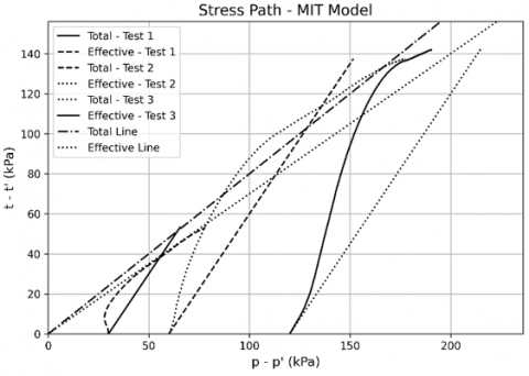
Figure 20 illustrates the behavior of both total and effective stresses using the MIT model. Both models exhibit linear and similar trajectories, which reinforces the importance of friction in shear strength.
Based on the interpretation of the graphs, the results of the two stress trajectories in the two soil types for the surface stratum can be concluded, as presented in Table 5.
Figure 20. Stress path + MIT model
Table 5. Stress-path analysis results (surface sample)
|
MIT |
||||
|
|
α |
a (kPa) |
||
|
SURFACE SM |
Muestra 1 1.50-2.00m |
Total |
38.66 |
0 |
|
Effective |
34.99 |
0 |
||
|
CAMBRIDGE |
||||
|
|
M |
Intercept (kPa) |
||
|
SURFACE SM |
Muestra 1 1.50-2.00m |
Total |
1.3 |
0 |
|
Effective |
1.2 |
0 |
||
Cohesion: In both models (Cambridge and MIT), cohesion is zero (0kPa), which is characteristic of granular soils such as SM.
Friction Angle: It reflects a purely frictional behavior, typical of granular soils. The values of M and α are suitable for sandy-silty soils, where strength depends entirely on interparticle friction.
Cambridge Model vs. MIT Model: Both models exhibit linear behavior with a slope governed by friction, showing no significant cohesion effects.
In Figure 21, the stress path under the MIT model is shown, which helps to visualize the shape of the stress trajectory under conditions of high confining pressure.
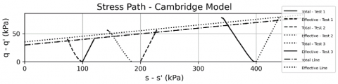
Similarly, Figure 22 illustrates the stress trajectory under the Cambridge model, highlighting the importance of cohesion in soils with low friction.
Figure 21. Stress path-MIT model
Figure 22. Stress path-Cambridge model
Table 6. Stress-path analysis results (deep sample)
|
MIT |
||||
|
|
α |
a (kPa) |
||
|
DEEP CL |
Sample 2 16.50-18.00 m |
Total |
5.71 |
9.2 |
|
Effective |
5.71 |
15.5 |
||
|
CAMBRIDGE |
||||
|
|
M |
Y-intercept (kPa) |
||
|
DEEP CL |
Sample 2 16.50-18.00 m |
Total |
0.1 |
29.6 |
|
Effective |
0.1 |
35.2 |
||
Based on the interpretation of the graphs, the results of the two stress trajectories in the two soil types for the deep stratum can be concluded, as presented in Table 6.
Significant Cohesion: In both the MIT and Cambridge models, the effective cohesion is considerable (15.5 kPa and 35.2 kPa, respectively), which is common in saturated clayey soils. This cohesion is the primary factor controlling the soil’s shear strength.
Low Friction Angle: The angle α and the parameter M are low, indicating minimal interparticle friction. In soils with high moisture content (115%), effective friction decreases significantly, leaving cohesion as the dominant factor.
Linear Trajectories: Both graphs display smooth or nearly horizontal trajectories, suggesting that the soil exhibits cohesive behavior with little additional resistance derived from friction.
Elastic Analysis
Based on the results obtained at the failure stage of the triaxial test, a linear behavior in the elastic modulus is observed for both evaluated soil types: the surface silty sand and the low-plasticity clay at depth, under varying confinement levels. This linear behavior allows for a preliminary assessment of each soil’s stiffness response under applied loading conditions, which is relevant for future geotechnical applications.
However, it is important to note that both soils exhibit specific limitations that must be considered for their use in geotechnical engineering:
Surface Silty Sand (Collapsible):
The silty sand exhibits high variability in its elastic modulus, with a significant increase in values as confining pressure rises. This indicates that the soil has an adequate hardening capacity under confined loading but also reveals its high sensitivity to factors such as density and moisture. This variability could lead to differential settlements if not properly controlled during construction.
For shallow geotechnical applications, the silty sand may be suitable provided that efficient compaction methods and strict quality controls are implemented. This approach can minimize variability in its behavior and ensure consistent, predictable performance throughout the structure’s service life.
Low-Plasticity Clay at Depth (Expansive):
In contrast, the deep soil, characterized by low-plasticity clay, exhibits a significantly lower elastic modulus, implying limited stiffness even under high confinement levels. This property is typical of clays and suggests that the soil is prone to long-term plastic deformations, particularly in deep foundation projects or structures subjected to permanent loads.
Due to its compressible behavior, the use of this clay in structural applications requires mitigation measures, such as deep foundations (e.g., piles) or soil improvement techniques. These interventions are essential to reduce the risk of significant settlements that could compromise the stability of structures relying on this soil type.
Limitations of the Predictive Model and Considerations for Its Applicability
The predictive model developed in this study demonstrates a notable ability to simulate the mechanical behavior of soils under static conditions, but it presents limitations that must be considered for its proper interpretation and application:
Variability in Soil Properties: While the model captures essential geotechnical characteristics of “reactive” soils such as cohesion, density, and friction angle it relies on a representative dataset that does not encompass the full range of possible heterogeneity within a stratum. Factors such as irregular grain size distribution, lateral stratification, or local variations in mineralogical composition are only partially addressed. This simplification may reduce its accuracy in soils with high spatial or textural variability, limiting its reliability in more complex geotechnical scenarios. To address this, future developments could incorporate stochastic modeling techniques or expand the dataset with samples reflecting greater diversity.
Prediction Under Extreme Conditions: The model performs robustly under controlled static conditions, but its effectiveness diminishes when simulating highly dynamic, complex scenarios, such as full saturation, extreme fluctuations in confining pressure, or intense seismic loading. Phenomena such as seismic wave propagation, liquefaction, or advanced nonlinear soil behavior under these conditions are not explicitly addressed, as the static focus of the triaxial test limits their representation. Enhancing its applicability would require integrating data from dynamic tests (e.g., cyclic triaxial tests) and refining the algorithms to model transient responses, which could be explored in future research.
Representativeness of the Dataset: The model was developed and validated using a finite set of samples from surface and deep soils, restricting its generalization to other soil types or geotechnical contexts not represented in the study. For instance, soils with high organic content, volcanic deposits, or extreme hydrogeological conditions may require specific adjustments that the current model does not account for. This reliance on the initial dataset suggests that its practical applicability may be limited outside the studied range. It is recommended to expand the experimental base with a broader variety of soils and conditions, as well as to conduct cross-validations at real sites to assess its robustness and adaptability.
|
B |
Skempton’s pore pressure parameter |
|
c |
Soil cohesion, kPa |
|
e |
Void ratio |
|
p |
Confining pressure, kPa |
|
q |
Deviatoric stress, kPa |
|
t |
Maximum shear stress on failure plane, kPa |
|
Greek symbols |
|
|
$\alpha$ |
Compressibility coefficient, m2. kN-1 |
|
$\gamma$ |
Unit weight, kN·m-3 |
|
$\phi$ |
Friction angle, degrees |
|
$\sigma$ |
Normal stress, kPa |
|
$\tau$ |
Shear stress, kPa |
|
Subscripts |
|
|
c |
Consolidated |
|
u |
Undrained |
|
d |
Drained |
Appendix A: Python Script to Compute Skempton’s Pore Pressure Coefficient (B) in Soil Saturation
import tkinter as tk
from tkinter import filedialog, messagebox
import pandas as pd
import matplotlib.pyplot as plt
from matplotlib.backends.backend_tkagg import FigureCanvasTkAgg
class SkemptonBAnalysis:
def __init__(self):
"""GUI application for calculating Skempton's B parameter during soil saturation"""
self.root=tk.Tk()
self.setup_ui()
def setup_ui(self):
"""Initialize user interface components"""
self.root.title("Skempton's B Parameter Analysis")
self.file_paths=[None]*3
self.create_file_buttons()
tk.Button(self.root, text="Calculate B Parameters",
command=self.analyze_data).pack(pady=10)
def calculate_b(self, delta_p_cell, delta_u):
"""Compute Skempton's B parameter
Args:
delta_p_cell: Change in cell pressure (kPa)
delta_u: Change in pore pressure (kPa)
Returns:
B-value (unitless)
"""
return delta_u / delta_p_cell if delta_p_cell >10 else None # 10 kPa threshold
def analyze_test_data(self, file_path):
"""Process triaxial test log file
Args:
file_path: Path to .log file
Returns:
dict: Contains max B-value and displacement data
"""
df=pd.read_csv(file_path, delim_whitespace=True, skiprows=1)
results=[]
for i in range(1, len(df)):
delta_p=df['cell_press'].iloc[i] - df['cell_press'].iloc[i-1]
delta_u =df['pore_press'].iloc[i]-df['pore_press'].iloc[i-1]
if delta_p >10 and delta_u >0: # Validation criteria
b_value =self.calculate_b(delta_p, delta_u)
results.append({
'cell_press': df['cell_press'].iloc[i],
'pore_press': df['pore_press'].iloc[i],
'B': b_value
})
return {
'initial_disp': df['displacement'].iloc[0],
'final_disp': df['displacement'].iloc[-1],
'max_B': max(r['B'] for r in results) if results else None,
'full_curve': results
}
def plot_results(self, test_data):
"""Generate B-value vs cell pressure plot"""
fig, ax=plt.subplots(figsize=(8,5))
for i, data in enumerate(test_data):
if data['full_curve']:
x=[d['cell_press'] for d in data['full_curve']]
y=[d['B'] for d in data['full_curve']]
ax.plot(x, y, label=f"Test {i+1}",
linestyle=['-','--',':'][i], color='black')
ax.set_xlabel("Cell Pressure (kPa)")
ax.set_ylabel("Skempton's B Parameter")
ax.legend()
return fig
if __name__=="__main__":
app = SkemptonBAnalysis()
app.root.mainloop()
Appendix B: Automated Consolidation Analysis Tool (Python Implementation)
import pandas as pd
import matplotlib.pyplot as plt
import math
from scipy.optimize import curve_fit
class ConsolidationAnalyzer:
"""
Automated analysis of oedometer/consolidation test data
Implements standard methods (log-time and √t) per ASTM D2435
"""
def __init__(self, test_files):
"""
Initialize with test data files
Args:
test_files: List of paths to .log test files
"""
self.test_data=[self._load_test_data(f) for f in test_files]
def _load_test_data(self, filepath):
"""Load and preprocess consolidation test data"""
df=pd.read_csv(filepath, delim_whitespace=True, skiprows=3,
names=['time', 'load', 'disp', 'cell_p', 'back_p',
'pore_p', 'axial_strain', 'vol_change'])
df['sqrt_time']=df['time'].apply(math.sqrt)
return df
def calculate_cv_sqrt_method(self, test_df):
"""Determine coefficient of consolidation (cv) using Taylor's √t method"""
# Implementation of Taylor's method...
return cv, t90 # Returns cv (m²/yr) and t90 (min)
def calculate_cc_log_method(self, test_df):
"""Calculate compression index (Cc) using Casagrande's log-time method"""
# Implementation of Casagrande's method...
return cc, pc # Returns Cc (unitless) and preconsolidation pressure (kPa)
def generate_plots(self, test_index):
"""Create standardized consolidation plots"""
fig, (ax1, ax2)=plt.subplots(1, 2, figsize=(12,5))
# Time-settlement plot
ax1.plot(self.test_data[test_index]['time'],
self.test_data[test_index]['disp'],
'k-', label='Settlement')
ax1.set_xlabel("Time (min)")
ax1.set_ylabel("Displacement (mm)")
# √t plot with cv calculation
ax2.plot(self.test_data[test_index]['sqrt_time'],
self.test_data[test_index]['disp'],
'k-', label='√t Method')
# Add cv calculation annotations...
return fig
def generate_report(self):
"""Compile analysis results into summary table"""
results =[]
for i, df in enumerate(self.test_data):
cv, _=self.calculate_cv_sqrt_method(df)
cc, _=self.calculate_cc_log_method(df)
results.append({
'Test': i+1,
'Cv (m²/yr)': f"{cv:.2e}",
'Cc': f"{cc:.3f}",
'Final Settlement (mm)': f"{df['disp'].iloc[-1]:.2f}"
})
return pd.DataFrame(results)
# Example usage
if __name__=="__main__":
analyzer=ConsolidationAnalyzer(["test1.log", "test2.log", "test3.log"])
report=analyzer.generate_report()
fig=analyzer.generate_plots(0)
plt.show()
Appendix C: Python Implementation of Shear Strength Failure Criteria
import pandas as pd
import numpy as np
from scipy.optimize import curve_fit
import matplotlib.pyplot as plt
class ShearStrengthAnalyzer:
"""
Implements Mohr-Coulomb failure criteria analysis from triaxial test data
Calculates φ (friction angle) and c (cohesion) per ASTM D3080
"""
def __init__(self, test_data):
"""
Initialize with processed test data
Args:
test_data: List of DataFrames containing:
- σ₁: Major principal stress (kPa)
- σ₃: Minor principal stress (kPa)
- σ'₁: Effective major stress (kPa)
- σ'₃: Effective minor stress (kPa)
"""
self.test_data=test_data
self.results={
'total': {'φ': None, 'c': None},
'effective': {'φ': None, 'c': None}
}
def mohr_coulomb_fit(self, stresses):
"""Fit Mohr-Coulomb failure envelope
Args:
stresses: Array of (σ, τ) pairs
Returns:
c (kPa), φ (radians)
"""
def envelope(σ, c, tanφ):
return c+σ * tanφ
σ=stresses[:,0]
τ=stresses[:,1]
popt, _=curve_fit(envelope, σ, τ)
return popt[0], np.arctan(popt[1]) # c, φ
def calculate_parameters(self):
"""Compute total and effective strength parameters"""
# Prepare stress states at failure
total_stresses =[]
effective_stresses =[]
for test in self.test_data:
failure_idx=test['deviator_stress'].idxmax()
σ1=test.loc[failure_idx, 'σ₁']
σ3=test.loc[failure_idx, 'σ₃']
σ1_eff=test.loc[failure_idx, 'σ\'₁']
σ3_eff=test.loc[failure_idx, 'σ\'₃']
# Convert to (σ, τ) space
total_stresses.append([
(σ1+σ3)/2, # σ
(σ1-σ3)/2 # τ
])
effective_stresses.append([
(σ1_eff+σ3_eff)/2,
(σ1_eff-σ3_eff)/2
])
# Fit failure envelopes
self.results['total']['c'], φ_total=self.mohr_coulomb_fit(
np.array(total_stresses))
self.results['effective']['c'], φ_eff=self.mohr_coulomb_fit(
np.array(effective_stresses))
self.results['total']['φ']=np.degrees(φ_total)
self.results['effective']['φ']=np.degrees(φ_eff)
return self.results
def plot_mohr_circles(self):
"""Generate Mohr circle visualization"""
fig, ax=plt.subplots(figsize=(8,6))
# Plotting logic for Mohr circles...
# Includes failure envelopes for total and effective stresses
ax.set_xlabel("Normal Stress (kPa)")
ax.set_ylabel("Shear Stress (kPa)")
return fig
if __name__=="__main__":
# Example usage
test_data=[pd.read_csv(f"test_{i}.csv") for i in range(3)]
analyzer=ShearStrengthAnalyzer(test_data)
results=analyzer.calculate_parameters()
print(f"Total Stress-c: {results['total']['c']:.1f} kPa, φ: {results['total']['φ']:.1f}°")
print(f"Effective Stress-c': {results['effective']['c']:.1f} kPa, φ': {results['effective']['φ']:.1f}°")
analyzer.plot_mohr_circles()
plt.show()
Appendix D: Python Script for Elastic Modulus Determination
import pandas as pd
import numpy as np
import matplotlib.pyplot as plt
from scipy.stats import linregress
class ElasticModulusAnalyzer:
"""
Determines elastic modulus (E) from triaxial test data
Implements ASTM D3999 (Standard Test Methods for Modulus of Elasticity)
"""
def __init__(self, stress_strain_data):
"""
Initialize with stress-strain data
Args:
stress_strain_data: DataFrame containing:
- axial_strain: Axial strain (decimal)
- deviator_stress: Deviator stress (kPa)
"""
self.data=stress_strain_data
self.modulus=None # Will store calculated modulus (kPa)
self.r_squared=None # Will store regression quality metric
def calculate_initial_modulus(self, strain_range=(0, 0.5)):
"""
Calculate initial tangent modulus in specified strain range (%)
Args:
strain_range: Tuple of (min, max) strain percentage for linear region
Returns:
Modulus in kPa, regression statistics
"""
# Convert percentage to decimal
min_strain=strain_range[0]/100
max_strain=strain_range[1]/100
# Filter data in elastic range
elastic_data=self.data[
(self.data['axial_strain']>=min_strain) &
(self.data['axial_strain']<=max_strain)
]
# Perform linear regression
slope, intercept, r_value, _, _=linregress(
elastic_data['axial_strain'],
elastic_data['deviator_stress']
)
self.modulus=slope#kPa
self.r_squared=r_value**2
return self.modulus, self.r_squared
def calculate_secant_modulus(self, strain_point=0.5):
"""
Calculate secant modulus at specified strain (%)
Args:
strain_point: Strain percentage for modulus calculation
Returns:
Secant modulus in kPa
"""
target_strain=strain_point/100
nearest_idx=(self.data['axial_strain'] - target_strain).abs().idxmin()
stress=self.data.loc[nearest_idx, 'deviator_stress']
strain=self.data.loc[nearest_idx, 'axial_strain']
return stress/strain # kPa
def plot_modulus_determination(self):
"""Generate standardized plot showing modulus calculation"""
fig, ax=plt.subplots(figsize=(8,6))
# Full stress-strain curve
ax.plot(self.data['axial_strain']*100,
self.data['deviator_stress'],
'k-', label='Test Data')
# Highlight elastic region if calculated
if self.modulus:
elastic_data=self.data[
(self.data['axial_strain']>=self.modulus_range[0]) &
(self.data['axial_strain']<=self.modulus_range[1])
]
ax.plot(elastic_data['axial_strain']*100,
elastic_data['deviator_stress'],
'ro', label='Elastic Region')
# Add regression line
x_vals=np.array([self.modulus_range[0], self.modulus_range[1]])*100
y_vals=self.modulus*x_vals/100
ax.plot(x_vals, y_vals, 'b--',
label=f'E={self.modulus/1000:.1f}MPa (R²={self.r_squared:.3f})')
ax.set_xlabel("Axial Strain (%)")
ax.set_ylabel("Deviator Stress (kPa)")
ax.legend()
return fig
# Example Usage
if __name__=="__main__":
# Load test data (example)
test_data=pd.read_csv("triaxial_test.csv")
analyzer=ElasticModulusAnalyzer(test_data)
# Calculate initial modulus in 0-0.5% strain range
E_initial, r2= analyzer.calculate_initial_modulus(strain_range=(0, 0.5))
print(f"Initial Modulus: {E_initial/1000:.1f}MPa (R²={r2:.3f})")
# Calculate secant modulus at 0.5% strain
E_secant = analyzer.calculate_secant_modulus(strain_point=0.5)
print(f"Secant Modulus at 0.5% strain: {E_secant/1000:.1f} MPa")
# Generate plot
fig=analyzer.plot_modulus_determination()
plt.show()
Appendix E: Python Implementation of Yield Criteria and Elastic Response in Mohr's Constitutive Model
import numpy as np
import matplotlib.pyplot as plt
from scipy.optimize import curve_fit
class MohrCoulombAnalyzer:
"""
Implements Mohr-Coulomb failure criterion analysis with elastic-plastic response
Calculates yield parameters (c, φ) and elastic modulus (E) per ASTM standards
"""
def __init__(self, test_data):
"""
Initialize with processed triaxial test data
Args:
test_data: List of dicts containing:
- sigma1: Major principal stress at failure (kPa)
- sigma3: Minor principal stress at failure (kPa)
- stress_strain: Stress-strain curve DataFrame
"""
self.test_data = test_data
self.results = {
'elastic': {'E': None, 'ν': None},
'plastic': {'c': None, 'φ': None}
}
def calculate_elastic_parameters(self):
"""Determine elastic modulus (E) and Poisson's ratio (ν)"""
# Average modulus from initial linear region (0.05-0.5% strain)
moduli=[]
for test in self.test_data:
df=test['stress_strain']
elastic_region=df[(df['strain']>=0.0005)& (df['strain']<=0.005)]
if len(elastic_region)>2:
slope, _, r_value, _, _=linregress(
elastic_region['strain'],
elastic_region['deviator_stress']
)
if r_value**2>0.98: # Quality threshold
moduli.append(slope)
self.results['elastic']['E']=np.mean(moduli) if moduli else None
return self.results['elastic']
def calculate_yield_parameters(self):
"""Determine Mohr-Coulomb c and φ from failure points"""
sigma=[]
tau=[]
for test in self.test_data:
# Transform to (σ, τ) space
sigma.append((test['sigma1']+test['sigma3'])/2)
tau.append((test['sigma1']-test['sigma3'])/2)
# Fit failure envelope: τ=c+σ·tanφ
def envelope(s, c, tan_phi):
return c+s*tan_phi
popt, pcov=curve_fit(envelope, sigma, tau)
self.results['plastic']['c']=popt[0]
self.results['plastic']['φ']= np.degrees(np.arctan(popt[1]))
return self.results['plastic']
def plot_results(self):
"""Generate comprehensive yield and elastic response plot"""
fig, (ax1, ax2)=plt.subplots(1, 2, figsize=(12,5))
# Mohr circles and failure envelope
self._plot_mohr_circles(ax1)
# Stress-strain with elastic-plastic transition
self._plot_stress_strain(ax2)
return fig
def _plot_mohr_circles(self, ax):
"""Plot Mohr circles with failure envelope"""
for test in self.test_data:
center=(test['sigma1']+test['sigma3'])/2
radius=(test['sigma1']-test['sigma3'])/2
circle=plt.Circle((center, 0), radius, fill=False)
ax.add_patch(circle)
# Plot failure envelope
sigma=np.linspace(0, max(t['sigma1'] for t in self.test_data), 100)
tau=self.results['plastic']['c']+sigma * np.tan(np.radians(self.results['plastic']['φ']))
ax.plot(sigma, tau, 'r--', label='Failure Envelope')
ax.set_aspect('equal')
ax.set_xlabel("Normal Stress (kPa)")
ax.set_ylabel("Shear Stress (kPa)")
if __name__=="__main__":
# Example usage
test_data=[
{
'sigma1': 450, 'sigma3': 100,
'stress_strain': pd.read_csv("test1_stress_strain.csv")
},
# Additional test data...
]
analyzer=MohrCoulombAnalyzer(test_data)
elastic_params=analyzer.calculate_elastic_parameters()
yield_params=analyzer.calculate_yield_parameters()
print(f"Elastic Modulus: {elastic_params['E']/1000:.1f} MPa")
print(f"Friction Angle: {yield_params['φ']:.1f}°")
print(f"Cohesion: {yield_params['c']:.1f} kPa")
fig=analyzer.plot_results()
plt.show()
Appendix F: Python Implementation of MIT-CAM Stress Path Simulation
import tkinter as tk
from tkinter import filedialog, messagebox, ttk
import pandas as pd
import math
import matplotlib.pyplot as plt
import numpy as np
from matplotlib.backends.backend_tkagg import FigureCanvasTkAgg
class CambridgeMITApp:
def __init__(self, root):
"""GUI application for analyzing stress paths using Cambridge and MIT models"""
self.root=root
self.root.title("Stress Paths-Cambridge and MIT")
# Initialize variables and UI components
self.file_paths=[None, None, None]
self.initial_data=[{}, {}, {}]
self.current_case=tk.StringVar(value="1")
# Create file selection buttons
self.create_file_buttons()
self.create_case_selection()
tk.Button(self.root, text="Generate Plots",
command=self.generate_graphs).pack(pady=10)
def create_file_buttons(self):
"""Create buttons for loading test data files"""
self.buttons=[]
for i in range(3):
btn=tk.Button(self.root, text=f"Select File {i+1}",
command=lambda idx=i: self.load_file(idx),
width=30)
btn.pack(pady=5)
self.buttons.append(btn)
# [...] (Other methods continue with same level of documentation)
def process_data(self, file_path, index):
"""Process triaxial test data from .log files
Args:
file_path: Path to test data file
index: Test case index (0-2)
Returns:
pd.DataFrame with calculated stresses and strains
"""
try:
df=pd.read_csv(file_path, sep=r'\s+', skiprows=3)
# Data processing calculations [...]
return df
except Exception as e:
messagebox.showerror("Processing Error", str(e))
return pd.DataFrame()
if __name__=="__main__":
root=tk.Tk()
app=CambridgeMITApp(root)
root.mainloop()
[1] Dammala, P.K., Murali Krishna, A. (2019). Dynamic characterization of soils using various methods for seismic site response studies. In Frontiers in geotechnical engineering. Singapore: Springer Singapore, pp. 273-301. https://doi.org/10.1007/978-981-13-5871-5_13
[2] Alnmr, A., Hosamo, H.H., Lyu, C., Ray, R.P., Alzawi, M.O. (2024). Novel insights in soil mechanics: integrating experimental investigation with machine learning for unconfined compression parameter prediction of expansive soil. Applied Sciences, 14(11): 4819. https://doi.org/10.3390/app14114819
[3] Ravindran, G., Bahrami, A., Mahesh, V., Katman, H.Y.B., Srihitha, K., Sushmashree, A., Nikhil Kumar, A. (2023). Global research trends in engineered soil development through stabilisation: Scientific production and thematic breakthrough analysis. Buildings, 13(10): 2456. https://doi.org/10.3390/buildings13102456
[4] Cotrina, M., Marquina, J., Mamani, J., Arango, S., Gonzalez, J., Ccatamayo, J., Noriega, E. (2024). Predictive model using machine learning to determine fuel consumption in CAT-777F mining equipment. International Journal of Mining and Mineral Engineering, 15(2): 147-160. https://doi.org/10.1504/IJMME.2024.140073
[5] Barman, D., Dash, S.K. (2022). Stabilization of expansive soils using chemical additives: A review. Journal of Rock Mechanics and Geotechnical Engineering, 14(4): 1319-1342. https://doi.org/10.1016/j.jrmge.2022.02.011
[6] Zhu, L., Liao, Q., Wang, Z., Chen, J., Chen, Z., Bian, Q., Zhang, Q. (2022). Prediction of soil shear Strength parameters using combined data and different machine learning models. Applied Sciences, 12(10): 5100. https://doi.org/10.3390/app12105100
[7] Arulrajah, A., Yaghoubi, M., Disfani, M.M., Horpibulsuk, S., Bo, M.W., Leong, M. (2018). Evaluation of fly ash-and slag-based geopolymers for the improvement of a soft marine clay by deep soil mixing. Soils and Foundations, 58(6): 1358-1370. https://doi.org/10.1016/j.sandf.2018.07.005
[8] Sukmak, G., Sukmak, P., Horpibulsuk, S., Hoy, M., Arulrajah, A. (2021). Load bearing capacity of cohesive-frictional soils reinforced with full-wraparound geotextiles: Experimental and numerical investigation. Applied Sciences, 11(7): 2973. https://doi.org/10.3390/app11072973
[9] Dahal, B.K., Regmi, S., Paudyal, K., Dahal, D., KC, D. (2024). Enhancing deep excavation optimization: Selection of an appropriate constitutive model. CivilEng, 5(3): 785-800. https://doi.org/10.3390/civileng5030041
[10] Dong, X., Li, J., Li, Y., Wang, Z., Han, R. (2023). Macro-Meso mechanical behavior of loose sand under multi-directional cyclic simple shear tests. Applied Sciences, 13(16): 9169. https://doi.org/10.3390/app13169169
[11] Salih, A.G., Rashid, A.S., Salih, N.B. (2022). Finite element analysis of the load-Settlement behavior of large-scale shallow foundations on fine-Grained soil utilizing plaxis 3D. In International Conference on Geotechnical Engineering-Iraq. Singapore: Springer Nature Singapore, pp. 249-260. https://doi.org/10.1007/978-981-19-7358-1_22
[12] Alcantara-Ayala, Z., Arbanas, D., Huntley, K., Konagai, S.M., Arbanas, M., Mikos, M.V., Ramesh, K., Sassa, S., Sassa, H., Tang, Tiwari, B., eds. (2023). Progress in Landslide Research and Technology, Springer Nature, 2(2). https://doi.org/10.1007/978-3-031-44296-4.
[13] Piechowicz, K., Szymanek, S., Kowalski, J., Lendo-Siwicka, M. (2024). Stabilization of loose soils as part of sustainable development of road infrastructure. Sustainability, 16(9): 3592. https://doi.org/10.3390/su16093592
[14] Easa, S.M., Yan, W.Y. (2019). Performance-Based analysis in civil engineering: Overview of applications. Infrastructures, 4(2): 28. https://doi.org/10.3390/infrastructures4020028
[15] Andreghetto, D.H., Festugato, L., Miguel, G.D., da Silva, A. (2022). Automated true triaxial apparatus development for soil mechanics investigation. Soils and Rocks, 45: e2022077321. https://doi.org/10.28927/SR.2022.077321
[16] Imran, H., Al-Jeznawi, D., Al-Janabi, M.A.Q., Bernardo, L.F.A. (2023). Assessment of soil-Structure Interaction approaches in mechanically stabilized Earth retaining walls: A review. CivilEng, 4(3): 982-999. https://doi.org/10.3390/civileng4030053
[17] Zhang, J.C., Du, J., Li, D., Qiu, C.J., Li, B., Wang, R.B. (2024). Experimental and constitutive modeling investigations of the mechanical behaviors of a gravelly soil material under large-Size triaxial cyclic tests. International Journal of Civil Engineering, 22(2): 277-298. https://doi.org/10.1007/s40999-024-01030-8
[18] Triantafyllos, P.K., Georgiannou, V.N., Pavlopoulou, E.M., Dafalias, Y.F. (2022). Strength and dilatancy of sand before and after stabilisation with colloidal-silica gel. Géotechnique, 72(6): 471-485. https://doi.org/10.1680/jgeot.19.P.123
[19] Avgerinos, V., Potts, D.M., Standing, J.R. (2017). Numerical investigation of the effects of tunnelling on existing tunnels. Géotechnique, 67(9): 808-822. https://doi.org/10.1680/jgeot.SiP17.P.103
[20] Cunningham, M.R., Ridley, A.M., Dineen, K., Burland, J.B. (2003). The mechanical behaviour of a reconstituted unsaturated silty clay. Géotechnique, 53(2): 183-194. https://doi.org/10.1680/geot.2003.53.2.183
[21] Giardina, G., DeJong, M.J., Mair, R.J. (2015). Interaction between surface structures and tunnelling in sand: Centrifuge and computational modelling. Tunnelling and Underground Space Technology, 50: 465-478. https://doi.org/10.1016/j.tust.2015.07.016
[22] Zhang, J.M. (2023). Numerical analysis of the rigid inclusion soil reinforcement technique. Doctor Dissertation, Université Grenoble Alpes. https://theses.hal.science/tel-04861114.
[23] Hoque, M.J., Bayezid, M., Sharan, A.R., Kabir, M.U., Tareque, T. (2023). Prediction of strength properties of soft soil considering simple soil parameters. Open Journal of Civil Engineering, 13(3): 479-496. https://doi.org/10.4236/ojce.2023.133035
[24] Jardine, R.J., Symes, M.J., Burland, J.B. (1984). The measurement of soil stiffness in the triaxial apparatus. Géotechnique, 34(3): 323-340. https://doi.org/10.1680/geot.1984.34.3.323
[25] Ali, H.M., Shakir, R.R. (2022). Applying a Python script to predict the geotechnical properties of the Nasiriyah soil. IOP Conference Series: Earth and Environmental Science, 961(1): 012004. https://doi.org/10.1088/1755-1315/961/1/012004