Firdaous Khemlichi*![]() | Youness Idrissi Khamlichi
| Youness Idrissi Khamlichi![]() | Safae Elhaj Ben Ali
| Safae Elhaj Ben Ali![]()
© 2025 The authors. This article is published by IIETA and is licensed under the CC BY 4.0 license (http://creativecommons.org/licenses/by/4.0/).
OPEN ACCESS
The increasing complexity of modern financial markets calls for advanced, adaptive portfolio optimization techniques. In our paper, we present a novel system that combines a hierarchical multi-agent system with Bayesian Neural Networks (BNNs) within the Proximal Policy Optimization (PPO) framework to enable uncertainty-aware, dynamic decision-making. Our approach introduces a hierarchical structure where a high-level agent monitors macroeconomic trends while low-level agents manage groups of assets, capturing aggregated dynamics within sectors. This design enables the system to balance broad market signals with detailed asset-level analysis, capturing both macroeconomic and microeconomic dynamics for more precise investment decisions. To validate the IPS system’s capabilities, we benchmark it against a single-agent PPO model, a multi-agent PPO configuration using traditional neural networks, a multi-agent PPO configuration using BNNs and two widely adopted risk-based strategies: Risk Parity and Minimum Variance Portfolio. The results, drawn from both Pre-COVID (stable) and COVID (volatile) market scenarios, demonstrate that our system consistently outperforms both learning-based baselines and traditional optimization approaches. The IPS system achieved the highest peak cumulative return of 40% in stable markets and 20% in volatile conditions. It also demonstrated superior risk management with the lowest Maximum Drawdown (-4.5%) in stable periods and the lowest volatility (12.8%) during market turbulence, highlighting its robustness and adaptability across varying market conditions.
portfolio optimization, multi-agent reinforcement learning, BNNs, hierarchical agent system, attention mechanisms
Financial markets are inherently dynamic and complex, presenting significant challenges for portfolio management [1, 2]. Conventional models rely on static assumptions about asset returns and correlations, which often fail to capture the dynamic, non-linear behaviors of markets. These models typically struggle to adapt to sudden market shifts, making them suboptimal for decision-making in highly volatile environments [3, 4]. Moreover, as the volume of available financial data increases, traditional approaches often fall short in processing and utilizing these vast amounts of information effectively, limiting their predictive accuracy and adaptability. Recent advancements in machine learning, particularly reinforcement learning (RL), offer promising alternatives [5, [6]. Multi-Agent Reinforcement Learning (MARL) [7] has demonstrated its potential by enabling multiple agents to independently learn and interact in dynamic environments [8-10]. While MARL-based systems allow for better adaptability compared to traditional models, they often neglect the complexities of uncertainty and risk management in highly volatile markets. In addition, existing approaches frequently rely on Conventional Neural Networks (CNNs), which offer deterministic predictions that fail to account for the inherent uncertainty in financial forecasting. Furthermore, these systems lack mechanisms to prioritize critical information dynamically, limiting their ability to focus on the most relevant data amidst the increasing volume of financial information.
The Integrated Portfolio Strategist (IPS) system presented in this paper is a novel framework designed to bridge these gaps by combining a hierarchical multi-agent system with Bayesian Neural Networks (BNNs) within the Proximal Policy Optimization (PPO) framework. Unlike traditional models that rely on static assumptions or single-agent systems, the IPS dynamically adjusts portfolio allocations by leveraging a high-level agent to analyze macroeconomic trends and low-level agents to manage sector-specific asset groups. The use of BNNs [11] enhances decision-making by incorporating uncertainty [12, 13], providing the system with a probabilistic framework that allows it to account for market volatility and forecast errors. Attention mechanisms further improve the system’s performance by enabling agents to communicate and collaborate effectively, dynamically prioritizing the most critical macroeconomic signals and sector-specific trends. This combination of uncertainty-aware modeling and dynamic communication ensures robust adaptability in unpredictable market conditions. Moreover, the IPS system utilizes Genetic Algorithms (GAs) for hyperparameter optimization [14, 15], ensuring that the system remains responsive to market shifts without relying on manual tuning. This integration allows the IPS to adapt its configuration and optimize performance under different market conditions, an advancement over traditional systems that often require constant manual intervention or rely on preset parameters.
In comparison to existing portfolio optimization systems, the IPS offers several key advancements:
Dynamic Adaptability: The hierarchical structure and multi-agent approach enable the IPS to respond to both macroeconomic signals and sector-specific dynamics, a significant improvement over static models.
Uncertainty Modeling: The incorporation of BNNs allows the IPS to quantify uncertainty, providing a more reliable basis for decision-making in volatile markets.
Enhanced Information Prioritization: Attention mechanisms enable agents to dynamically prioritize relevant data while facilitating inter-agent communication, enhancing collaboration and decision accuracy in complex and data rich environments.
Enhanced Risk Management: The IPS demonstrates superior risk-adjusted returns and drawdown management, particularly in stress test scenarios like the COVID-19 market crisis, where traditional models often perform poorly.
Automated Hyperparameter Optimization: The use of GAs automates the fine-tuning of the system, optimizing the allocation of resources across agents and sectors without human intervention.
Thus, the IPS system fills a critical gap in portfolio management by offering an adaptive, uncertainty-aware approach that balances risk and return more effectively in complex and volatile financial environments.
The financial markets are inherently characterized by high volatility and frequent fluctuations [16], making portfolio optimization a challenging task. Traditional portfolio optimization methods, such as the Mean Variance Optimization [17], optimize the trade-off between expected return and risk by minimizing the portfolio variance:
$\min _w w^t \sum w$ Subject to $w^t \mu=\mu_p$ and $\sum_i w_i=1$ (1)
where, w represents the portfolio weights, Σ is the covariance matrix of asset returns, μ is the vector of expected returns, and μp is the desired portfolio return.
While this formulation is foundational, it assumes stationarity and linear relationships, which may not hold in dynamic and complex financial markets. To address these limitations, RL-based approaches [18] have been increasingly applied in portfolio optimization. The IPS leverages MARL [7] to dynamically adjust portfolio allocations in response to evolving market conditions, addressing the limitations of traditional static approaches.
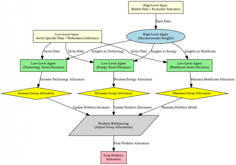
The IPS framework employs a MARL [7] approach to handle complex financial decision-making under dynamic and uncertain conditions. The architecture includes two types of agents: The high-level agent, which analyzes macroeconomic trends and provides strategic insights and the Low-Level agents that manage sector-specific asset groups, balancing group performance with overall portfolio objectives. The overall architecture of this system is illustrated in Figure 1.
Figure 1. The IPS framework with the high-level agent generating macroeconomic insights and the three low-level agents managing sector-specific decisions for portfolio allocation and rebalancing
3.1 Hierarchical agent structure and decision making
The hierarchical structure of the IPS system is modeled using the Hierarchical Markov Decision Process (HMDP) framework, a formal extension of the standard MDP applied in Hierarchical Reinforcement Learning (HRL) [18]. HMDPs have been widely used to capture multi-level temporal abstraction in decision-making processes by decomposing a global policy into sub-policies at different hierarchies of control [19]. In this formulation, each decision-making level corresponds to a semi-Markov process operating at its own temporal resolution. The high-level policy selects abstract actions (e.g., strategic allocations), which invoke lower-level policies that carry out more granular decisions (e.g., asset reallocations). In our framework, the high-level agent operates over a slower time scale and captures macroeconomic signals to make strategic portfolio-level decisions. In contrast, low-level agents act more frequently within their group-specific environments, executing sectoral or asset-level actions that refine the high-level strategy. Formally, each agent solves an MDP defined by the tuple ⟨S, A, P, R, γ⟩, with state and action spaces tailored to its decision level. The high-level agent uses macroeconomic state space Smacro and action space Amacro, while low-level agents operate over group-specific spaces Sgroup and Agroup. The overall IPS policy is modeled as a joint hierarchical policy:
$\begin{gathered}\pi\left(s_t\right)=\pi^{\text {macro}}\left(a_t^{\text {macro}} \mid s_t^{\text {macro}}\right). \\ \pi^{\text {group}}\left(a_t^{\text {group}} \mid s_t^{\text {group}}, a_t^{\text {macro}}\right)\end{gathered}$ (2)
This formulation ensures coordinated decision-making across both strategic and operational levels, enabling the IPS to integrate macroeconomic insights with sector-specific portfolio actions.
3.1.1 High-level agent: Macro-economic signal processing
The high-level agent in the IPS framework uses PPO [20] to update its policy in a stable and reliable manner. PPO constrains the magnitude of policy updates while maximizing long-term returns, making it well-suited for financial environments where overreaction to short-term changes can be costly. The PPO algorithm aims to maximize the following objective:
$\begin{gathered}L^{P P O}\left(\theta^{macro}\right) =\mathbb{E}_t\left[\min \left(r_t\left(\theta^{macro}\right) A_t^{macro}, clip\left(r_t\left(\theta^{macro}\right), 1\right.\right.\right. \left.\left.-\varepsilon, 1+\varepsilon) A_t^{macro}\right)\right]\end{gathered}$ (3)
The high-level agent provides strategic guidance for group-level portfolio adjustments, enabling hierarchical coordination with:
Inputs: The high-level agent processes macroeconomic indicators $X_t^{macro}$, including economic and market signals and global events influencing market movements.
Reward Function: Designed to balance risk-adjusted returns, portfolio stability, sectoral performance, and leverage management. The reward function incentivizes decisions aligned with market conditions. It integrates:
$R_t^{macro}=\alpha \cdot S R_t+\beta \cdot R_t^{stability}+\gamma \cdot S_t^{sector}-\delta \cdot L_t$ (4)
where, SRt is the Sharpe Ratio, calculated as:
$S R_t=\frac{\mathbb{E}\left[R_t\right]-R_f}{\sigma_t}$ (5)
here, $\mathbb{E}\left[R_t\right]$ is the expected return, $R_f$ is the risk-free rate, and $\sigma_t$ is the standard deviation of returns.
$R_t^{stability}$: The stability term, defined as the inverse of portfolio volatility:
$R_t^{stability}=\frac{1}{\sigma_t}$ (6)
This term rewards agents for maintaining a stable portfolio with lower volatility.
$S_t^{sector}$: Sector-specific Sharpe Ratios, which measure the performance of capital allocation to individual sectors. This term rewards effective sector allocation based on macroeconomic conditions, such as increasing exposure to defensive sectors during market downturns.
Lt: The leverage ratio, representing the extent of portfolio leverage. A penalty term is included to discourage excessive leverage during volatile markets.
The parameters α, β, γ, and δ control the relative importance of each component in the reward function, enabling the system to adapt its priorities dynamically. This reward function aims to ensure that high-level agents optimize portfolio strategies across macroeconomic, stability, sectoral, and leverage dimensions.
Actions: The high-level agent interprets macroeconomic signals to guide portfolio adjustments, including: Adjusting risk exposure (risk-on/risk-off), reallocating capital across asset classes, setting sectoral preferences, and modifying leverage ratios to adapt to market trends.
3.1.2 Low-level agents: group-level signal processing
In the IPS framework, each sector is managed by a dedicated low-level agent, which processes sector-specific signals to capitalize on shared market characteristics and optimize decision-making at a granular level. These agents are specialized to exploit common dynamics within their respective sectors, allowing IPS to adapt granularly to sectoral trends while aligning with overarching macroeconomic strategies.
Technology Sector Agent: The low-level agent for the technology sector focuses on high-growth opportunities, targeting assets with significant potential for value growth. This agent specializes in navigating the inherent volatility of the sector by optimizing asset allocation within subsectors such as semiconductors, cloud computing, and artificial intelligence.
Healthcare Sector Agent: The healthcare sector agent prioritizes stability and defensive performance, particularly during periods of economic uncertainty. This agent focuses on assets such as pharmaceutical companies and biotechnology firms, which are known for their resilience during market downturns.
Energy Sector Agent: The energy sector agent is tailored to manage the cyclical nature of this industry, focusing on macroeconomic indicators such as oil prices and geopolitical trends. This agent dynamically adjusts allocations within the sector to capitalize on market cycles.
To guide their decision-making, these agents rely on:
Inputs: These agents receive sector-specific inputs, including aggregated Open, High, Low, Close, Volume (OHLCV) market data and technical signals that capture trends and momentum for all assets within its assigned sector. This input structure enables low-level agents to refine their decisions based on sector-specific factors, while aligning their actions with the strategic guidance provided by the high-level agent.
Reward Function: The reward function for low-level agents in the IPS framework is designed to optimize sector-level decisions by balancing risk and growth objectives. The reward for a low-level agent managing a specific sector, Ri, is calculated as:
$R_i=\omega_i^{\text {risk }} \cdot \frac{E\left[R_i\right]}{\sigma_i}+\omega_i^{\text {growth }} \cdot \lambda \cdot C_i$ (7)
where, $\omega_i^{\text {risk}}:$ A weighting parameter that determines the emphasis on risk-adjusted returns; $\frac{E\left[R_i\right]}{\sigma_i}$: The Sharpe Ratio, representing the expected return $E\left[R_i\right]$ per unit of risk (volatility $\left.\sigma_i\right) ; \omega_i^{\text {growth}}$: A weighting parameter that prioritizes growth-focused objectives; λ: A growth scaling factor that controls the contribution of growth metrics to the reward function; Ci: A growth-oriented measure, such as capital allocation to high-potential sectors or industries.
Actions: Based on the received signals and computed rewards, each low-level agent undertakes sector-specific actions, such as adjusting portfolio weights for its assigned sector, reallocating resources among sector-specific assets, and managing exposure within the sector. These actions directly influence the portfolio's structure by optimizing risk and return within the agent’s assigned sector, while adhering to the guidelines set by the high-level agent.
This architecture ensures that low-level agents respond precisely to sector-specific dynamics while remaining synchronized with the strategic guidance of the high-level agent, enabling fine-grained control and improved portfolio coherence.
3.2 Bayesian neural networks for risk assessment in IPS
In the IPS framework, BNNs [11] are integrated into both the policy and value networks of each PPO agent, replacing deterministic neural networks. BNNs model epistemic uncertainty by treating network parameters as probability distributions rather than fixed values, allowing agents to avoid overconfident decisions in volatile financial environments.
Mathematically, this is formalized through Bayes’ theorem, where a prior distribution $p(\theta)$ over network weights is updated with data D to produce a posterior:
$p(\theta \mid D)=\frac{p(D \mid \theta) p(\theta)}{p(D)}$ (8)
To implement this in practice, we use Monte Carlo Dropout (MC Dropout) as an approximation to Bayesian inference, following [21]. During training and inference, dropout is applied at each forward pass, and multiple stochastic passes are used to estimate predictive distributions. The prior is implicitly defined by a Bernoulli distribution from the dropout mask, while the posterior is approximated using variational inference with stochastic gradient descent.
Although BNNs introduce additional computational overhead (approximately 1.5×compared to deterministic networks), this cost is justified by their ability to improve risk-aware decision-making and robustness in uncertain market conditions.
3.3 Attention-based communication for agent coordination in IPS
In many standard MARL frameworks, agents operate independently based only on local observations, without explicitly accounting for broader system-level information. While this may work in simple environments, financial markets are complex, dynamic systems with interdependent signals — such as macroeconomic indicators, sector-level trends, and correlated asset movements. Without effective inter-agent communication, agents risk missing broader market contexts, leading to suboptimal portfolio decisions.
To address this, the IPS architecture integrates agent-specific attention mechanisms that enable selective information exchange and prioritization. For the high-level agent, inputs include macroeconomic indicators such as GDP growth, interest rates, and global indices. For low-level agents, inputs consist of sector-specific OHLCV data and technical indicators. To enable selective communication, each agent first linearly projects its input feature vector X into query (Q), key (K), and value (V) representations using learned weight matrices:
$Q=W_Q \cdot X, K=W_k \cdot X, V=W_v \cdot X$ (9)
During communication, each agent ai receives its own observation oi and shared signals xj from other agents. The attention mechanism computes relevance scores eij using the scaled dot-product:
$e_{i j}=\frac{q_i \cdot k_j}{\sqrt{d}}$ (10)
These scores are normalized using the Softmax function to produce attention weights:
$a_{i j}=\frac{\exp \left(e_{i j}\right)}{\sum_{k=1}^n \exp \left(e_{i k}\right)}$ (11)
Finally, the context vector ci, which represents the weighted aggregation of shared signals, is computed as:
$c_i=\sum_{j=1}^n a_{i j} v_j$ (12)
where, vj=wvxj is the value vector derived from xj.
3.4 Hyperparameter optimization in IPS
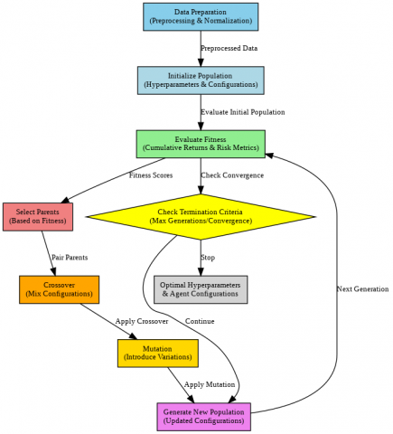
In IPS, hyperparameters are dynamically adjusted using GAs, which are well-suited for exploring high-dimensional spaces, avoiding local optima, and accommodating both continuous and discrete parameter types (Figure 2).
GAs optimize hyperparameters such as learning rates, discount factors, and sector-specific allocations by encoding them into chromosomes.
The GA workflow includes:
1. Initialization: Generating an initial population of candidate solutions (chromosomes).
2. Fitness Evaluation: Evaluating each chromosome using cumulative returns and risk-adjusted metrics.
3. Selection, Crossover, and Mutation: Selecting top-performing chromosomes, combining traits via crossover, and introducing mutations to maintain diversity and avoid local optima.
4. Iteration and Convergence: Repeating these steps until a termination criterion is met.
Table 1 presents possible hyperparameter settings for high-level and low-level agents in IPS.
Figure 2. Integration of genetic algorithms in the IPS system for agent configuration and optimization
Table 1. Possible hyperparameter settings for high-level and low-level agents in IPS
|
Agent Type |
Hyperparameter |
Range/Options |
Description |
|
High-Level Agent |
Learning Rate |
0.001 – 0.1 |
Controls the step size during optimization. |
|
Discount Factor |
0.9 – 0.99 |
Determines the importance of future rewards. |
|
|
Exploration Rate |
0.1 – 0.5 |
Probability of exploring new actions. |
|
|
Batch Size |
16, 32, 64, 128 |
Number of samples processed before updating. |
|
|
Epochs |
100 – 300 |
Number of complete passes through the dataset. |
|
|
Regularization (L2) |
0.0001 – 0.01 |
Reduces overfitting by penalizing large weights. |
|
|
Low-Level Agent |
Learning Rate |
0.001 – 0.1 |
Controls the step size during optimization. |
|
Discount Factor |
0.8 – 0.95 |
Determines the importance of future rewards. |
|
|
Exploration Rate |
0.1 – 0.5 |
Probability of exploring new actions. |
|
|
Batch Size |
16, 32, 64 |
Number of samples processed before updating. |
|
|
Epochs |
50 – 200 |
Number of complete passes through the dataset. |
|
|
Dropout Rate |
0.1 – 0.5 |
Probability of dropping units during training. |
4.1 Dataset overview
The IPS is evaluated using historical data from three major equity indices - S&P 500 [22], DAX [23] and FTSE 100 [24] - spanning January 2010 to June 2020. This diversified dataset includes 60 assets distributed across sectors, with 20 assets from the technology sector sourced from the S&P 500 and DAX, including semiconductors, software, and cloud computing. Another 20 assets belong to the healthcare sector, encompassing pharmaceutical companies, biotechnology firms, and healthcare equipment providers from all indices. The remaining 20 assets are from the energy sector, drawn from the FTSE 100 and DAX.
Each asset was allocated an initial investment of \$16,666.67 from a \$1,000,000 portfolio. The training period from 2010 to 2018 enabled the IPS to learn historical patterns, while the testing phase focused on two key periods: the pre-COVID era (2019–2020), characterized by stable market conditions for baseline evaluation, and the COVID-19 period (March–June 2020), serving as a stress test under extreme market volatility.
4.2 Dataset preprocessing
To prepare the dataset for the IPS, a combination of normalization and handling of missing data was applied. Min-max scaling was used to rescale feature values to a range between 0 and 1, ensuring consistency across all features. Missing values were addressed using forward and backward fill techniques to maintain continuity in the time series data. For training the IPS system, the hardware configuration included an Nvidia Tesla V100 GPU with 16 GB VRAM to handle deep learning tasks, an Intel Xeon Gold 6248 CPU with 20 cores and a clock speed of 2.5 GHz for auxiliary tasks and parallelized operations, 64 GB of DDR4 RAM for efficient data handling, and a 1 TB SSD for rapid data retrieval. In the implementation we utilize PyTorch for Bayesian Neural Networks, TensorFlow for attention mechanisms, and DEAP (Distributed Evolutionary Algorithms in Python) for optimizing Genetic Algorithms.
Table 2. Optimized hyperparameters using GA in Pre-COVID scenario
|
Agent Type |
Hyperparameter |
Range/Options |
|
High-Level Agent |
Learning Rate |
0.01 |
|
Discount Factor |
0.95 |
|
|
Exploration Rate |
0.3 |
|
|
Batch Size |
64 |
|
|
Epochs |
200 |
|
|
Regularization (L2) |
0.001 |
|
|
Low-Level Agent |
Learning Rate |
0.005 |
|
Discount Factor |
0.9 |
|
|
Exploration Rate |
0.4 |
|
|
Batch Size |
32 |
|
|
Epochs |
150 |
|
|
Dropout Rate |
0.2 |
Table 3. Optimized hyperparameters using GA in COVID scenario
|
Agent Type |
Hyperparameter |
Range/Options |
|
High-Level Agent |
Learning Rate |
0.005 |
|
Discount Factor |
0.85 |
|
|
Exploration Rate |
0.5 |
|
|
Batch Size |
64 |
|
|
Epochs |
150 |
|
|
Regularization (L2) |
0.001 |
|
|
Low-Level Agent |
Learning Rate |
0.002 |
|
Discount Factor |
0.85 |
|
|
Exploration Rate |
0.5 |
|
|
Batch Size |
32 |
|
|
Epochs |
120 |
|
|
Dropout Rate |
0.3 |
4.3 Experiment setup
4.3.1 GA-optimized configuration
The optimized hyperparameters for the IPS framework, obtained via GA tuning, are detailed in Table 2 (Pre-COVID) and Table 3 (COVID).
The GA-optimized configurations were tailored to the distinct Pre-COVID and COVID scenarios:
Higher Dropout and Exploration Rates: In the COVID scenario, the dropout rate increased from 0.2 to 0.3 and the exploration rate from 0.4 to 0.5, mitigating overfitting and encouraging agents to explore diverse strategies in volatile conditions.
Adjusted Learning Rates and Discount Factors: Learning rates for high- and low-level agents were reduced to 0.005 and 0.002, respectively, to stabilize training in volatile markets. Lower discount factors placed greater emphasis on short-term rewards, aligning with rapidly changing market conditions.
4.3.2 Evaluation metrics
The IPS's performance was evaluated using key metrics to quantify risk and return, including Total Return, Sharpe Ratio, Maximum Drawdown, Sortino Ratio, and Volatility.
4.3.3 Testing configurations
Four configurations were tested to assess IPS effectiveness:
Single-Agent PPO: A baseline model using standard neural networks (NNs) and manually tuned hyperparameters, serving as a comparison point for advanced configurations.
Multi-Agent PPO with NNs: Introduces multiple agents, each managing a specific sector (Technology, Healthcare, Energy) using PPO with standard NNs. This configuration isolates the benefits of multi-agent systems without uncertainty modeling.
Multi-Agent PPO with BNNs: This configuration applies BNNs within a multi-agent PPO setup. It serves to assess the isolated impact of uncertainty modeling on portfolio optimization.
IPS System: Features multiple agents using PPO with BNNs for uncertainty modeling, enhanced with Genetic Algorithms for dynamic hyperparameter tuning.
4.3.4 Traditional baseline strategies
To broaden the benchmarking scope beyond reinforcement learning methods, two traditional portfolio optimization strategies were implemented:
Risk Parity: Allocates capital such that each asset contributes equally to the overall portfolio risk. It is widely used in institutional portfolio management for balanced risk exposure.
Minimum Variance Portfolio: Constructs a portfolio that minimizes overall return volatility by optimizing asset weights based on their covariances.
These models were implemented using the PyPortfolioOpt library and evaluated over the same datasets and timeframes as the RL-based configurations to ensure fair comparisons.
4.4 Results
4.4.1 Performance during stable markets (Pre-COVID)
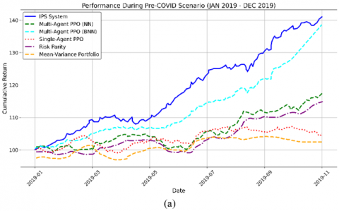
During the Pre-COVID period (January 2019 – December 2019), the IPS system achieved the highest cumulative return, reaching nearly 40%, clearly outperforming all other strategies. Figure 3 illustrates this gap visually, showing that IPS maintained a steep and steady growth trajectory, while competing strategies lagged behind—especially Single-Agent PPO and traditional baselines like Risk Parity and Mean Variance Portfolio, which flattened early in the period.
Table 4 complements this by reporting detailed metrics, where IPS achieved the highest Sharpe Ratio (1.25) and Sortino Ratio (1.55), reflecting strong risk-adjusted performance. Its Maximum Drawdown of −4.5% was also the lowest across all methods, confirming superior downside protection. Moreover, the IPS system maintained the lowest volatility (4.2%), reinforcing its stability during this calm market phase.
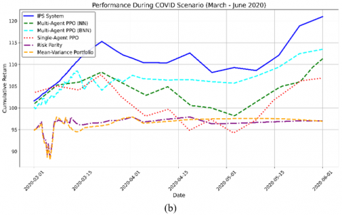
Figure 3. Cumulative return for single-agent PPO, multi-agent PPO (NN), multi-agent PPO (BNN), IPS, Risk Parity, and Mean Variance Portfolio in (a) Pre-COVID and (b) COVID scenarios
Table 4. Performance metrics comparison for single-agent PPO, multi-agent PPO (NN), multi-agent PPO (BNN), IPS, Risk Parity, and Mean Variance Portfolio in Pre-COVID and COVID scenarios
|
Metric |
Single-Agent PPO |
Multi-Agent PPO (NN) |
Multi-Agent PPO (BNN) |
IPS |
Risk Parity |
Mean Variance Portfolio |
|
Pre-COVID |
||||||
|
Sharpe Ratio |
1.02 |
1.15 |
1.21 |
1.25 |
1.02 |
1.15 |
|
Maximum Drawdown (%) |
-7.8 |
-6.3 |
-5.2 |
-4.5 |
-7.8 |
-6.3 |
|
Sortino Ratio |
1.25 |
1.40 |
1.52 |
1.55 |
1.25 |
1.40 |
|
Volatility (%) |
4.6 |
4.8 |
4.4 |
4.2 |
4.6 |
4.8 |
|
COVID |
||||||
|
Sharpe Ratio |
0.55 |
0.62 |
0.71 |
0.78 |
0.55 |
0.62 |
|
Maximum Drawdown (%) |
-20.5 |
-15.3 |
-12.3 |
-10.2 |
-20.5 |
-15.3 |
|
Sortino Ratio |
0.65 |
0.75 |
0.88 |
0.95 |
0.65 |
0.75 |
|
Volatility (%) |
15.8 |
14.5 |
13.4 |
12.8 |
15.8 |
14.6 |
4.4.2 Performance during volatile markets (COVID-19)
During the COVID-19 market shock (March–June 2020), the IPS system consistently outperformed all baseline strategies, achieving a peak cumulative return of approximately 20%, clearly ahead of multi-agent PPO (BNN) with ~15%, PPO (NN) with ~10%, and Single-Agent PPO with ~5%. As shown in Figure 3, the IPS curve maintains steady growth, while other strategies—particularly Risk Parity and Mean-Variance—flatten or decline during high-volatility periods. In contrast, Risk Parity and Mean-Variance Portfolio exhibited subdued performance, which reflects their conservative nature during high-stress conditions.
Statistical analysis supports these observations, as detailed in Table 4. The IPS recorded the highest Sharpe Ratio (0.78) and Sortino Ratio (0.95), indicating the best risk-adjusted returns in this volatile regime. Notably, it also achieved the lowest Maximum Drawdown (−10.2%), compared to −12.3% for multi-agent PPO (BNN), and much deeper losses for standard PPO and traditional portfolios.
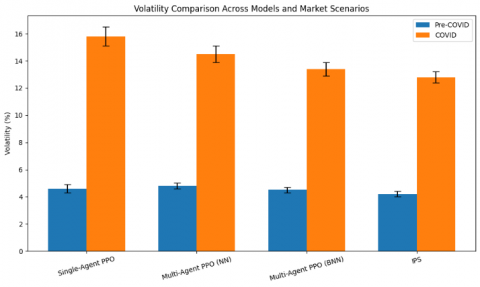
The Volatility metric, also reported in Table 4, confirms IPS's stability, with the lowest observed value at 12.8%, highlighting its effective risk management and adaptability.
Risk Parity and Mean-Variance strategies, though traditionally stable, experienced notable short-term fluctuations (as seen in Figure 3), validating the realism of market reaction. However, their performance remained limited, with Sharpe Ratios of 0.55 and 0.62, respectively, and drawdowns reaching −20.5% and −15.3%.
4.4.3 Sector-specific performance
The IPS system’s hierarchical architecture enabled each low-level agent to contribute to portfolio performance with specialized sector strategies. This is quantitatively confirmed in Table 5, which reports the Sharpe Ratio, Maximum Drawdown, and Volatility across all three sectors (Technology, Healthcare, and Energy) during both the Pre-COVID and COVID periods. These sector-specific results highlight how each agent adapted to distinct market dynamics.
Table 5. Performance of sector agents (Technology, Healthcare, Energy) in Pre-COVID and COVID scenarios
|
Sector |
Period |
Sharpe Ratio |
Maximum Drawdown (%) |
Volatility (%) |
|
Technology |
Pre-COVID |
1.35 |
-5.0 |
4.5 |
|
COVID |
0.80 |
-12.0 |
6.0 |
|
|
Healthcare |
Pre-COVID |
1.50 |
-4.0 |
4.0 |
|
COVID |
1.25 |
-3.5 |
4.2 |
|
|
Energy |
Pre-COVID |
1.10 |
-6.0 |
7.5 |
|
COVID |
0.70 |
-8.5 |
7.5 |
Technology Sector Performance: In the technology sector, the agent capitalized on growth opportunities during the Pre-COVID period, achieving a Sharpe Ratio of 1.35, a Maximum Drawdown of –5.0%, and volatility of 4.5%. During the COVID period, the agent shifted to more risk-averse strategies, reducing exposure to volatile assets, resulting in a Sharpe Ratio of 0.80 and a Maximum Drawdown of -12.0%.
Healthcare Sector Performance: The healthcare agent adopted a defensive posture, prioritizing stability during the Pre-COVID period and achieving the highest Sharpe Ratio (1.50). During COVID, the agent maintained its risk-averse stance, achieving a Sharpe Ratio of 1.25, a Maximum Drawdown of –3.5%, and the lowest volatility (4.0%). These values confirm the Healthcare sector’s stabilizing effect, especially during turbulent periods.
Energy Sector Performance: The energy agent demonstrated cyclical adaptability. It achieved a Sharpe Ratio of 1.10 and a Maximum Drawdown of –6.0% Pre-COVID. During COVID, it reallocated toward renewable assets to mitigate losses, resulting in a Sharpe Ratio of 0.70, a Maximum Drawdown of –8.5%, and Volatility of 7.5%.
4.5 Discussion
Table 4 and Figure 3 demonstrate that the IPS system consistently outperformed all baseline strategies across both stable (Pre-COVID) and turbulent (COVID-19) market conditions. It achieved the highest cumulative returns, superior risk-adjusted metrics, and the lowest drawdowns and volatility. These results validate the effectiveness of IPS’s hierarchical architecture, uncertainty-aware modeling, and dynamic coordination mechanisms.
Table 5 further illustrates how attention-based communication and hierarchical policy decomposition enabled sector-specific agents to specialize and adapt their strategies. For example, the Technology agent drove portfolio growth during the Pre-COVID period, achieving a Sharpe Ratio of 1.35, while adopting a more risk-averse stance during COVID-induced volatility. The Healthcare agent provided consistent defensive strength, recording the lowest volatility (4.0%) pre-COVID and the lowest drawdown (−3.5%) during COVID. Meanwhile, the Energy agent dynamically reallocated toward renewable assets in response to shifting demand. These sector-level behaviors highlight the advantages of decentralized control and agent specialization in volatile environments.
Compared to the single-agent PPO baseline, multi-agent PPO consistently demonstrated better performance across risk and return metrics, confirming the value of decentralized decision-making. Multi-agent architectures enable collaboration among agents, which enhances responsiveness to heterogeneous market signals and improves portfolio robustness in dynamic financial settings (Table 4 and Figure 3).
A key contributor to IPS’s superior performance is the integration of Bayesian Neural Networks (BNNs) and attention mechanisms. BNNs enabled probabilistic forecasting by modeling epistemic uncertainty, helping agents avoid overconfident decisions under noisy or limited data. In parallel, attention modules allowed agents to prioritize critical macroeconomic and sector-specific inputs, improving both coordination and precision in action selection. During the COVID-19 period, the IPS achieved a Sharpe Ratio of 0.78 and volatility of 12.8%, significantly outperforming the multi-agent PPO with deterministic NNs (Sharpe Ratio: 0.62, Volatility: 14.5%) and even the BNN-based PPO without attention or hierarchy (Sharpe Ratio: 0.71, Volatility: 13.4%)—as shown in Table 4 and Figure 4.
This trend of performance enhancement was consistent across both market regimes. During the Pre-COVID period, the IPS achieved the highest Sharpe Ratio (1.25) and the lowest drawdown (−4.5%), compared to 1.21 and −5.2% for the BNN-based PPO and 1.15 and −6.3% for the deterministic PPO. These results demonstrate the incremental value of each architectural enhancement in the IPS pipeline.
Importantly, this structured comparative analysis directly addresses the role of BNNs in the IPS system. The stepwise performance gains from Multi-Agent PPO with deterministic NNs → BNNs → full IPS confirm the value of incorporating uncertainty modeling. BNNs significantly enhance the robustness, risk sensitivity, and generalization capabilities of the IPS framework under both normal and stress-test conditions.
4.6 Statistical significance analysis
To account for the stochastic nature of both financial markets and reinforcement learning algorithms, we conducted a statistical validation of all experimental results. Each configuration—single-agent PPO, multi-agent PPO with standard neural networks (NN), multi-agent PPO with BNN, and the proposed IPS system—was trained and evaluated over 10 independent runs, each initialized with a different random seed to ensure robustness.
For each run, we recorded the Sharpe Ratio, Maximum Drawdown, and Volatility during both the Pre-COVID and COVID periods. We report the results as mean ± standard deviation to reflect performance consist&ency across trials.
As shown in Table 6, the IPS system consistently achieved statistically superior performance across all key metrics. For instance, during the COVID-19 period, IPS reached a Sharpe Ratio of 0.78 ± 0.04, outperforming multi-agent PPO (BNN) at 0.70 ± 0.04, multi-agent PPO (NN) at 0.62 ± 0.05, and Single-Agent PPO at 0.55 ± 0.07. Similarly, IPS recorded a lower Maximum Drawdown (−10.2% ± 0.5%) and lower Volatility (12.8% ± 0.4%), demonstrating superior downside protection and robustness under extreme conditions.
Table 6. Comparative performance of PPO variants using statistical metrics (Mean ± SD) in Pre-COVID and COVID scenarios
|
Metric |
Scenario |
SingleAgent PPO |
Multi-Agent PPO (NN) |
Multi-Agent PPO (BNN) |
IPS |
|
Sharpe Ratio |
Pre-COVID |
1.02 ± 0.06 |
1.15 ± 0.05 |
1.20 ± 0.04 |
1.25 ± 0.04 |
|
COVID |
0.55 ± 0.07 |
0.62 ±0.05 |
0.70 ± 0.04 |
0.78 ± 0.04 |
|
|
Max Drawdown (%) |
Pre-COVID |
-7.8 ± 0.6 |
-6.3 ±0.5 |
-5.2 ± 0.4 |
-4.5 ± 0.3 |
|
COVID |
-20.5 ± 0.8 |
-15.3 ± 0.7 |
-12.0 ± 0.6 |
-10.2 ± 0.5 |
|
|
Volatility (%) |
Pre-COVID |
4.6 ± 0.3 |
4.8 ± 0.2 |
4.5 ± 0.2 |
4.2 ± 0.2 |
|
COVID |
15.8 ± 0.7 |
14.5± 0.6 |
13.4 ± 0.5 |
12.8 ± 0.4 |
These trends were also observed during stable market conditions in the Pre-COVID period, where IPS maintained the highest Sharpe Ratio (1.25 ± 0.04) and the lowest drawdown (−4.5% ± 0.3%) among all methods.
Visual comparisons in Figures 4–6 further reinforce these findings. Each chart includes error bars representing standard deviation, clearly illustrating the consistency and reliability of the IPS system. The performance differences are not attributable to random variation, but instead arise from the system’s architectural innovations—notably, the integration of BNNs, attention mechanisms, and hierarchical reinforcement learning.
These results confirm that IPS delivers statistically robust improvements in both stable and volatile regimes, and substantiate the model’s effectiveness beyond pointwise performance.
Figure 4. Sharpe ratio comparison across portfolio optimization models and market conditions
Figure 5. Volatility comparison across portfolio optimization models and market conditions
Figure 6. Maximum drawdown comparison across portfolio optimization models and market conditions
In this study, we introduced the IPS, a hierarchical reinforcement learning framework enhanced with BNNs, PPO, and attention mechanisms. The IPS demonstrated strong adaptability to varying market conditions, with high-level agents providing macroeconomic insights and low-level agents performing sector-specific optimization. This hierarchical design enabled coherent and context-aware decision-making across diverse financial scenarios.
Experimental results confirmed the IPS system’s superiority over single-agent and multi-agent PPO baselines using both deterministic neural networks and BNNs, as well as traditional risk-based strategies such as Risk Parity and the Minimum Variance Portfolio. While multi-agent PPO with BNNs already improved robustness and uncertainty modeling compared to deterministic approaches, the IPS system consistently achieved higher risk-adjusted returns, lower volatility, and reduced drawdowns, particularly during periods of extreme market turbulence such as the COVID-19 crisis. The integration of BNNs within the IPS framework enhanced its ability to capture uncertainty in financial environments, while attention mechanisms further improved inter-agent coordination and signal prioritization. Additionally, GAs contributed by dynamically optimizing hyperparameters, enabling the system to adapt effectively in both stable and volatile market conditions.
To further enhance the applicability of the IPS framework, future work will explore its performance across a more diverse set of global equity markets, including indices from Asia, Latin America, and Africa. This will allow us to assess the IPS system’s robustness and generalizability in financial environments that exhibit different structural dynamics, liquidity profiles, and volatility patterns compared to developed markets.
Additionally, we plan to benchmark the IPS framework against a wider range of state-of-the-art portfolio optimization strategies, such as transformer-based architectures, Bayesian ensemble models, and distributional reinforcement learning approaches. These comparisons will help position IPS within the broader ecosystem of advanced financial optimization systems.
Future enhancements will also incorporate real-time data sources, including sentiment analysis from social media and news, as well as explore more advanced reinforcement learning techniques such as distributed actor-critic methods. These efforts aim to increase the scalability, adaptability, and real-world applicability of the IPS framework.
[1] Shiller, R.J. (2005). Irrational Exuberance. 2nd ed. Princeton University Press, Princeton, USA.
[2] Elton, E.J., Gruber, M.J. (1995). Modern Portfolio Theory and Investment Analysis. Wiley, New York.
[3] Barberis, N., Shleifer, A., Wurgler, J. (2005). Comovement. Journal of Financial Economics, 75(2): 283-317. https://doi.org/10.1016/j.jfineco.2004.04.003
[4] Fama, E.F. (1970). Efficient capital markets. Journal of Finance, 25(2): 383-417. https://doi.org/10.2307/2325486
[5] Chib, P.S., Singh, P. (2023). Recent advancements in end-to-end autonomous driving using deep learning: A survey. IEEE Transactions on Intelligent Vehicles, 9(1): 103-118. https://doi.org/10.48550/arXiv.2307.0437
[6] Raza, S.M., Sajid, M., Singh, J. (2022). Vehicle routing problem using reinforcement learning: Recent advancements. In Advanced Machine Intelligence and Signal Processing, pp. 269-280. https://doi.org/10.1007/978-981-19-0840-8_20
[7] Zhang, K., Yang, Z., Başar, T. (2021). Multi-agent reinforcement learning: A selective overview of theories and algorithms. In Handbook of Reinforcement Learning and Control, pp. 321-384. https://doi.org/10.48550/arXiv.1911.10635
[8] Liu, Z., Chen, B., Zhou, H., Koushik, G., Hebert, M., Zhao, D. (2020). Mapper: Multi-agent path planning with evolutionary reinforcement learning in mixed dynamic environments. In 2020 IEEE/RSJ International Conference on Intelligent Robots and Systems (IROS), Las Vegas, NV, USA, pp. 11748-11754. https://doi.org/10.1109/IROS45743.2020.9340876
[9] Pu, Y., Li, F., Rahimifard, S. (2024). Multi-agent reinforcement learning for job shop scheduling in dynamic environments. Sustainability, 16(8): 3234. https://doi.org/10.3390/su16083234
[10] Zhang, H., Li, J., Qi, Z., Aronsson, A., Bosch, J., Olsson, H.H. (2023). Multi-agent reinforcement learning in dynamic industrial context. In 2023 IEEE 47th Annual Computers, Software, and Applications Conference (COMPSAC), Torino, Italy, pp. 448-457. https://doi.org/10.1109/COMPSAC57700.2023.00066
[11] MacKay, D.J.C. (1992). Bayesian Learning for Neural Networks. Springer, New York. https://doi.org/10.1007/978-1-4612-0745-0
[12] Ngartera, L., Issaka, M.A., Nadarajah, S. (2024). Application of bayesian neural networks in healthcare: Three case studies. Machine Learning and Knowledge Extraction, 6(4): 2639-2658. https://doi.org/10.3390/make6040127
[13] Thakur, S., van Hoof, H., Higuera, J.C.G., Precup, D., Meger, D. (2019). Uncertainty aware learning from demonstrations in multiple contexts using bayesian neural networks. In 2019 International Conference on Robotics and Automation (ICRA), Montreal, QC, Canada, pp. 768-774. https://doi.org/10.1109/ICRA.2019.8794328
[14] Li, C., Jiang, J., Zhao, Y., Li, R., Wang, E., Zhang, X., Zhao, K. (2022). Genetic algorithm based hyper-parameters optimization for transfer convolutional neural network. In International Conference on Advanced Algorithms and Neural Networks (AANN 2022), Zhuhai, China, pp. 232-241. https://doi.org/10.1117/12.2637170
[15] Xiao, X., Yan, M., Basodi, S., Ji, C., Pan, Y. (2020). Efficient hyperparameter optimization in deep learning using a variable length genetic algorithm. arXiv Preprint arXiv:2006.12703. https://doi.org/10.48550/arXiv.2006.12703
[16] Rachev, S.T., Racheva-Iotova, B., Stoyanov, S.V., Fabozzi, F.J. (2010). Risk management and portfolio optimization for volatile markets. In Handbook of Portfolio Construction, pp. 493-508. https://doi.org/10.1007/978-0-387-77439-8_17
[17] Markowitz, H. (1952). Portfolio Selection. The Journal of Finance, 7(1): 77-91. https://doi.org/10.2307/2975974
[18] Sutton, R.S., Barto, A.G. (2018). Reinforcement Learning: An Introduction. 2nd ed. MIT Press, Cambridge.
[19] Dietterich, T.G. (2000). Hierarchical reinforcement learning with the MAXQ value function decomposition. Journal of Artificial Intelligence Research, 13: 227-303. https://doi.org/10.1613/jair.639
[20] Schulman, J., Wolski, F., Dhariwal, P., Radford, A., Klimov, O. (2017). Proximal policy optimization algorithms. arXiv Preprint arXiv:1707.06347. https://doi.org/10.48550/arXiv.1707.06347
[21] Gal, Y., Ghahramani, Z. (2016). Dropout as a Bayesian approximation: Representing model uncertainty in deep learning. arXiv Preprint arXiv:1506.02142. https://doi.org/10.48550/arXiv.1506.02142
[22] Yahoo Finance – Stock Market Live, Quotes, Business & Finance News. https://finance.yahoo.com/, accessed on 5 Feb. 2025.
[23] Investing.com – Stock Market Quotes & Financial News. https://www.investing.com/, accessed on 5 Feb. 2025.
[24] Bloomberg Middle East. https://www.bloomberg.com/middleeast, accessed on 5 Feb. 2025.