Yasser Khaddor*![]() | Abdes Samed Bernoussi
| Abdes Samed Bernoussi![]() | Mohamed Byari
| Mohamed Byari![]()
© 2025 The authors. This article is published by IIETA and is licensed under the CC BY 4.0 license (http://creativecommons.org/licenses/by/4.0/).
OPEN ACCESS
Traditional methods for modeling heat transfer in the building envelope often struggle to capture complex geometries and include material heterogeneity. In this work, we introduce a novel approach combining mathematical modeling through cellular automata (CA) with geometrical capturing through light detection and ranging (LiDAR) to analyse the thermal performance of building facades. Physical data for the model are collected using LiDAR scanning, which provides precise digital representations of facade geometry and captures structural complexity, and CA modeling is used to simulate heat transfer, accounting for variations in material properties and detailed geometric features. We applied the model to a real building in Northern Morocco, the results showed the effecet of shading on reducing energy loads of the building. The model was evaluated using infrared thermal imaging. By integrating LiDAR as a data acquisition tool with mathematical and computational methods, this approach offers a robust framework for evaluating the thermal performance of building facades.
CA, LiDAR scanning, heat transfer simulation, lattice
Buildings are considered one of the most consuming sectors in the global energy consumption [1], in order to improve their energy efficiency and reduce their carbon emissions, it’s essential to understand heat transfer dynamics in the building envelope [2]. Building envelopes are not considered just physical barriers, they are seen as dynamic systems that can interact with external environmental stressors like wind, solar exposure and outside temperature fluctuations, while ensuring inside comfort by controlling internal conditions [3]. Mathematical modeling of heat transfer in these systems plays a crucial role in advancing sustainable construction practices and reducing building energy consumption [4].
Methods for analyzing heat transfer in building envelopes can struggle with complexity factors, such as heterogeneous material properties, complex geometries, and advanced designs that use shading devices and high-performance materials [5-7]. Thus, we need more advanced computational techniques capable of handling such complexities.
With advancements in data acquisition technologies, such as terrestrial light detection and ranging (LiDAR), precise measurements can be obtained even with complex geometries [8-10]. LiDAR scans provide high-resolution point clouds that represent a detailed digital representation of buildings facades, this provides valuable inputs for computational simulations. LiDAR is used for thermal analysis, we find studies such as Wang et al. [11] demonstrated the integration of thermal data with LiDAR scans to create virtual representations of energy performance in existing buildings, providing a tool that can help in energy retrofit decisions. Similarly, projects like ThermalMapper [12] illustrate the potential of combining LiDAR with thermal imaging to enhance understanding of heat loss and energy performance in building envelopes. By generating accurate geometric data, LiDAR serves as a powerful tool to support thermal simulations [9].
Even with the availability of high-resolution geometrical data, these approaches have been limited to static assessments. Dynamic simulations of heat transfer across building facades remain a challenge due to the interplay of physical processes, varied material properties, and geometric irregularities [13]. Addressing these challenges requires advanced mathematical and computational models.
In this study, we introduce a novel simulation framework that combines mathematical modeling using cellular automata (CA) for computational simulations of heat transfer, using high-resolution LiDAR scans for data acquisition. CA has been used as modeling tool for ecological and socio-environmental applications [14-16]. They are particularly well suited for modeling complex systems [17] because they focus on localized interactions between discrete elements (cells) while preserving a global system perspective. For thermal analysis, CA have been applied due to their ability to capture complex heat transfer via local interaction rules [18, 19], offering computational efficiency over traditional methods. However, most studies using CA for thermal analysis use predefined networks, resulting in a lack of spatial accuracy. This can represent a limitation in thermal modeling using CA. Such a limitation can influence heat transfer dynamics, leading to inaccuracies, particularly when applied to heterogeneous surfaces with variations in material properties and geometries. In contrast to conventional CA approaches that operate on generalized spatial grids, the use of LiDAR-derived facade geometries and material-specific attributes enables a more accurate representation of heat flows on urban surfaces. Moreover, by combining the dynamic heat propagation capabilities of CA with the spatial accuracy of LiDAR, this approach overcomes the limitations of both methodologies. Compared to previous studies in which CA is used with simplified spatial inputs [20, 21] or using LiDAR for static thermal analysis, this work offers a more comprehensive modeling framework that improves predictive accuracy in building thermal performance assessments.
In this study, each cell in our CA model is assigned specific thermal properties such as conductivity, heat capacity, and density to simulate localized heat transfer processes with high accuracy.
A key innovation of our approach is in its integration of a 2.5-dimensional representation of building facades, generated from LiDAR scans along with CA modeling. This combination captures variations in facade geometry while maintaining computational efficiency. The framework effectively addresses the challenges of heterogeneity and complex geometries in real-world building materials, enabling detailed simulations of heat flow patterns. By identifying areas of significant thermal gain or loss, this approach provides insights that simpler models may overlook, contributing to more informed strategies for energy efficiency.
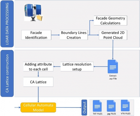
The proposed methodology as illustrated in Figure 1 begins with acquiring LiDAR point cloud data, which serves as our geometric information. Then we manually identify the facade within the point cloud, and define the boundary lines to clearly show the facade's limits. As a result, a 2D point cloud representation of the facade is generated by removing extraneous data points. We then use this cleaned data to refine the facade geometry.
Figure 1. Process of using lidar data points as input of the cellular automata multi-scale model
We adjust the resolution of the data to suit the required simulation. Then we assign material attributes to each point. This step enables the integration of material heterogeneity into our model. Finally, our lattice structure is constructed to represent the facade as input to our CA model, making it easier to simulate heat transfer dynamics.
2.1 Cellular automata generalities
CA is a discrete computational model where space, time, and state are all represented in discrete units [22]. The choice of CA over traditional numerical methods is mainly because of the balance CA strikes between computational efficiency, scalability, and accuracy in heat transfer modeling [23]. While finite element methods (FEMs) and finite volume methods offer high accuracy, their complex mesh and large systems of equations make them computationally prohibitive for large-scale facade simulations. CA operates on local interaction rules. Even with their simplicity, local rules allow complex spatial dependencies to be captured without the need for global information exchange [24] reducing complexity while maintaining spatial resolution.
A CA is defined by a quadruplet $A\left( \mathcal{L},\mathcal{N},S,f \right)$ with initial and boundary conditions, where $\mathcal{L}$ is a set of cells, $\mathcal{N}$ is the neighborhood system of cells, $S$ is the set of cell states, $f$ is the transition function of the cell state.
2.1.1 Lattice $\mathcal{L}$
The lattice $\mathcal{L}$ is a network consisting of cells $c$ arranged in a specific pattern. In our 2D model, cells can be arranged in rectangular or hexagonal shapes.
$L=\left\{ {{c}_{ij}}\ \text{ }\!\!|\!\!\text{ }\ i,j\in {{\mathbb{Z}}^{2}} \right\}$ (1)
2.1.2 Neighborhood $\mathcal{N}$
The neighborhood $\mathcal{N}\left( c \right)$ for a cell $c$ is the set of cells affecting its evolution. Different types of neighborhoods can be considered, such as von Neumann, Moore neighborhoods or uniform neighborhoods, see Figure 2.
Figure 2. Neighborhood types
In our model we use uniform neighborhood (Hexagonal Lattice): For a hexagonal lattice, each cell is affected by its six neighbors.
2.1.3 States set $S$
The set $S$ is finite and represents all possible states of each cell. States can be values, conditions, or other descriptors necessary to describe the evolution of the phenomenon.
$S=\left\{ {{s}_{1}},{{s}_{2}},\ldots ,{{s}_{k}} \right\},k=card\left( S \right)$ (2)
2.1.4 Attributes
To overcome the problem of modeling a complex phenomenon in the case of a heterogeneous medium where the cell state depends on several factors and properties that characterize the space. In this way, we consider that the cell can be associated with a set of space attributes. This approach introduced in reference [25] allows us to separate the state of the phenomenon and the space characteristics that impact it. The attributes are applications linking each cell to a static or dynamic space characteristic, defined by Eq. (3).
$\begin{matrix} \sigma : & \mathcal{L}\times I & \to & {{F}_{\sigma }} \\ {} & \left( {{c}_{ij}},{{t}_{\tau }} \right) & \mapsto & {{\sigma }^{{{t}_{\tau }}}}\left( {{c}_{ij}} \right) \\ \end{matrix}$ (3)
where, $\mathcal{L}$ is the lattice, $I$ is the time interval and ${{F}_{\sigma }}$ is a bounded set that represent all the possible value that could be taken by a cell attribute.
2.1.5 Transition rules $f$
The CA evolves in discrete time steps, where the state of a cell at time $t+1$ depends on its neighborhood at time $t$.
${{S}_{t+1}}=f\left( {{S}_{t}}\left( N\left( c \right) \right) \right)$ (4)
Transition function $f$ allows determining the state of a cell $c$ at an instant ${{t}_{\tau +1}}$ depending on its neighborhood state at an instant ${{t}_{\tau }}$.
2.2 LiDAR points processing
A manual pre-processing analysis was conducted to correct the data and convert the data into a 2D.xy format compatible with our model input format. Laser scanners, when capturing complex scenes, generate millions of points with high density and millimeter-level accuracy. To focus solely on the façade of interest, we filtered out extraneous environmental points. The data was transformed from 3D to 2D, representing the façade. The coordinates of the resulting point cloud were stored in a (.xyz) format file, which includes both spatial coordinates and the "RGB" color data of each point. We then exported the data set that enabled the construction of a cellular lattice with the same pixel size and adjustable resolution.
2.2.1 Lattice resolution
The choice of lattice resolution has a significant impact on the study of spatiotemporally evolving phenomena and computational resources. The choice of a low resolution significantly reduces the accuracy of the simulation and decreases the exchange of local information associated with each cell [26], making communication between these cells more complex, requires to build more complex transition rules.
Figure 3 is an illustration of lattice constructions from the same data collected from scanning a building. $card\left( \mathcal{L} \right)$ refers to the number of cells in the lattice. Three different resolution ratios are chosen. On ratio 1, is the direct number taken filtering unnecessary points from the lidar scan, it contains 901307 cells. As we increase the resolution ratio the number of cells decreases.
Figure 3. Illustration of different cell lattice resolutions from the same data collected of LiDAR scan
If the resolution ratio is low, the model will require more computational resources and extended processing time. Therefore, it is essential to strike a balance between resolution ratio and computational efficiency to select a lattice for the simulation. And that is done by selecting the right on ratio value (cell size).
The model describes the heat transfer phenomena in the building facades to simulate thermal dynamics and shading effects on a building facade.
3.1 Lattice
The lattice $\mathcal{L}$ represents a 2.5-dimensional space, where each cell corresponds to a section of the building facades. This space is discretized based on the LiDAR scan, which provides a highly detailed point cloud. Each cell in the lattice has associated material properties (e.g., thermal conductivity, heat capacity), which are essential for the simulation of heat transfer. The shape and arrangement of the cells are determined by the dimensions of the building and the geometric complexity captured by the scan. We define a cellular lattice by Eq. (5).
$\mathcal{L}=\left\{ {{c}_{i,j}} \right\};i,j\in \mathbb{Z}$ (5)
where, $i$ and $j$ represent spatial indices in two dimensions, with height variation considered as a parameter influencing heat exchange processes. The LiDAR point cloud data is interpolated to form the facade geometry, ensuring accurate representation of shading devices and surface undulations.
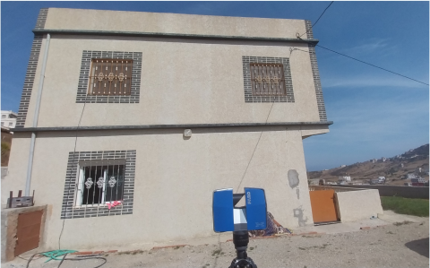
Figure 4 is a house located in Northern Morocco, constructed in 2017. This residence is situated near Dikki Beach in Tangier, an area known for a warm climate. The architectural design of this building reflects the local aesthetic, blending modern elements with traditional Moroccan styles. The lattice constructed from LiDAR scan, shown in Figure 5, is represented by a 2D array, made from a point cloud of 281 043 points.
Figure 4. Facade building image (Northen Morocco)
Figure 5. ExtracteLiDAR scan
3.2 Neighborhood
The neighborhood $N\left( c \right)$ of a cell $c$ defines the set of adjacent cells with which it interacts thermally. In this study, we use a uniform neighborhood, meaning that each cell interacts with its six surrounding neighbors in the horizontal plane, as well as neighboring cells in the vertical direction to account for facade depth variations.
This neighborhood structure allows for heat exchange in different directions, ensuring that the thermal interactions between various facade elements are captured accurately.
3.3 States
We define a range of hot, cold, and comfortable surface conditions based on the meteorological data of the studied region and the material properties of the surface. For instance, a surface considered cold in a hot climate may be perceived as comfortable in a colder climate. Taking into account these ranges, we consider these states:
$\left\{ \begin{array}{*{35}{l}} state~0:cold~surface: & If~{{T}_{0}}\le {{T}_{t}}\le {{T}_{1}} \\ state~1:comfort~surface & If~{{T}_{1}}<{{T}_{t}}\le {{T}_{2}} \\ state~3:hot~surface: & If~{{T}_{2}}<{{T}_{t}}\le {{T}_{3}} \\ \end{array} \right.$ (6)
The cell states encode information about the energy stored $Q$ and temperature distribution $T$. The choice of the number n and values of ${{T}_{i}}\left( 0\le i\le 3 \right)$ depend on the considered study case. State transition happened according to transition rules.
3.4 Attributes
Table 1 represents cells attributes considered in the model.
Table 1. Attribute set considered in model
|
Attribute |
Symbol |
Value Range |
|
Temperature |
T |
$\mathcal{L}\to \mathbb{R}$ |
|
Shading status |
S |
$\mathcal{L}\to \left[ 0,~1 \right]$ |
|
Thermal conductivity |
λ |
$\mathcal{L}\to \mathbb{R}^+$ |
|
Density |
ρ |
$\mathcal{L}\to \mathbb{R}$ |
|
Heat capacity |
Cp |
$\mathcal{L}\to \mathbb{R}$ |
|
Emissivity |
Ε |
$\mathcal{L}\to \left[ 0,~1 \right]$ |
|
Reflexivity |
α |
$\mathcal{L}\to \left[ 0,~1 \right]$ |
|
Convective coefficient |
hconv |
$\mathcal{L}\to \mathbb{R}^+$ |
3.5 Transition rules
The local transition function $f$ governs how the state of a cell evolves over time based on its own properties and the states of its neighboring cells. The heat transfer mechanisms considered in this study include:
Heat diffusion with neighboring cells: Heat diffusion is the process by which thermal energy spreads from regions of higher temperature to regions of lower temperature within a material. It’s governed by the heat exchanged between cells via conduction.
${{Q}_{\text{diffusion}}}\left( {{c}_{i,j}} \right)=\underset{n=1}{\overset{6}{\mathop \sum }}\,\Delta {{Q}_{t}}\left( n \right)$ (7)
where, $n$ indicates the number of the neighboring cells.
$\Delta {{Q}_{t}}\left( n \right)={{K}_{t}}\left( {{c}_{i,j}},n \right)\left( {{T}_{t}}\left( {{c}_{ij}} \right)-{{T}_{t}}\left( n \right) \right)$ (8)
${{K}_{t}}\left( {{c}_{i,j}},n \right)$ is the equivalent thermal conduction coefficient at instant $t$. Note that the thermal conductivity $\lambda \left( n \right)$ of each cell around the central cell may differ. ${{K}_{t}}\left( {{c}_{i,j}},n \right)$ is calculated using Eq. (9).
${{K}_{t}}\left( {{c}_{i,j}},n \right)=\frac{1}{Rt{{h}_{t}}\left( {{c}_{i,j}},n \right)}=\frac{1}{\frac{d/2}{{{\lambda }_{t}}\left( n \right)}+\frac{d/2}{{{\lambda }_{t}}\left( {{c}_{ij}} \right)}}$ (9)
where, ${{\lambda }_{t}}\left( {{c}_{ij}} \right)$ is thermal conductivity of cell ${{c}_{ij}}$ at instant t, ${{\lambda }_{t}}\left( n \right)$ is thermal conductivity of neighbor cell $n$ at instant t, d is the distance between the center of cell ${{c}_{ij}}$ and its neighbor cell $n$. Distance is calculated from the center of the cells.
Heat loss or gain with external environment:
${{Q}_{\text{convection}}}\left( {{c}_{i,j}} \right)={{h}_{\text{conv}}}\cdot \left( {{T}_{\text{ambient}}}-{{T}_{t}}\left( {{c}_{i,j}} \right) \right)$ (10)
where, ${{h}_{\text{conv}}}$ is the convective heat transfer coefficient and ${{T}_{\text{ambient}}}$ is the ambient air temperature.
Solar radiation input:
${{Q}_{\text{solar}}}\left( {{c}_{i,j}} \right)={{S}_{t}}\left( {{c}_{i,j}} \right)\cdot \left( 1-\alpha \right)\cdot {{I}_{\text{solar}}}$ (11)
where, ${{I}_{\text{solar}}}$ is the solar irradiance (W/m2) at time $t$ and $\alpha $ is the reflectivity of the façade material $S$ is the shading factor.
Temperature update equation:
$T_{i,j}^{t+1}=T_{i,j}^{t}+\frac{\Delta t}{\rho \cdot c}\left( {{Q}_{\text{diffusion}}}+{{Q}_{\text{solar}}}+{{Q}_{\text{convection}}} \right)$ (12)
where, $\Delta t$ is the time step interval.
3.6 Boundary conditions
Boundary conditions allow us to integrate indoor values into our model. These values are collected from spatial and thermal data, such as indoor temperature. Three types of boundary conditions can be incorporated into our model:
- Dirichlet boundary condition, in this type the temperature at the boundary is set to a constant value. This condition is more useful for controlled indoor environments but since temperature fluctuations exists in real life it may not be realistic. Plus, it requires more geometric data such as wall depth and material configuration to assess heat gains.
- Neumann boundary condition, in this condition flux is fixed instead of temperature. This condition requires accurate flux data but it's useful if we have no temperature information.
- Adiabatic boundary condition, which is useful for studying heat transfer across the façade surface and assessing thermal loads while minimizing computational complexity. It does not explicitly model internal fluctuations, it is practical for studying the thermal dynamics and energy performance of facades, particularly when the emphasis is on assessing shading effects rather than full internal thermal modeling.
In this section we demonstrate the simulation of our model, utilizing real data from a LiDAR scan of a building facade located in Northern Morocco situated near the Mediterranean coast, the house was built in 2017 (Figure 4). It’s a common knowledge in that region to build with concrete, brick and a layer of plaster. Houses can have different colors but the most common color is white and grey.
4.1 Model implementation
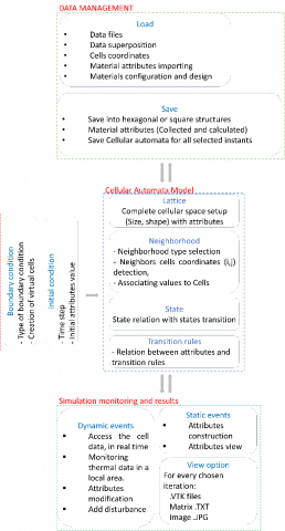
The modeling code was developed under python object-oriented programming. Figure 6 illustrates the data processing and simulation workflow.
Figure 6. Principle of cellular automata model
Data management: In data management section, each cell is linked to a vector corresponding to its attributes. To ensure compatibility with our simulation, a meticulous processing analysis is conducted to convert the data into the (.xy) structure. Subsequently, the data map is loaded, serving as the foundation for constructing a cellular lattice. This lattice is constructed with uniform pixel sizes and variable resolutions.
Initial and boundary conditions: Before initiating the simulation, we establish the initial conditions for each cell and set boundary conditions for the virtual counterparts.
Simulation monitoring: As the simulation unfolds, we monitor the evolution of each attribute over time and gather real-time information about the cells. To facilitate comprehensive visualization and analysis, the obtained results can be exported in various formats such as VTK, TXT, and JPG files. This enables a detailed examination of the simulation outcomes, supporting a deeper understanding of the dynamic processes.
4.2 Model evaluation
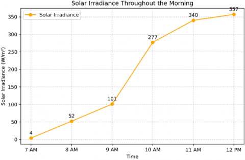
To evaluate the accuracy of our model, we conducted a comparative study by comparing the simulated temperature distribution with real infrared (IR) thermal imaging of a building facade. First, we used a LiDAR scanner to capture the facade geometry and constructed a cellular lattice with a cell size of 0.7 cm² in Figure 7. The simulation was executed with a 30-second time step, using real solar irradiance values from 7 AM to 12 PM as shown in Figure 8. We use brick, concrete on column and glass on windows area. Thermal proprieties of used materials are in Table 2. Initial temperature was estimated from metrological data at 11℃.
Figure 7. Simulation of lidar captured facade at 12 PM (t600)
Figure 8. Solar irradiance values from 7 AM to 12 PM
Table 2. Thermal properties of materials
|
Materials |
Thermal Conductivity [W/(m℃)] |
Density [Kg/m3] |
Specific Heat [J/kg.℃] |
|
Brick |
0.7 |
1500 |
800 |
|
Glass |
1.1 |
2200 |
792 |
|
Concrete |
1.33 |
2400 |
840 |
|
Steel |
45.0 |
7000 |
420 |
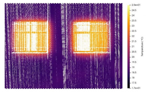
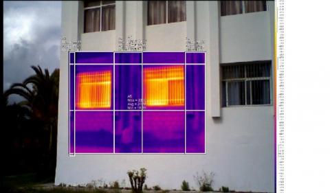
To compare simulated and real temperatures, using a Fluke Ti25 thermal imager, we captured an IR thermal image of the facade at 12 PM in Figure 9. Since windows contain metallic elements that tend to appear artificially hot (with up to 7℃ differences from glass in windows) in IR thermal imaging, we excluded them from the comparison. The presence of metals does not significantly impact the thermal behavior of the building envelope in a way relevant to this study, ignoring windows from comparison in this case ensures a more accurate validation process. We selected five distinct non-window zones, which are highlighted with white squares in Figure 9.
Figure 9. IR thermal image of the facade at 12 pm
From these five zones, we extracted mean, maximum, and minimum temperatures for validation. The extracted values for experiment and simulation are in Table 3.
Table 3. Statistical values of experimental and simulation results
|
Results |
Max Temperature (℃) |
Min Temperature (℃) |
Mean Temperature (℃) |
|
Experiment |
22.66 |
17.66 |
20.092 |
|
Simulation |
23.73 |
18.22 |
19.892 |
The maximum temperature from the IR camera (22.66℃) is slightly lower than the simulation result (23.7291℃), with a difference of around 1.07℃. The minimum temperature from the IR camera (17.66℃) is also slightly lower than the simulation value (18.2258℃), with a difference of about 0.57℃. The mean temperature from IR camera measurements (20.092℃) is close to the mean of the simulation (19.892℃), with a difference of 0.2℃.
4.3 Simulation description
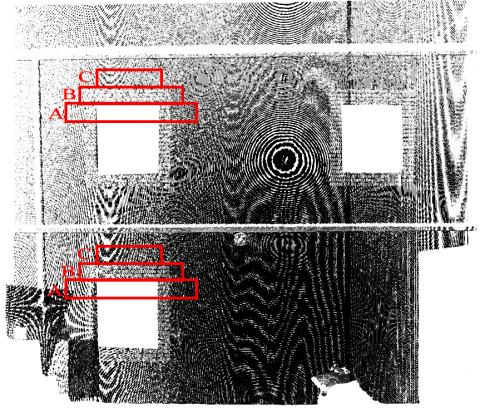
In this application, we captured the building’s geometry using a LiDAR FARO scanner. The data provided a precise 3D digital representation of the facade. We generate the CA lattice in Figure 10 using the process described in Figure 1. Our primary goal for this simulation was to analyze how external shading configurations can impact the thermal performance of the building facade.
Figure 10. Facade Lattice taken from LiDAR, after pre-processing and the implemented shading configuration
For each cell, we calculate the solar power based on the corresponding irradiance and the area of the cell. To calculate solar radiation on a surface area per cell, we use the solar radiation intensity (W/m2). In the studied region (Northern Morocco) the typical solar irradiation on a clear and sunny day is around 1000 W/m2 at noon.
Shaded cells experience significantly lower solar gains compared to unshaded ones. We incorporate the thermal impact of shading into the model by reducing the amount of direct solar irradiance in these areas, which, in turn influences the temperature and heat transfer rates of the shaded cells.
In this application, we choose shading above windows, representing a traditional Moroccan shading device. We represent this shading by using 3 solar irradiance levels, categorized into three categories A, B and C highlighted in red in Figure 10: A: 300 W/m2, B: 500 W/m2, C: 700 W/m2.
Simulation conditions are:
Layer area: Width × Height = 8 m2 × 12 m2 = 96 m2
Number of cells: 15172 cells
Cell size: 0.7 cm2
Duration: sunrise to midday: 6 Hours
Time step used: 15 seconds- Initial temperature: 20℃; Solar irradiation (unshaded cells): 1000 W/m2
Boundary condition: The boundary is considered adiabatic (no heat exchange at the boundaries cells)
The thermal proprieties of materials used are in Table 2.
4.4 Sensitivity analysis
To ensure the correct choice of cell size and time step, we have performed a sensitivity analysis to examine the impact of different spatial and temporal resolutions on simulation accuracy and computational efficiency. We set a high-resolution reference, with a cell size equal to 0.5 cm² and a fixed time step of 5 seconds, this reference was used for comparison. The results in Table 4 indicate that a cell size of 0.7 cm² provide high accuracy (Emax < 0.1) and (Emean < 1.0), increasing the cell size impact the accuracy significantly.
Table 4. Descriptive statistics of the sensitivity analysis
|
Cell Size (cm²) |
Max Temperature (℃) |
Mean Temperature (℃) |
Max Temperature Absolute Error |
Mean Temperature Absolute Error |
|
0.5 |
63.103 |
40.756 |
0 |
0 |
|
0.7 |
63.148 |
41.6184 |
0.045 |
0.8624 |
|
1.5 |
63.4694 |
44.6748 |
0.3664 |
3.9188 |
|
3.0 |
63.4554 |
45.9265 |
0.3524 |
5.1705 |
For the temporal analysis, we fixed the cell size to 0,7 cm², and we compared four-time steps sizes (5 s, 15 s, 30 s and 60 s). As shown in Table 5, a time step at 5 seconds results in a higher runtime, requiring more computational effort. As we increase the time step, the simulation runtime decreases. However, increasing the time step above 30 seconds introduces oscillations and numerical instabilities.
Table 5. Time step and simulation runtime
|
Time Step (s) |
Simulation Runtime (s) |
|
5 |
420 |
|
15 |
120 |
|
30 |
63 |
|
60 |
38 |
4.5 Results and discussion
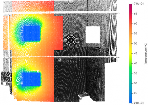
Figure 11 highlights the effect of using shading device above windows, by showing a side-to-side comparison between shaded scenario and unshaded scenario after 1440 iteration (at 12 pm). From the figure, we can see the differences in temperature distribution across the facade section around windows, between the case without shading and the case with shading. Areas with cells shaded display lower temperatures, this does not affect cells with lower irradiance levels only but areas around those cells also experience a decrease in temperature. This clearly displays the effect of solar control (shading in this case) on building facade temperature, especially in climates with high solar intensity.
(a) Without shading
(b) With shading
Figure 11. Temperature distribution across the facade section around windows during midday t1440
Using a histogram, we can see the distribution of the number of cells across temperature ranges at midday (t1440) in Figure 12. This result emphasizes further the effect of shading on the building facade. At lower temperature ranges, the number of cells is higher in the scenario with shading than in the unshaded case. Also, in the shading case, as we increase the range of temperature, we observe an increase in the number of cells, opposite to what is displayed for the unshaded case. This suggests a stabilization of temperature across the facade when shading is applied. The overall temperature not only decreased but also stabilized, which preventing temperature fluctuations caused by extreme solar exposure.
Figure 12. Number of cells for 10 temperature ranges
Descriptive statistics in Table 6, includes statistical metrics such as mean temperature Tmean and maximum temperature Tmax for each scenario, such metrics provide a quantitative measure of temperature distribution across the façade. The results indicate a mean temperature reduction of 9.90% in shaded scenario compared to unshaded scenario, demonstrating the impact of shading on heat mitigation.
Table 6. Descriptive statistics of simulations results
|
Shading Status |
Max Temperature (℃) |
Mean Temperature (℃) |
M2 |
|
No shading |
64.4639 |
54.7574 |
1.96E+06 |
|
With shading |
64.472 |
49.3348 |
1.08E+06 |
After calculating standard deviation using Eq. (13), we find the shaded scenario has a lower standard deviation of σ=8.43℃, indicating more uniform and stable temperatures, while the unshaded scenario has a higher standard deviation of σ=11.36℃, reflecting greater thermal variability. This suggests that shading significantly reduces temperature fluctuations.
$\sigma =\sqrt{\frac{M2}{N-1}}$ (13)
We quantify conduction heat gain, comparing the two scenarios, by calculating for each material conduction heat flux. Geometrical data for each material are in Table 7 and thermal proprieties of each material are in Table 2. We use mean temperature from the simulation results Table 6, and we set indoor temperature setpoint to 25℃.
For steady-state conduction, the heat transfer Q (W) is given in Eq. (14).
$Q=\frac{{kA}\Delta{T}}{d}$ (14)
Table 7. Geometrical data of materials in simulation
|
Materials |
Thickness, d (m) |
Exposed Area, A (m²) |
Difference, ΔQ (W) |
|
Brick |
0.15 |
72 |
1827 |
|
Glass |
0.02 |
12 |
3564 |
|
Concrete |
0.15 |
12 |
574 |
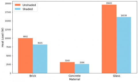
The calculated heat load throught each material for shadded scenario and unshaded scenarion is in Figure 13.
Figure 13. Heat load through materials: unshaded vs. shaded
Summing the difference of heat loads between shaded and unshaded scenarios from all materials, we find:
${\Delta{Q}_{total}}={\Delta{Q}_{brick}}+\Delta{{Q}_{glass}}+\Delta{{Q}_{concrete}}=5965~\text{W}$
For the HVAC energy savings. The electrical energy required to remove a given cooling load is calculated using Eq. (15).
$E=\frac{Q}{COP}$ (15)
In this study, we assume that the coefficient of performance (COP) is equal to 3.5. We get the required energy for cooling one hour at noon ΔEHour.
$\Delta{{E}_{Hour}}=\frac{\Delta{{Q}_{total}}}{3.5}=\frac{5965}{3.5}=1704\text{ }\!\!~\!\!\text{ Wh}$
By analyzing the results of this application, we can draw valuable insights on the impact of shading strategies on the thermal performance of building envelopes. In passive design strategies, shading can be an important element for energy efficiency, reducing temperature fluctuations and cooling down the building envelope. Also, in regions like Northern Morocco, where solar irradiation is extreme, studying the integration of shading configuration with a precise facade data captured by LiDAR can give important energy-saving insights and improve building envelopes. This tool can be used for different architectural and environmental contexts.
4.6 Broader applicability of the model
As CA models are rule-based and can incorporate localized material properties and meteorological data, the same framework could be applied to hot-arid, temperate or cold climates by adjusting attributes such as solar radiation, convection effects and thermal material properties. Integrating LiDAR analyses with CA further enhances scalability by providing a data-driven approach to defining grid structures, enabling high-resolution thermal simulations.
However, the resolution of LiDAR data has a significant impact on computational efficiency and the accuracy of results. Higher resolution analyses provide more detailed façade geometries, improving the accuracy of heat transfer simulations by capturing thermal bridges, surface roughness and material heterogeneity. However, such complex cases come with an increased computational cost, as higher lattice resolutions require more processing power and longer simulation runtimes. A trade-off needs to be made between data accuracy and model efficiency, particularly when applying this approach to large-scale urban environments.
In this paper, we considered the integration of Terrestrial LiDAR with CA modeling. This integration is used to analyze the thermal dynamics of the building envelope. We focused on the CA lattice construction using the LiDAR data as input. The Terrestrial LiDAR captures precise geometric measurements of buildings, while CA modeling provides a local description of the thermal dynamics. We applied the model to a real building in Northern Morocco. The application captures the building's facade using FARO LiDAR. After data processing, we constructed the lattice. We compared two scenarios: the first one with the facade fully exposed to solar irradiation and the second one using shading around two windows. The results show the importance of using shading devices in decreasing the temperature of the building's facade. The LiDAR coupled to CA modeling introduces a powerful methodology to analyze the thermal performance of buildings. While the LiDAR improves the model's ability to account for real-world geometric complexity, CA provides the computational efficiency needed to simulate heat transfer over time. This approach opens new possibilities to improve the accuracy of building performance simulations and to optimize the configuration and material choices for the energy efficiency of buildings.
Future work: Dynamic shading will be incorporated as a time-dependent attribute influencing local cell states. The present study considers shading as a static feature Incorporating dynamic shading into the model can be achieved through the attributes concept, where each cell is assigned a time-dependent Shading Attribute. This attribute modifies the local solar exposure of a cell based on shading device position, external environmental conditions, or user-defined control strategies.
This work was funded by the project PPR2/2016/79; OGI-Env, with MENFPESRS and CNRST, Morocco.
[1] Talib, M.M., Croock, M.S. (2024). Optimizing energy consumption in buildings: Intelligent power management through machine learning. Mathematical Modelling of Engineering Problems, 11(3): 765-772. https://doi.org/10.18280/mmep.110321
[2] Mohammadiziazi, R., Bilec, M.M. (2020). Application of machine learning for predicting building energy use at different temporal and spatial resolution under climate change in USA. Buildings, 10(8): 139. https://doi.org/10.3390/buildings10080139
[3] Kjærgaard, M.B., Arendt, K., Clausen, A., Johansen, A., et al. (2016). Demand response in commercial buildings with an assessable impact on occupant comfort. In 2016 IEEE International Conference on Smart Grid Communications (SmartGridComm), Sydney, NSW, Australia, pp. 447-452. https://doi.org/10.1109/SmartGridComm.2016.7778802
[4] Qiu, Y., Wang, H., Zhang, Q. (2021). Energy-efficient and sustainable construction technologies and simulation optimisation methods. In 2021 International Conference on E-Commerce and E-Management (ICECEM), Dalian, China, pp. 341-351. https://doi.org/10.1109/ICECEM54757.2021.00075
[5] Yamamoto, T., Ozaki, A., Kaoru, S., Taniguchi, K. (2021). Analysis method based on coupled heat transfer and CFD simulations for buildings with thermally complex building envelopes. Building and Environment, 191: 107521. https://doi.org/10.1016/j.buildenv.2020.107521
[6] Hershcovich, C., van Hout, R., Rinsky, V., Laufer, M. (2021). Thermal performance of sculptured tiles for building envelopes. Building and Environment, 197: 107809. https://doi.org/10.1016/j.buildenv.2021.107809
[7] Maury-Micolier, A., Huang, L., Jolliet, O. (2023). Coupled mass and heat transfer modelling in building envelopes to consistently assess human exposure and energy performance in indoor environments. Journal of Building Performance Simulation, 16(6): 734-748. https://doi.org/10.1080/19401493.2023.2200377
[8] Pollyea, R.M., Fairley, J.P. (2011). Estimating surface roughness of terrestrial laser scan data using orthogonal distance regression. Geology, 39(7): 623-626. https://doi.org/10.1130/G32078.1
[9] Tan, Y., Liu, X., Jin, S., Wang, Q., Wang, D., Xie, X. (2023). A terrestrial laser scanning-based method for indoor geometric quality measurement. Remote Sensing, 16(1): 59. https://doi.org/10.3390/rs16010059
[10] Shen, N., Wang, B., Ma, H., Zhao, X., Zhou, Y., Zhang, Z., Xu, J. (2023). A review of terrestrial laser scanning (TLS)-based technologies for deformation monitoring in engineering. Measurement, 223: 113684. https://doi.org/10.1016/j.measurement.2023.113684
[11] Wang, C., Cho, Y.K., Gai, M. (2013). As-is 3D thermal modeling for existing building envelopes using a hybrid LIDAR system. Journal of Computing in Civil Engineering, 27(6): 645-656. https://doi.org/10.1061/(ASCE)CP.1943-5487.0000273
[12] Borrmann, D., Nüchter, A., Đakulović, M., Maurović, I., Petrović, I., Osmanković, D., Velagić, J. (2012). The project thermalmapper–thermal 3D mapping of indoor environments for saving energy. IFAC Proceedings Volumes, 45(22): 31-38. https://doi.org/10.3182/20120905-3-HR-2030.00045
[13] Ham, Y., Golparvar-Fard, M. (2013). An automated vision-based method for rapid 3D energy performance modeling of existing buildings using thermal and digital imagery. Advanced Engineering Informatics, 27(3): 395-409. https://doi.org/10.1016/j.aei.2013.03.005
[14] Kassogué, H., Bernoussi, A., Maâtouk, M., Amharref, M. (2017). A two scale cellular automaton for flow dynamics modeling (2CAFDYM). Applied Mathematical Modelling, 43: 61-77. https://doi.org/10.1016/j.apm.2016.10.034
[15] Byari, M., Bernoussi, A., Jellouli, O., Ouardouz, M., Amharref, M. (2022). Multi-scale 3D cellular automata modeling: Application to wildland fire spread. Chaos, Solitons & Fractals, 164: 112653. https://doi.org/10.1016/j.chaos.2022.112653
[16] Kukaram, G., Ramasamy, V. (2023). A novel approach of 1D cellular automata in cryptosystem. Mathematical Modelling of Engineering Problems, 10(6): 2121-2126. https://doi.org/10.18280/mmep.100623
[17] Aziza, R., Borgi, A., Zgaya, H., Guinhouya, B. (2016). Simulating complex systems-complex system theories, their behavioural characteristics and their simulation. In 8th International Conference on Agents and Artificial Intelligence, Rome, Italy. https://doi.org/10.5220/0005684602980305
[18] Bobkov, S., Galiaskarov, E., Astrakhantseva, I. (2021). The use of cellular automata systems for simulation of transfer processes in a non-uniform area. In CEUR Workshop Proceedings, 2843.
[19] Saiz, A., Urchueguía, J. F., Martos, J. (2010). A cellular automaton based model simulating HVAC fluid and heat transport in a building. Modeling approach and comparison with experimental results. Energy and Buildings, 42(9): 1536-1542. https://doi.org/10.1016/j.enbuild.2010.03.024
[20] Khaddor, Y., samed Bernoussi, A., Amharref, M., Ouardouz, M. (2024). Thermal performance of buildings using phase change materials: Cellular automata modeling. In ICHMT Digital Library Online. https://doi.org/10.1615/ICHMT.2024.CHT-24
[21] Wąs, J., Karp, A., Łukasik, S., Pałka, D. (2020). Modeling of fire spread including different heat transfer mechanisms using cellular automata. In Computational Science–ICCS 2020: 20th International Conference, Amsterdam, The Netherlands, pp. 445-458. https://doi.org/10.1007/978-3-030-50371-0_33
[22] Wolfram, S. (1984). Universality and complexity in cellular automata. Physica D: Nonlinear Phenomena, 10(1-2): 1-35. https://doi.org/10.1016/0167-2789(84)90245-8
[23] Burzyński, M., Cudny, W., Kosiński, W. (2004). Cellular automata: Structures and some applications. Journal of Theoretical and Applied Mechanics, 42(3): 461-482.
[24] Yamamoto, T. (1996). Self-organization between local and non-local interaction in 2D cellular automata. In Proceedings of IEEE International Conference on Evolutionary Computation, Nagoya, Japan, pp. 300-305. https://doi.org/10.1109/ICEC.1996.542379
[25] Byari, M., Bernoussi, A., Ouardouz, M., Amharref, M. (2022). Protector control of 3D cellular automata via space attributes: Application to wildland fire. Journal of Cellular Automata, 16: 381-399.
[26] Kong, D., Yang, Y., Sa, X., Wei, X., et al. (2023). Evaluation of the impact of input-data resolution on building-energy simulation accuracy and computational load—A case study of a low-rise office building. Buildings, 13(4): 861. https://doi.org/10.3390/buildings13040861