Sabah Ali Rahi*![]() | Raid Kamel Naji
| Raid Kamel Naji![]()
© 2024 The authors. This article is published by IIETA and is licensed under the CC BY 4.0 license (http://creativecommons.org/licenses/by/4.0/).
OPEN ACCESS
A mathematical model has been created and investigated that simulates the relationship between predator and prey with the appearance of an infectious disease in the predator population and additional food reservoirs for the predator. The prey declines its rate of growth due to it is enforced by the predator's rage to seek out a place where it will feel scared and safe. The bounds, existence, and uniqueness of the solution of the suggested model are examined. The local stability of the model at feasible equilibrium points was calculated. The Lyapunov function is utilized to identify the basin of attraction for each equilibrium point. The possibility of bifurcation when the parameters vary is also carefully discussed. Numerical simulations were then used to validate the analytical conclusions and provide insight into how parameter changes impacted the model's dynamics. Different attractors of the system are obtained, such as point, periodic, and nonlinear centers.
fear, refuge, disease, stability, bifurcation
Ecology and epidemiology are distinct disciplines that encompass significant areas of research. However, it is worth noting that these systems have certain correlations, and exploring their integration might reveal significant patterns. Eco-epidemiology is an emerging field within the realm of mathematical biology that simultaneously integrates ecological and epidemiological factors. The eco-epidemiological method covers the investigation of transmissible diseases within ecological systems, specifically focusing on the community and population levels. The methodical analytical approach that applies demographic, sociological, and biological viewpoints to the study of health-related problems is called eco-epidemiology [1-4].
Despite being a relatively new topic of research, eco-epidemiology is quickly gaining popularity as the connectivity of ecological and epidemiological systems is understood more and more. For instance, factors like habitat loss, climate change, and a drop in biodiversity may have an impact on the transmission of infectious illnesses. However, the existence of infectious diseases can have an impact on the dynamics of ecological systems. The intricate relationships between ecological and epidemiological systems can be studied using eco-epidemiological models. These models can help us comprehend how ecological factors influence the spread of illnesses and how the presence of infectious diseases affects ecological systems. This data may be used to support conservation and public health policies. The eco-epidemiological prey-predator model that Anderson and May [1, 2] pioneered was used to study the persistence, invasion, and transmission of illnesses. Numerous eco-epidemiological scholars have since Anderson and May’s work studied ecological systems with the disease in either prey [5-11] or a predator [12-17] or in both populations [18-21], and all cited literature therein. According to Ashwin et al. [11] investigation of the prey-predator model, diseased prey can cause susceptible prey to become fearful, and the predator can eat its prey through Holling-type interactions. It is suggested to use an eco-epidemiological system that includes a disease that is spread both vertically and horizontally among predatory organisms [17]. It is presumed that the predator is experiencing the impacts of nonlinear type harvesting. Finally, Bezabih et al. [21] built a prey-predator model with five compartments and treated both the prey and the predator who were infected. They used type II functional response and basic kinetic mass action functions to express the rates of incidence of predation and the transmission of illness respectively.
Conversely, the predator-prey relationship is one of many interspecies interactions that are crucial in influencing the complicated biological systems' dynamics seen on this diversified planet. According to research, its significance goes beyond interactions between predator and prey species because it greatly affects the ecosystem's overall structure [22]. According to conventional wisdom, prey species incur growth costs because predators grow by eating their prey. Since predation has historically been seen as the essential component in interactions between predators and their prey, many studies on predator-prey systems have been undertaken recently under the assumption that predation is the main way of contact among predators and their prey [23-28]. However, numerous new empirical and theoretical research has cast doubt on the classical perspective. Studies have shown how indirect factors, like fear, make a big difference to the dynamics between predators and prey as well as the ecosystem as a whole. The concept of fear was initially formulated mathematically by Wang et al. [29]. Prey individuals have been seen to experience psychological stress from predator species, which causes changes in their typical foraging activity. The worry of being trapped and killed by predators is said to be the cause of this tension. This improves the prey species' chances of surviving in the short term, which benefits them in certain ways, but it may be highly damaging in the long run. Furthermore, apart from their dietary preferences, the perceived threat from predators reduces their reproductive rate and chances of survival relative to average adults. Several recent field tests and theoretical analyses support these claims. Paradoxical results have been found in several studies, including the possibility that the indirect effects of fear could outweigh the direct consequences of predatory behavior [10, 30-32], and others. Fear, predator-dependent refuge, and quadratic fixed effort harvesting were defined and studied by Jamil and Naji [33] using a modified Leslie-Gower prey-predator model, with the help of the Beddington-DeAngelis type of functional response. By altering the abundance of the predator population, Nadim et al. [34] investigated the possible applications of fear in prey as a result of error-based Z-control methods and signals of predators. However, Abbas and Naji [35] built and investigated an ecological food web system with two predators battling for prey while exhibiting fear.
Prey refuge, which offers a place for prey to hide, is also the most important component that greatly affects the dynamic behavior of prey-predator systems. Animal refuges might be physical habitats like caverns, thickets, or burrows, or they can be behavioral adaptations like camouflage or concealment, which protect animals from predators. Refuges have the potential to reduce predation rates and contribute to the stabilization of populations of prey, but they can also have unintended consequences on the population of predators, such as making them spend more time looking for prey [36]. Prey species' use of refuges is a complicated behavior that is influenced by several variables, including the refuge's characteristics, the perceived threat of predation, and the related costs of seeking refuge. For instance, prey may be less likely to use a refuge if it is shoddily built or challenging to reach. According to Smith [37], in prey-predator models, the benefit of refuge exploited by prey is typically accounted for by a constant proportion or a constant number of the prey population that is protected from predation. Prey refuge has been studied in many mathematical models of prey-predator dynamics, see for example [38-40] for constant number refuge and [41-49] for constant proportional of prey. The models outlined above have shown that the existence of a prey refuge can have a major impact on the dynamics and stability of these systems. For instance, several models have shown how prey refuges can lower the probability of the extinction of prey populations. In contrast, recently several models have been proposed and studied where the presence of a refuge for prey is influenced by the populations of prey and predator simultaneously and shown that prey refuge may cause both populations of prey and predators to experience periodic oscillations [33, 50-54].
Due to the importance of the prey and predator systems in environmental and economic terms for humans as well as the high incidence of infectious illnesses resulting from the mixing and interaction of these organisms with one another, in contrast to previous studies, the purpose of this paper is to suggest and study a new eco-epidemiological model that combines all the above three stated biological factors (such as infectious disease, fear, and predator-dependent refuge), which are mostly present in the real-world ecological systems together. Based on our basic knowledge, none of the existing mathematical models have incorporated these biological factors, despite their presence in the real world.
This section presents a mathematical formulation of the prey-predator system that includes infectious disease in predators. Since prey and Predator do not exist alone in the environment, but rather exist within a large interacting group of organisms, so we assumed it is presumed that there is a second supply of food for predators. The intensity of predation sends victims into a panic, which prompts them to look for a haven that corresponds with the density of predators to protect themselves. The presence of the disease also weakens the predator's strength and speed, so the illness inhibits the infected predators from being linked with the predation process due to the weakness of the infected predator and is spread by contact between the healthy predator and the infected predator. Therefore, following these assumptions, the following set of nonlinear ODEs simulates the dynamics of an eco-epidemiological system.
$\begin{aligned} & \frac{d X}{d T}=\frac{r X}{1+n Y}-a X^2-\frac{b(1-m Y) X Y}{c+u v A+(1-m Y) X}, \\ & \frac{d Y}{d T}=\frac{e b((1-m Y) X+v A) Y}{c+u v A+(1-m Y) X}-k Y Z-d_1 Y, \\ & \frac{d Z}{d T}=k Y Z-d_2 Z,\end{aligned}$ (1)
where, X(T), Y(T), and Z(T) are the densities at time T for the prey, susceptible predator, and infected predator respectively with nonnegative initial conditions X(0)≥0, Y(0)≥0 and Z(0)≥0. While the parameters can be described in Nomenclature section.
Considering the dimensionless parameters and variables listed below:
$\begin{gathered}t=r T, x=\frac{a}{r} X, y=\frac{a b}{r^2} Y, z=\frac{k}{r} Z, \\ \delta_1=\frac{n r^2}{a b}, \delta_2=\frac{m r^2}{a b}, \delta_3=\frac{a c}{r}, \delta_4=\frac{a u v A}{r}, \delta_5=\frac{e b}{r}, \\ \delta_6=\frac{a v A}{r}, \delta_7=\frac{d_1}{r}, \delta_8=\frac{k r}{a b}, \delta_9=\frac{d_2}{r} .\end{gathered}$ (2)
System (1) becomes in the following dimensionless form:
$\begin{aligned} & \frac{d x}{d t}=x\left[\frac{1}{1+\delta_1 y}-x-\frac{\left(1-\delta_2 y\right) y}{\delta_3+\delta_4+\left(1-\delta_2 y\right) x}\right]=x h_1(x, y, z), \\ & \frac{d y}{d t}=y\left[\frac{\delta_5\left[\left(1-\delta_2 y\right) x+\delta_6\right.}{\delta_3+\delta_4+\left(1-\delta_2 y\right) x}-z-\delta_7\right]=y h_2(x, y, z), \\ & \frac{d z}{d t}=z\left[\delta_8 y-\delta_9\right]=z h_3(x, y, z),\end{aligned}$ (3)
with x(0)≥0, y(0)≥0, and z(0)≥0.
Theorem 1. The solutions of the system are uniformly limited within a sub-region of its domain, under the following sufficient condition.
$\frac{\delta_5 \delta_6}{\delta_3+\delta_4}<\delta_7$ (4)
where, $\varepsilon=\min \left\{1, \delta_7-\frac{\delta_5 \delta_6}{\delta_3+\delta_4}, \delta_9\right\}$.
Proof. From the equations of the system, we have:
$\frac{d x}{d t} \leq x\left[\frac{1}{1+\delta_1 y}-x\right] \leq x(1-x)$.
Therefore, it is easy to check that x(t)≤1 for t→∞.
Now, define U(t)=x(t)+y(t)+z(t), then by using the biological facts that 0<δ5<1, 0<δ8<1, with condition (4) it is obtained that:
$\frac{d U}{d t} \leq 2 x-x-\left(\delta_7-\frac{\delta_5 \delta_6}{\delta_3+\delta_4}\right) y-\delta_9 z \leq 2-\varepsilon U$,
Now, by solving the above differential inequality using the initial value $U(0)=U_0$, it is found that:
$U(t) \leq \frac{2}{\varepsilon}+\left(U_0-\frac{2}{\varepsilon}\right) e^{-\varepsilon t}$, and then $\lim _{t \rightarrow \infty} U(t) \leq \frac{2}{\varepsilon}$.
Hence, all the system (3) solutions in the region $\Omega=\left\{(x, y, z) \in \mathbb{R}^3: 0<x \leq 1, x+y+z<\frac{2}{\varepsilon}\right\}$ are uniformly limited.
Direct computation shows that system (3) has at most six non-negative equilibrium points, which can be described as follows:
The vanishing equilibrium point (VEP) E0=(0,0,0) and the first axial equilibrium point (FAEP) E1=(1,0,0) always exist. While the second axial equilibrium point (SAEP) $E_2=(0, \bar{y}, 0)$, where $\bar{y}>0$ exists if and only if the condition listed below is met:
$\frac{\delta_5 \delta_6}{\delta_3+\delta_4}=\delta_7$ (5)
The disease-free equilibrium point (DFEP) $E_3=(\hat{x}, \hat{y}, 0)$, where $\hat{x}=\frac{-\delta_5 \delta_6+\delta_3 \delta_7+\delta_4 \delta_7}{\left(1-\delta_2 y\right)\left(\delta_5-\delta_7\right)}$, and $\hat{y}$ is a positive root of the following polynomial equation.
$N_4 y^4+N_3 y^3+N_2 y^2+N_1 y+N_0=0$ (6)
with:
$\begin{aligned} & N_4=\delta_1 \delta_2^2 \delta_5^2-2 \delta_1 \delta_2^2 \delta_5 \delta_7+\delta_1 \delta_2^2 \delta_7^2, \\ & N_3=-2 \delta_1 \delta_2 \delta_5^2+\delta_2^2 \delta_5^2+4 \delta_1 \delta_2 \delta_5 \delta_7-2 \delta_2^2 \delta_5 \delta_7 -2 \delta_1 \delta_2 \delta_7^2+\delta_2^2 \delta_7^2 \\ & N_2=\delta_1 \delta_5^2-2 \delta_2 \delta_5^2-2 \delta_1 \delta_5 \delta_7+4 \delta_2 \delta_5 \delta_7 +\delta_1 \delta_7^2-2 \delta_2 \delta_7^2 \\ & N_1=\delta_5^2+\delta_2 \delta_3 \delta_5^2+\delta_2 \delta_4 \delta_5^2-\delta_2 \delta_5^2 \delta_6-\delta_1 \delta_3 \delta_5^2 \delta_6 \\ & -\delta_1 \delta_4 \delta_5^2 \delta_6+\delta_1 \delta_5^2 \delta_6^2-2 \delta_5 \delta_7-\delta_2 \delta_3 \delta_5 \delta_7 \\ & +\delta_1 \delta_3^2 \delta_5 \delta_7-\delta_2 \delta_4 \delta_5 \delta_7+2 \delta_1 \delta_3 \delta_4 \delta_5 \delta_7 \\ & +\delta_1 \delta_4^2 \delta_5 \delta_7+\delta_2 \delta_5 \delta_6 \delta_7-\delta_1 \delta_3 \delta_5 \delta_6 \delta_7 \\ & -\delta_1 \delta_4 \delta_5 \delta_6 \delta_7+\delta_7^2 \\ & N_0=-\delta_3 \delta_5^2-\delta_4 \delta_5^2+\delta_5^2 \delta_6-\delta_3 \delta_5^2 \delta_6-\delta_4 \delta_5^2 \delta_6 \\ & +\delta_5^2 \delta_6^2+\delta_3 \delta_5 \delta_7+\delta_3^2 \delta_5 \delta_7+\delta_4 \delta_5 \delta_7+2 \delta_3 \delta_4 \delta_5 \delta_7 \\ & +\delta_4^2 \delta_5 \delta_7-\delta_5 \delta_6 \delta_7-\delta_3 \delta_5 \delta_6 \delta_7-\delta_4 \delta_5 \delta_6 \delta_7 \\ & \end{aligned}$
The disease-free point exists uniquely in the xy-plane if and only if the conditions listed below are met:
$\left.\begin{array}{c}\frac{\delta_5 \delta_6}{\delta_3+\delta_4}<\delta_7<\delta_5 \\ \text { or } \\ \delta_5<\delta_7<\frac{\delta_5 \delta_6}{\delta_3+\delta_4}\end{array}\right\}$ (7)
with one of the following conditions:
$\left.\begin{array}{l}N_4>0, N_3>0, N_2 \neq 0, N_1<0, N_0<0 \\ N_4<0, N_3<0, N \neq 0, N_1>0, N_0>0 \\ N_4>0, N_3>0, N_2>0, N_1>0, N_0<0 \\ N_4>0, N_3<0, N_2<0, N_1<0, N_0<0 \\ N_4<0, N_3<0, N_2<0, N_1<0, N_0>0 \\ N_4<0, N_3>0, N_2>0, N_1>0, N_0>0\end{array}\right\}$ (8)
The prey-free equilibrium point (PFEP) $E_4=(0, \breve{y}, \check{z})$, where $\breve{y}=\frac{\delta_9}{\delta_8}$, and $\check{z}=\frac{\delta_5 \delta_6-\delta_3 \delta_7-\delta_4 \delta_7}{\delta_3+\delta_4}$ which exists in the interior of the first quadrant of the yz-plane if and only if.
$\delta_7<\frac{\delta_5 \delta_6}{\left(\delta_3+\delta_4\right)}$ (9)
Finally, the co-existing equilibrium point (CEEP) E5=(x*, y*, z*), can be determined by solving the following system.
$\left.\begin{array}{l}h_1(x, y, z)=0 \\ h_2(x, y, z)=0 \\ h_3(x, y, z)=0\end{array}\right\}$ (10)
Direct computation shows that:
$y^*=\frac{\delta_9}{\delta_8}, z^*=\frac{\delta_5\left(\delta_6+\left(1-\frac{\delta_2 \delta_9}{\delta_8}\right) x^*\right)}{\delta_3+\delta_4+\left(1-\frac{\delta_2 \delta_9}{\delta_8}\right) x^*}-\delta_7$ (11)
while z* is a positive root of the equation:
$\begin{gathered}-\left(1-\frac{\delta_2 \delta_9}{\delta_8}\right)\left(1+\frac{\delta_1 \delta_9}{\delta_8}\right) x^2 \\ +\left(\left(1-\frac{\delta_2 \delta_9}{\delta_8}\right)-\left(\delta_3+\delta_4\right)\left(1+\frac{\delta_1 \delta_9}{\delta_8}\right)\right) x \\ +\delta_3+\delta_4-\frac{\delta_9}{\delta_8}\left(1-\frac{\delta_2 \delta_9}{\delta_8}\right)\left(1+\frac{\delta_1 \delta_9}{\delta_8}\right)=0\end{gathered}$ (12)
Clearly, the co-existing point exists uniquely in the interior of $\mathbb{R}_{+}^3$ if and only if the following requirements listed below are met.
$\delta_7<\frac{\delta_5\left(\delta_6+\left(1-\frac{\delta_2 \delta_9}{\delta_8}\right) x^*\right)}{\delta_3+\delta_4+\left(1-\frac{\delta_2 \delta_9}{\delta_8}\right) x^*}$ (13)
$0<\frac{\delta_9}{\delta_8}\left(1-\frac{\delta_2 \delta_9}{\delta_8}\right)\left(1+\frac{\delta_1 \delta_9}{\delta_8}\right)<\delta_3+\delta_4$ (14)
A linear stability analysis of the system (3) is implemented to examine its local behavior near the equilibrium points. Using this technique, the model equations are linearized near an equilibrium point, and the Jacobian matrix's eigenvalues (EVEs) are determined. The sign of the real parts of the EVEs specifies the stability of the system. The equilibrium is stable if every eigenvalue (EVE) has a negative real part; and unstable if any EVE has a positive real part. Now, the variational matrix (VM) at the point (x, y, z) is determined by:
$\mathcal{V}=\left[a_{i j}\right]_{3 \times 3}$ (15)
where,
$\begin{aligned} a_{11}= & -x+\frac{1}{1+\delta_1 y}-\frac{y\left(1-\delta_2 y\right)}{x\left(1-\delta_2 y\right)+\delta_3+\delta_4} + x\left(-1+\frac{y\left(1-\delta_2 y\right)^2}{\left(x\left(1-\delta_2 y\right)+\delta_3+\delta_4\right)^2}\right). \\ a_{12}= & x\left(-\frac{\delta_1}{\left(1+\delta_1 y\right)^2}-\frac{x y \delta_2\left(1-\delta_2 y\right)}{\left(x\left(1-\delta_2 y\right)+\delta_3+\delta_4\right)^2}\right. +\frac{\delta_2 y}{x\left(1-\delta_2 y\right)+\delta_3+\delta_4} \left.-\frac{1-\delta_2 y}{x\left(1-\delta_2 y\right)+\delta_3+\delta_4}\right). \\ a_{13}= & 0 . \quad \\ a_{21}= & y\left(\frac{\left(1-\delta_2 y\right) \delta_5}{x\left(1-\delta_2 y\right)+\delta_3+\delta_4}-\frac{\left(1-\delta_2 y\right) \delta_5\left(x\left(1-\delta_2 y\right)+\delta_6\right)}{\left(x\left(1-\delta_2 y\right)+\delta_3+\delta_4\right)^2}\right) . \\ a_{22}= & \frac{\delta_5\left(x\left(1-\delta_2 y\right)+\delta_6\right)}{x\left(1-\delta_2 y\right)+\delta_3+\delta_4}-\frac{\delta_2 \delta_5 x y}{x\left(1-\delta_2 y\right)+\delta_3+\delta_4} + \frac{x \delta_2 \delta_5\left(x\left(1-\delta_2 y\right)+\delta_6\right)}{\left(x\left(1-\delta_2 y\right)+\delta_3+\delta_4\right)^2} y-\delta_7-z. \\ a_{23}= & -y . \\ a_{31}= & 0 . \\ a_{32}= & \delta_8 z . \\ a_{33}= & \delta_8 y-\delta_9 .\end{aligned}$
Consequently, the (VM) at the VEP becomes:
$\mathcal{V}\left(E_0\right)=\left[\begin{array}{ccc}1 & 0 & 0 \\ 0 & \frac{\delta_5 \delta_6}{\delta_3+\delta_4}-\delta_7 & 0 \\ 0 & 0 & -\delta_9\end{array}\right]$ (16)
Obviously, $\mathcal{V}\left(E_0\right)$ has the following EVEs μ10=1, $\mu_{20}=\frac{\delta_5 \delta_6}{\delta_3+\delta_4}-\delta_7$, and μ30=-δ9. Then the point E0 is a saddle point.
The VM at the FAEP becomes:
$\mathcal{V}\left(E_1\right)=\left[\begin{array}{ccc}-1 & -\delta_1-\frac{1}{1+\delta_3+\delta_4} & 0 \\ 0 & \frac{\delta_5\left(1+\delta_6\right)}{1+\delta_3+\delta_4}-\delta_7 & 0 \\ 0 & 0 & -\delta_9\end{array}\right]$ (17)
Obviously, $\mathcal{V}\left(E_1\right)$ has the following EVEs μ11=-1, $\mu_{21}=\frac{\delta_5\left(1+\delta_6\right)}{1+\delta_3+\delta_4}-\delta_7$, and μ31=-δ9. Then the point E1 is a stable node or a saddle point if and only if the conditions listed below are met respectively. It is a non-hyperbolic point otherwise.
$\frac{\delta_5\left(1+\delta_6\right)}{1+\delta_3+\delta_4}<\delta_7$ (18)
$\delta_7<\frac{\delta_5\left(1+\delta_6\right)}{1+\delta_3+\delta_4}$ (19)
The (VM) at the SAEP E2 becomes:
$\begin{gathered}\mathcal{V}\left(E_2\right)= {\left[\begin{array}{ccc}\frac{1}{1+\delta_1 \bar{y}}-\frac{\bar{y}\left(1-\delta_2 \bar{y}\right)}{\delta_3+\delta_4} & 0 & 0 \\ \bar{y}\left(\frac{\left(1-\delta_2 \bar{y}\right) \delta_5}{\delta_3+\delta_4}-\frac{\left(1-\delta_2 \bar{y}\right) \delta_5 \delta_6}{\left(\delta_3+\delta_4\right)^2}\right) & 0 & -\bar{y} \\ 0 & 0 & \delta_8 \bar{y}-\delta_9\end{array}\right]}\end{gathered}$ (20)
Obviously, $\mathcal{V}\left(E_2\right)$ has the following EVEs $\mu_{12}=\frac{1}{1+\delta_1 \bar{y}}-\frac{\bar{y}\left(1-\delta_2 \bar{y}\right)}{\delta_3+\delta_4}$, μ22=0, and $\mu_{32}=\delta_8 \bar{y}-\delta_9$. Then the point E2 is non-hyperbolic.
The (VM) at the DFEP becomes:
$\mathcal{V}\left(E_3\right)=\left[b_{i j}\right]_{3 \times 3}$ (21)
where,
$\begin{aligned} b_{11}= & \hat{x}\left(-1+\frac{\hat{y}\left(1-\delta_2 \hat{y}\right)^2}{\left(\hat{x}\left(1-\delta_2 \hat{y}\right)+\delta_3+\delta_4\right)^2}\right) . \\ b_{12}= & -\hat{x}\left(\frac{\delta_1}{\left(1+\delta_1 \hat{y}\right)^2}+\frac{\hat{x} \hat{y} \delta_2\left(1+\delta_1 \hat{y}\right)}{\left(\hat{x}\left(1+\delta_1 \hat{y}\right)+\delta_3+\delta_4\right)^2} \right. \left.\quad+\frac{1-2 \delta_2 \hat{y}}{\hat{x}\left(1+\delta_1 \hat{y}\right)+\delta_3+\delta_4}\right). \\ b_{13}= & 0 . \\ b_{21}= & \frac{\left(\delta_3+\delta_4-\delta_6\right)\left(1-\delta_2 \hat{y}\right) \delta_5 \hat{y}}{\left(\hat{x}\left(1-\delta_2 \hat{y}\right)+\delta_3+\delta_4\right)^2} . \\ b_{22}= & \frac{\left(\delta_6-\delta_3-\delta_4\right) \delta_2 \delta_5 \hat{x} \hat{y}}{\left(\hat{x}\left(1-\delta_2 \hat{y}\right)+\delta_3+\delta_4\right)^2} . \\ b_{23}= & -\hat{y}, b_{31}=b_{32}=0, b_{33}=\delta_8 \hat{y}-\delta_9 .\end{aligned}$
Obviously, $\mathcal{V}\left(E_3\right)$ has the following characteristic equation:
$\left[\mu^2-T r_1 \mu+D e_1\right]\left[\delta_8 \hat{y}-\delta_9-\mu\right]=0$ (22)
where, $Tr_1=\hat{x}\left(-1+\frac{\hat{y}\left(1-\delta_2 \hat{y}\right)^2}{\left(\hat{x}\left(1-\delta_2 \hat{y}\right)+\delta_3+\delta_4\right)^2}\right)+\frac{\left(\delta_6-\delta_3-\delta_4\right) \delta_2 \delta_5 \hat{x} \hat{y}}{\left(\hat{x}\left(1-\delta_2 \hat{y}\right)+\delta_3+\delta_4\right)^2}$. $D e_1=b_{11} b_{22}-b_{12} b_{21}$.
Direct computation shows that Tr1<0 and De1>0 if and only if the conditions listed below are met:
$\left.\begin{array}{c}\frac{\hat{y}\left(1-\delta_2 \hat{y}\right)^2}{\left(\hat{x}\left(1-\delta_2 \hat{y}\right)+\delta_3+\delta_4\right)^2}<1 \\ \delta_6<\delta_3+\delta_4 \\ 2 \delta_2 \hat{y}<1\end{array}\right\}$ (23)
Therefore, the quadratic term of Eq. (22) has roots with negative real parts due to Routh–Hurwitz criterion. However, the last term of Eq. (22) gives the third EVE $\mu_{33}=\delta_8 \hat{y}-\delta_9$ of $\mathcal{V}\left(E_3\right)$, which is negative under the following condition:
$\delta_8 \hat{y}<\delta_9$ (24)
Hence the DFEP is a sink provided that conditions (23)-(24) hold.
The (VM) at PFEP becomes:
$\mathcal{V}\left(E_4\right)=\left[\begin{array}{ccc}\frac{1}{1+\delta_1 \check{y}}-\frac{\check{y}\left(1-\delta_2 \check{y}\right)}{\delta_3+\delta_4} & 0 & 0 \\ \frac{\left(\delta_3+\delta_4-\delta_6\right)\left(1-\delta_2 \check{y}\right) \delta_5 \check{y}}{\left(\delta_3+\delta_4\right)^2} & 0 & -\check{y} \\ 0 & \delta_8 \check{z} & 0\end{array}\right]$ (25)
Obviously, $\mathcal{V}\left(E_4\right)$ has the following EVEs:
$\mu_{14}=\frac{1}{1+\delta_1 \check{y}}-\frac{\check{y}\left(1-\delta_2 \check{y}\right)}{\delta_3+\delta_4}, \mu_{24}, \mu_{34}= \pm i \sqrt{\delta_8 \check{y} \check{z}}$ (26)
Then the point E4 is non-hyperbolic. It becomes a linear center provided that
$\frac{1}{1+\delta_1 \check{y}}<\frac{\check{y}\left(1-\delta_2 \check{y}\right)}{\delta_3+\delta_4}$ (27)
Finally, the VM at the CEEP becomes:
$\mathcal{V}\left(E_5\right)=\left[c_{i j}\right]_{3 \times 3}$ (28)
where,
$\begin{aligned} c_{11}= & x^*\left(-1+\frac{y^*\left(1-\delta_2 y^*\right)^2}{\left(\delta_3+\delta_4+x^*\left(1-\delta_2 y^*\right)\right)^2}\right) . \\ c_{12}= & -x^*\left(\frac{\delta_1}{\left(1+\delta_1 y^*\right)^2}+\frac{\delta_2 x^* y^*\left(1-\delta_2 y^*\right)}{\left(\delta_3+\delta_4+x^*\left(1-\delta_2 y^*\right)\right)^2} \right. \left.+\frac{1-2 \delta_2 y^*}{\delta_3+\delta_4+x^*\left(1-\delta_2 y^*\right)}\right). \\ c_{13}= & 0. \\ c_{21}= & \frac{\left(\delta_3+\delta_4-\delta_6\right) \delta_5\left(1-\delta_2 y^*\right) y^*}{\left(\delta_3+\delta_4+x^*\left(1-\delta_2 y^*\right)\right)^2} . \\ c_{22}= & \frac{\left(\delta_6-\delta_3-\delta_4\right) \delta_2 \delta_5 x^* y^*}{\left(\delta_3+\delta_4+x^*\left(1-\delta_2 y^*\right)\right)^2} . \\ c_{23}= & -y^*, c_{31}=c_{33}=0, c_{32}=\delta_8 z^* .\end{aligned}$
Obviously, $\mathcal{V}\left(E_5\right)$ has the following characteristic equation:
$\mu^3+C_1 \mu^2+C_2 \mu+C_3=0$ (29)
where,
$\begin{aligned} & \overline{C_1}=-\left(c_{11}+c_{22}\right), \\ & C_2=c_{11} c_{22}-c_{12} c_{21}-c_{23} c_{32}, \\ & C_3=c_{11} c_{23} c_{32}, \text { with, } \\ & \Delta=C_1 C_2-C_3=-\left(c_{11}+c_{22}\right)\left[c_{11} c_{22}-c_{12} c_{21}\right]+c_{22} c_{23} c_{32}\end{aligned}$.
Direct computation shows that C1>0, C3>0, and ∆>0 if and only if the conditions listed below are met:
$\left.\begin{array}{c}\frac{y^*\left(1-\delta_2 y^*\right)^2}{\left[x^*\left(1-\delta_2 y^*\right)+\delta_3+\delta_4\right]^2}<1 \\ \delta_6<\delta_3+\delta_4 \\ 2 \delta_2 y^*<1\end{array}\right\}$ (30)
Therefore, Eq. (29) has roots with negative real parts due to the Routh–Hurwitz criterion. Hence the CEEP E5=(x*, y*, z*) is a sink provided that conditions (30) hold.
The portion of the phase space where the iterations are specified is referred to as the basin of attraction (BoA), and any starting point within that zone will asymptotically move forward into the attractor. Moreover, the attractor will be globally asymptotically stable (G.A.S.) when the BoA equals its complete domain [55].
Theorem 2. The FAEP E1=(1,0,0) of the system (3) is a G.A.S. provided that:
$\delta_5\left(\delta_1+\frac{1}{\delta_3+\delta_4}+\frac{\delta_6}{\delta_3+\delta_4}\right)<\delta_7$ (31)
Proof: Define the following Lyapunov function:
$L_1(x, y, z)=\delta_5[x-1-\ln x]+y+\frac{1}{\delta_8} z$.
Calculate L1's derivative with regard to time, followed by certain algebraic operations, to produce:
$\begin{gathered}\frac{d L_1}{d t}=\delta_5 \frac{(x-1)}{x} \frac{d x}{d t}+\frac{d y}{d t}+\frac{1}{\delta_8} \frac{d z}{d t} \\ \leq-\delta_5 \frac{(x-1)^2}{1+\delta_1 y}-\frac{\delta_9}{\delta_8} z \\ -\left[\delta_7-\delta_5\left(\delta_1+\frac{1}{\delta_3+\delta_4}+\frac{\delta_6}{\delta_3+\delta_4}\right)\right] y\end{gathered}$
Under the condition (31) it is evident that $\frac{d L_1}{d t}$ is negative definite. Hence E1 is G.A.S. on $\mathrm{R}_{+}^3$, and the proof is complete.
Theorem 3. The SAEP $E_2=(0, \bar{y}, 0)$ of the system (3) has a BoA $B\left(E_2\right)=\left\{(x, y, z) \in \mathrm{R}_{+}^3: x>1, y>0, z \geq 0\right\}$ if:
$\bar{y}<\frac{\delta_9}{\delta_8}$ (32)
Proof: Consider the following function:
$L_2(x, y, z)=\delta_5 x+\left[y-\bar{y}-\bar{y} \ln \frac{y}{\bar{y}}\right]+\frac{1}{\delta_8} z$.
Now, calculate L2's derivative concerning time, followed by certain algebraic operations, to produce:
$\frac{d L_2}{d t} \leq-\delta_5 \frac{x(x-1)}{1+\delta_1 y}-\left(\frac{\delta_9}{\delta_8}-\bar{y}\right) z$.
Note that, $\frac{d L_2}{d t}$ is negative semi-definite under the conditions (32) and the condition (5). Hence by using LaSalle's invariance principle, the set $S=\left\{(x, y, z) \in \mathrm{R}_{+}^3: \frac{d L_2}{d t}(x, y, z)=0\right\}$ contains only the invariant set {E1} and the function L2 is readily unbounded. Therefore, E2 is G.A.S. within the set B(E2), and the proof is complete.
Theorem 4. The DFEP $E_3=(\hat{x}, \hat{y}, 0)$ of the system (3) has a BoA given by $B\left(E_3\right)=\left\{(x, y, z) \in \mathrm{R}_{+}^3: x>\frac{\hat{x}}{\hat{Q}}\left[\delta_6+\left(1-\delta_2 \hat{y}\right) \hat{y}\right], y>0, z \geq 0\right\}$ if:
$\left.\begin{array}{l}\frac{\left(1-\delta_2 \hat{y}\right) \hat{y}}{\left(\delta_3+\delta_4\right) \hat{Q}}<1 \\ \rho_{12} \leq 2 \sqrt{\rho_{11} \rho_{22}} \\ \hat{y}<\delta_9\end{array}\right\}$ (33)
where,
$\begin{aligned} & \rho_{11}=1-\frac{\left(1-\delta_2 y\right)\left(1-\delta_2 \hat{y}\right) \hat{y}}{Q \hat{Q}}, \\ & \rho_{22}=\frac{\delta_2 \delta_5}{Q}\left[x-\frac{\hat{x}}{\hat{Q}}\left(\delta_6+\left(1-\delta_2 \hat{y}\right) \hat{y}\right)\right], \\ & \rho_{12}=\frac{\delta_2 y+\left(\delta_5-1\right)\left(1-\delta_2 \hat{y}\right)}{Q}-\frac{\delta_1}{L \hat{L}} -\frac{\delta_2\left(1-\delta_2 \hat{y}\right) \hat{x} \hat{y}+\delta_5\left(1-\delta_2 y\right)\left[\left(1-\delta_2 \hat{y}\right) \hat{x}+\delta_6\right]}{Q \hat{Q}} . \\ & \text { with } \mathrm{Q}=\delta_3+\delta_4+\left(1-\delta_2 y\right) x, \hat{Q}=\delta_3+\delta_4+\left(1-\delta_2 \hat{y}\right) \hat{x}, L= 1+\delta_1 y \text {, and } \hat{L}=1+\delta_1 \hat{y} .\end{aligned}$
Proof: Let that
$L_3(x, y, z)=\left[x-\hat{x}-\hat{x} \ln \frac{x}{\hat{x}}\right]+\left[y-\hat{y}-\hat{y} \ln \frac{y}{\hat{y}}\right]+z$.
So, by compute L3's derivative with regard to time, followed by certain algebraic operations, to produce:
$\begin{gathered}\frac{d L_3}{d t}=-\left[1-\frac{\left(1-\delta_2 y\right)\left(1-\delta_2 \hat{y}\right) \hat{y}}{Q \hat{Q}}\right](x-\hat{x})^2 \\ -\frac{\delta_2 \delta_5}{Q}\left[x-\frac{\hat{x}}{\hat{Q}}\left[\delta_6+\left(1-\delta_2 \hat{y}\right) \hat{y}\right]\right](y-\hat{y})^2 \\ +(x-\hat{x})(y-\hat{y})\left[\frac{\delta_2 y+\left(\delta_5-1\right)\left(1-\delta_2 \hat{y}\right)}{Q}-\frac{\delta_1}{L \hat{L}}\right. \\ -\left.\frac{\delta_2\left(1-\delta_2 \hat{y}\right) \hat{x} \hat{y}+\delta_5\left(1-\delta_2 y\right)\left[\left(1-\delta_2 \hat{y}\right) \hat{x}+\delta_6\right]}{Q \hat{Q}}\right] \\ -z\left(\delta_9-\hat{y}\right)-z y\left(1-\delta_8\right)\end{gathered}$
Then, using the given condition gives:
$\frac{d L_3}{d t} \leq-\left[\sqrt{\rho_{11}}(x-\hat{x})-\sqrt{\rho_{22}}(y-\hat{y})\right]^2-\left(\delta_9-\hat{y}\right) z$.
Obviously, $\frac{d L_3}{d t}$ is negative definite under the conditions (33). Therefore, E3 is G.A.S. within the set B(E3), and the proof is complete.
Theorem 5. The PFEP $E_4=(0, \check{y}, \check{z})$, of the system (3) has a BoA given by $B\left(E_4\right)=\left\{(x, y, z) \in R_{+}^3: x>1, y>\check{y}, z>0\right\}$.
Proof: Consider the function:
$\begin{gathered}L_4(x, y, z)=\delta_5 x+\left[y-\check{y}-\check{y} \ln \frac{y}{\check{y}}\right] +\frac{1}{\delta_8}\left[z-\check{z}-\check{z} \ln \frac{z}{\check{z}}\right]\end{gathered}$.
Compute L4's derivative with regard to time, followed by certain algebraic operations, to produce:
$\frac{d L_4}{d t} \leq-\delta_5 \frac{x(x-1)}{1+\delta_1 y}-\delta_5 \delta_6\left(\frac{\left(1-\delta_2 y\right) x}{\left(\delta_3+\delta_4\right)\left[\delta_3+\delta_4+\left(1-\delta_2 y\right) x\right]}\right)(y-\check{y})$.
The derivative $\frac{d L_4}{d t}$ is negative semi-definite. Hence by using LaSalle's invariance principle, the set $S=\left\{(x, y, z) \in \mathrm{R}_{+}^3: \frac{d L_4}{d t}(x, y, z)=0\right\}$ contains only the invariant set {E4} and the function L4 is readily unbounded. Therefore, E4 is G.A.S. within the set B(E4), and the proof is complete.
Theorem 6. The CEEP E5=(x*, y*, z*) of the system (3) has a BoA given by $B\left(E_5\right)=\left\{(x, y, z) \in \mathrm{R}_{+}^3: x>\frac{x^*}{Q^*}\left(\delta_6+\left(1-\delta_2 y^*\right) y^*\right), y>0, z \geq 0\right\}$ if:
$\left.\begin{array}{l}\frac{\left(1-\delta_2 y^*\right) y^*}{\left(\delta_3+\delta_4\right) Q^*}<1 \\ \sigma_{12}{ }^2 \leq 4 \sigma_{11} \sigma_{22}\end{array}\right\}$ (34)
where,
$\begin{aligned} & \sigma_{11}=1-\frac{\left(1-\delta_2 y\right)\left(1-\delta_2 y^*\right) y^*}{Q Q^*}, \\ & \sigma_{22}=\frac{\delta_2 \delta_5}{Q}\left[x-\frac{x^*}{\hat{Q}}\left(\delta_6+\left(1-\delta_2 y^*\right) y^*\right)\right], \\ & \sigma_{12}=\frac{\delta_2 y+\left(\delta_5-1\right)\left(1-\delta_2 y^*\right)}{Q}-\frac{\delta_1}{L L^*} \\ & -\frac{\delta_2\left(1-\delta_2 y^*\right) x^* y^*+\delta_5\left(1-\delta_2 y\right)\left[\left(1-\delta_2 y^*\right) x^*+\delta_6\right]}{Q Q^*}\end{aligned}$
$\begin{aligned} & \text { with } Q=\delta_3+\delta_4+\left(1-\delta_2 y\right) x, L=1+\delta_1 y, Q^*=\delta_3+ \delta_4+\left(1-\delta_2 y^*\right) x^*, L^*=1+\delta_1 y^*\end{aligned}$
Proof: Define the function:
$\begin{gathered}L_5(x, y, z)=\left[x-x^*-x^* \ln \frac{x}{x^*}\right]+\left[y-y^*-y^* \ln \frac{y}{y^*}\right]+ \frac{1}{\delta_8}\left[z-z^*-z^* \ln \frac{z}{z^*}\right]\end{gathered}$
Then by compute L5's derivative with regard to time, followed by certain algebraic operations, to produce:
$\frac{d L_5}{d t} \leq-\left[\sqrt{\sigma_{11}}\left(x-x^*\right)-\sqrt{\sigma_{22}}\left(y-y^*\right)\right]^2$.
Thus, the derivative $\frac{d L_5}{d t}$ is negative semi-definite. Hence by using LaSalle's invariance principle, the set $S=\left\{(x, y, z) \in \mathrm{R}_{+}^3: \frac{d L_5}{d t}(x, y, z)=0\right\}$ contains only the invariant set {E5} and the function L5 is readily unbounded. Therefore, E5 is G.A.S. within the set B(E5), and the proof is complete.
In this section, the possibility of the occurrence of local bifurcation near the equilibrium points of system (3) is investigated and the obtained results are summarized in the form of the following theorems. To understand how the system behavior varies when the model's parameters change, local bifurcation analysis is used by applying the Sotomar theorem. It depends on local stability analyses at nonhyperbolic equilibrium points to identify and analyze different types of bifurcations such as Saddle-node, transcritical, and pitchfork.
Consider the system (3) in the form:
$\left.\begin{array}{c}\frac{d W}{d t}=F(W), \text { with } W=\left(\begin{array}{l}x \\ y \\ z\end{array}\right), \text { and } \\ F=\left(\begin{array}{l}f_1(W, \sigma) \\ f_2(W, \sigma) \\ f_3(W, \sigma)\end{array}\right)=\left(\begin{array}{l}x h_1(W, \sigma) \\ y h_2(W, \sigma) \\ z h_3(W, \sigma)\end{array}\right)\end{array}\right\}$ (35)
where, $\sigma \in \mathbb{R}$ is the parameter.
Theorem 7. As the parameter δ7 passes through the value $\delta_7 \equiv \overline{\delta_7}$ where
$\overline{\delta_7}=\frac{\delta_5\left(1+\delta_6\right)}{1+\delta_3+\delta_4}$ (36)
Then the system (3) near the FAEP E1=(1,0,0) has a stranscritical bifurcation if:
$\delta_3+\delta_4 \neq \delta_6$ (37)
Otherwise, the system has no pitchfork bifurcation.
Proof. It is simply to verify that as $\delta_7=\overline{\delta_7}$, the VM in Eq. (16) at the E.P., E1 has zero EVE (say $\bar{\lambda}=0$) with two more negative eigenvalues, then E1 becomes a non-hyperbolic point and the VM ($\mathcal{V}_1, \overline{\delta_7}$) becomes:
$\mathcal{V}_1=\mathcal{V}\left(E_1, \overline{\delta_7}\right)=\left[\begin{array}{ccc}-1 & -\delta_1-\frac{1}{1+\delta_3+\delta_4} & 0 \\ 0 & 0 & 0 \\ 0 & 0 & -\delta_9\end{array}\right]$.
Direct computation gives that V1=(P1, 1, 0)T where $P_1=-\left(\delta_1+\frac{1}{1+\delta_3+\delta_4}\right)$ and φ1=(0, 1, 0)T be the eigenvector related to $\bar{\lambda}=0$ of $\mathcal{V}_1$ and $\mathcal{V}_1{ }^T$ respectively. Now, it is resulted that:
$\left(\varphi_1\right)^T\left[\frac{\partial F}{\partial \delta_7}\left(E_1, \overline{\delta_7}\right)\right]=0$,
$\left(\varphi_1\right)^T\left[D F_{\delta_7}\left(E_1, \overline{\delta_7}\right) V_1\right]=-1 \neq 0$,
$\left(\varphi_1\right)^T D^2 F\left(E_1, \overline{\delta_7}\right)\left(V_1, V_1\right)=-\frac{2 \delta_5\left(\delta_3+\delta_4-\delta_6\right)}{\left(1+\delta_3+\delta_4\right)^2} \left(\delta_2+\left(\delta_1+\frac{1}{1+\delta_3+\delta_4}\right)\right) \neq 0$.
$\left(\varphi_1\right)^T D^2 F\left(E_1, \overline{\delta_7}\right)\left(V_1, V_1\right)=-\frac{2 \delta_5\left(\delta_3+\delta_4-\delta_6\right)}{\left(1+\delta_3+\delta_4\right)^2}$
Thus, a transcritical bifurcation at E1 occurs, where the parameter $\delta_7=\overline{\delta_7}$ provided that condition (37) holds according to Sotomayor’s theorem [55].
Now, if the condition (37) is violated, and then computes the third directional derivatives of F gives that:
$\begin{gathered}\left(\varphi_1\right)^T D^3 F\left(E_1, \overline{\delta_7}\right)\left(V_1, V_1, V_1\right)=-\frac{6 \delta_5\left(\delta_3+\delta_4-\delta_6\right)}{\left(1+\delta_3+\delta_4\right)^4} \\ {\left[\delta_2^2\left(1+\delta_3+\delta_4\right)+\delta_2\left(-1+\left(\delta_3+\delta_4\right)^2\right) P_1\right.} \\ \left.+\left(1+\delta_3+\delta_4\right) P_1^2\right]=0\end{gathered}$
Thus, as per Sotomayor’s theorem, system (3) does not undergo a pitchfork bifurcation at E1 with the parameter $\delta_7=\overline{\delta_7}$.
Recall that the SAEP E2 is already a non-hyperbolic point. Direct computation to study the possibility of having a bifurcation of any kind shows that the eigenvector corresponding to the zero EVEs of VM given by (20) is determined by V2=(0, 1, 0)T and D2F(E2,σ).(V2, V2)=0, where σ represents any parameters. Thus, the system (3) does not undergo any kind of local bifurcation such as (Saddle-node, transcritical, and pitchfork).
Theorem 8. As the parameter δ9 passes through the value $\delta_9 \equiv \widehat{\delta_9}$ where
$\widehat{\delta_9}=\delta_8 \hat{y}$ (38)
Then the system (3) near the disease-free equilibrium $E_3=(\hat{x}, \hat{y}, 0)$ has transcritical bifurcation under the conditions (23).
Proof. It is simply to verify that as $\delta_9=\widehat{\delta_9}$, the VM in Eq. (21) at the E.P., E3 has zero EVE (say $\hat{\lambda}=0$) with two more negative EVEs due to condition (23), then E3 becomes a non-hyperbolic point and the VM ($\mathcal{V}_3, \widehat{\delta_9}$) becomes:
$\mathcal{V}_3=\mathcal{V}\left(E_3, \widehat{\delta_9}\right)=\left[\begin{array}{ccc}b_{11} & b_{12} & 0 \\ b_{21} & b_{22} & -\hat{y} \\ 0 & 0 & 0\end{array}\right]$.
Direct computation gives that $V_3=\left(P_2, P_3, 1\right)^{\mathrm{T}}$, where $P_2=$ $-\frac{b_{12} \hat{y}}{b_{11} b_{2,}-b_{12} b_{2,1}}>0, P_3=\frac{b_{11} \hat{y}}{b_{11} b_{2,2}-b_{12} b_{7,1}}<0$ and $\varphi_3=(0,0,1)^{\mathrm{T}}$ be the eigenvector related to $\hat{\lambda}=0$ of $\mathcal{V}_3$ and $\mathcal{V}_3{ }^T$ respectively. Now, it is resulted that:
$\begin{gathered}\left(\varphi_3\right)^T\left[\frac{\partial F}{\partial \delta_7}\left(E_3, \widehat{\delta_9}\right)\right]=0, \\ \left(\varphi_3\right)^T\left[D F_{\delta_9}\left(E_3, \widehat{\delta_9}\right) V_3\right]=-1 \neq 0, \\ \left(\varphi_3\right)^T D^2 F\left(E_3, \widehat{\delta_9}\right)\left(V_3, V_3\right)=2 P_3 \delta_8 \neq 0 .\end{gathered}$
Thus, a transcritical bifurcation at E3 occurs, where the parameter $\delta_9=\widehat{\delta}_9$ according to Sotomayor’s theorem.
Similarly, as shown in the case of a non-hyperbolic point E2, the system (3) does not undergo any kind of local bifurcation such as (saddle-node, transcritical, and pitchfork) near the non-hyperbolic point E4, because D2F(E4, σ).(V4, V4)=0, where σ represents any parameters.
Theorem 9. Suppose that the second and third conditions of (30) along with the following set of conditions are satisfied.
$\delta_3<\left(1-\delta_2 y^*\right)\left[\sqrt{y^*}-x^*\right]$ (39)
Then as the parameters δ4 passes through the value δ4*, where $\delta_4{ }^*=\left(1-\delta_2 y^*\right)\left[\sqrt{y^*}-x^*\right]-\delta_3$, system (3) near the CEEP E5 experiences a saddle-node bifurcation.
Proof. From the characteristic Eq. (29), it is noted that C3=0 due to $c_{11}^*=c_{11}\left(\delta_4{ }^*\right)=0$, and then the characteristic Eq. (29) becomes:
$\mu\left(\mu^2+C_1 \mu+C_2\right)=0$
where, C1=-c22, and C2=-c12c21-c23c32.
Obviously, C1 and C2 are positive under the assumed conditions. Hence the VM of system (3) at E5 have one zero EVE with the other two having negative real parts. Thus E5 becomes a non-hyperbolic equilibrium point with VM at δ4=δ4* defined by:
$\mathcal{V}_5=\mathcal{V}\left(E_5, \delta_4{ }^*\right)=\left[c_{i j}^*\right]_{3 \times 3}$,
where $c_{i j}^*=c_{i j}\left(\delta_4{ }^*\right)$ for all i, j=1, 2, 3.
Straightforward computation shows that $V_5=\left(1,0, P_4\right)^{\mathrm{T}}$, where $P_4=-\frac{c_{21}^*}{c_{23}^*}>0$, and $\varphi_5=\left(1,0, P_5\right)^{\mathrm{T}}$ where $P_5=-\frac{c_{12}^*}{c_{32}^*}>$ 0 , be the eigenvector related to $\lambda^*=0$ of $\mathcal{V}_5$ and $\mathcal{V}_5{ }^T$ respectively. Now, it is resulted that:
$\begin{gathered}\left(\varphi_5\right)^T\left[\frac{\partial F}{\partial \delta_4}\left(E_5, \delta_4{ }^*\right)\right]=\frac{x^*}{\left(1-\delta_2 y^*\right)} \neq 0 . \\ \left(\varphi_5\right)^T D^2 F\left(E_5, \delta_4^*\right)\left(V_5, V_5\right)=2\left[-\frac{x^*}{\sqrt{y^*}}\right] \neq 0 .\end{gathered}$
Thus, a saddle-node bifurcation at E5 occurs, where the parameter δ4=δ4* according to Sotomayor’s theorem.
The dynamic results that were achieved in earlier parts are validated in this section by numerically resolving the system (3) using the following fictitious set of physiologically plausible parameters. Based on this set of data and starting from several sets of initial points, the global dynamics are examined. By changing one of the parameters at a time and recording the behavior using phase portraits and their time series in the end state, the influence of parameters on the dynamical behavior of the system (3) is discovered.
δ1=1, δ2=0.5, δ3=0.25, δ4=0.2, δ5=0.6, δ6=0.4, δ7=0.1, δ8=0.4, δ9=0.1 (40)
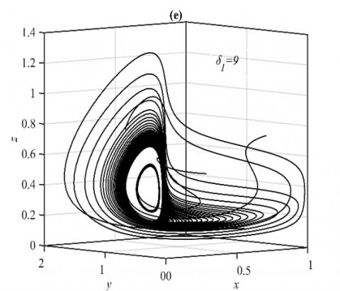
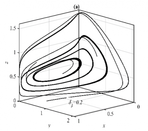
It should be observed that, as illustrated in Figure 1 below, the system (3) approaches the CEEP under set (36) asymptotically. Moreover, the influence of the varying parameter δ1 on the system (3)’s dynamic in the ranges $\delta_1 \in[0,4), \delta_1 \in[4,9)$, and δ1≥9 is explored as an asymptotic stable at E5, approaches to 3D periodic dynamics, and approaches to multiple 3D periodic that are in the form of nonlinear center respectively, see Figure 1 for selected values.
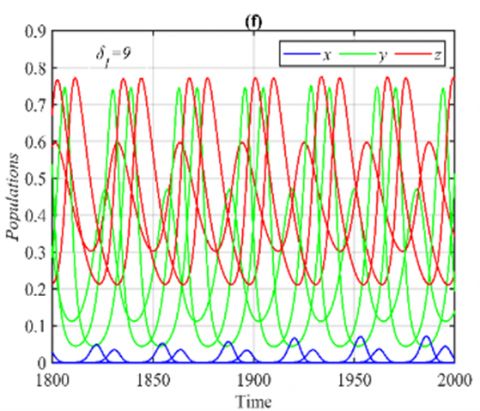
For the parameter δ2 in the range $\delta_2 \in(0,1)$, it is obtained that the system has a G.A.S. E5 with small quantitative changes in the population size. However, when the system approaches 3D periodic dynamics, such as the case in Figure 1(c)-(d), it is observed that shrink the periodic to a stable point as shown in Figure 2.
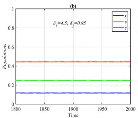
For the ranges $\delta_3 \in(0,0.23]$ and $\delta_3 \in(0.23,1)$, it has been shown that the system (3) approaches asymptotically to multiple periodic dynamics (nonlinear center) and E5 respectively as explained in Figure 3.
When the parameter δ4 goes within the ranges $\delta_4 \in(0,0.18]$ and $\delta_4 \in(0.18,1)$, respectively, the system approaches various multiple periodic attractors and E5, while maintaining the other parameters as in the set (36), see Figure 4 for some selected values of δ4.
Figure 1. The trajectories of system (3) using the set (40) with different initial points: (a) Phase portrait that approaches to E5=(0.56,0.25,0.46); (b) The time series for the trajectories in (a); (c) Phase portrait when δ1=4.5 that approaches to 3D periodic attractor with different phase angles; (d) The time series when δ1=4.5; (e) Two different 3D periodic attractors when δ1=9; (f) The time series for δ1=9
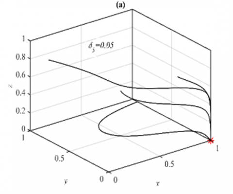
Figure 2. Time series of the system (3) using the set (40) with different initial points and δ1=4.5, δ2=0.95. (a) Complete range of time series in which the system approaches to E5=(0.11,0.24,0.44); (b) Part of the time series to compare it with that given in Figure (1d)
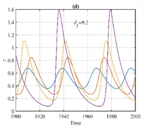
Figure 3. The trajectories of system (3) using the set (40) with different initial points: (a) Phase portrait that approaches four different periodic attractors when δ3=0.2; (b) Time series when δ3=0.2 for trajectories of x; (c) Time series when δ3=0.2 for trajectories of y; (d) Time series when δ3=0.2 for trajectories of z; (e) Phase portrait when δ3=0.5 that approaches to E5=(0.62,0.25,0.35); (f) The time series when δ3=0.5
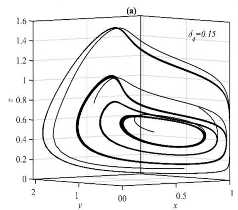
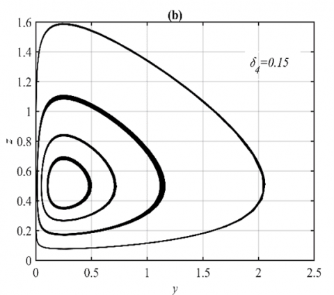
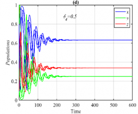
Figure 4. The trajectories of system (3) using the set (40) with different initial points: (a) Phase portrait that approaches four different periodic attractors when δ4=0.15; (b) Projection of phase portrait on the yz-plane; (c) Phase portrait when δ4=0.5 that approaches to E5=(0.63,0.25,0.33); (d) The time series when δ4=0.5
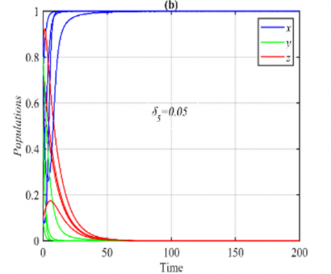
Figure 5. The trajectories of system (3) using the set (40) with different initial points: (a) Phase portrait when δ5=0.05 that approaches to E1=(1,0,0); (b) The time series when δ5=0.05
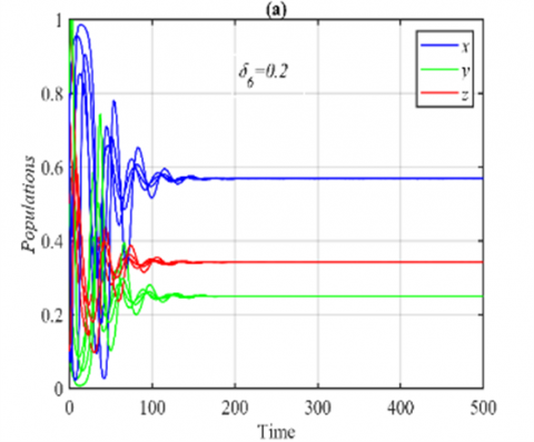
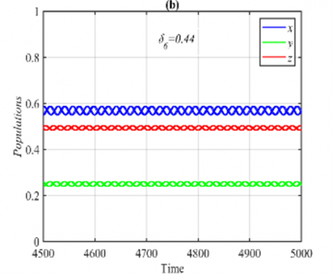
Figure 6. Time series of the system (3) using the set (40) with different initial points: (a) Time series when δ6=0.2 in which the system approaches to E5=(0.56,0.25,0.34); (b) The final state of the time series when δ6=0.44 in which the system approaches the same periodic attractor with different phase angles
Figure 7. Time series of the system (3) using the set (40) with different initial points: (a) Time series when δ7=0.2 in which the system approaches to E5=(0.56,0.25,0.36); (b) Time series when δ7=0.57 in which the system approaches to E3=(0.61,0.22,0); (c) Time series when δ7=0.6 in which the system approaches to E1=(1,0,0)
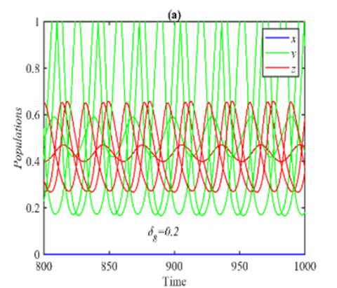
Figure 8. The trajectories of system (3) using the set (40) with different initial points: (a) Final state Time series when δ8=0.2 in which the system approaches two different periodic attractors in the yz-plane; (b) The projection of the trajectories on the yz-plane when δ8=0.2
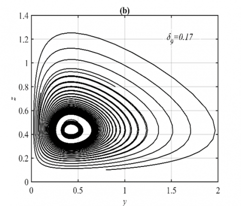
Figure 9. The trajectories of system (3) using the set (40) with different initial points: (a) Final state of the time series when δ9=0.17 in which the system approaches two different periodic attractors in the yz-plane; (b) The projection of the trajectories on the yz-plane when δ9=0.17
The parameters δ3 and δ4 have similar effects on the dynamic behavior of the system (3). Now, for the ranges $\delta_5 \in(0,0.1]$ and $\delta_5 \in(0.1,1)$, it is obtained that the solution of system (3) approaches E1 and E5 respectively, see Figure 5 for the typical value in the first range and Figure 1(a) for the second range.
On the other hand, for the ranges $\delta_6 \in(0,0.43]$ and δ6>0.43, it is obtained that the solution of system (3) approaches E5 and 3D periodic attractor respectively, see Figure 6 for the typical values of δ6.
It is observed that the system (3) approaches E5, E3, and E1 when δ7 falls in the ranges $\delta_7 \in(0,0.56], \quad \delta_7 \in(0.56,0,58), \quad$ and $\quad \delta_7 \in[0.58,1]$ respectively, as shown in Figure 7 for the selected values of δ7.
However, for the ranges $\delta_8 \in(0,0.24]$ and $\delta_8 \in(0.24,1]$ the system (3) approaches asymptotically multiple periodic attractors in the yz-plane and E5 respectively, see Figure 8 for the selected value of δ8 in the first range and Figure 1(a) for the second range. Finally, the system (3) approaches asymptotically E5 and multiple periodic attractors in the yz-plane when $\delta_9 \in(0,0.15]$ and $\delta_9 \in(0.15,1]$ respectively, see for example Figure 9 for the selected value of δ9.
This work develops a mathematical model of a prey-predator system with an infectious sickness in the predator. The dynamics of this system have been examined about fear, shelter that is dependent on predators, and increased food. Different mathematical techniques, including linearization, Lyapunov functions, and the Local Bifurcation Theorem, are used to conceptually study the system. It is obtained that it contains six nonnegative equilibrium points in all. Following the determination of each of their existence criteria, the local stability and bifurcation around each of them are investigated. When it is feasible, the Lyapunov function is used to investigate global stability. Finally, the system is numerically solved using a fictitious set of data to comprehend the results and identify how the parameters affect the dynamical behavior of the system.
It is common knowledge that equilibrium points, or stable points in ecological models, reflect the steady states or dynamics of an ecological system. They display the locations where populations are steady over time. Understanding the flexibility, stability, and variety of ecosystems depends on these stable points. Ecologists can learn more about the mechanisms and processes that control species interactions, population dynamics, and the general health of ecosystems by locating and examining stable spots. However, stable points are frequently used to exhibit endemic or disease-free equilibrium states in epidemiological models. Whereas endemic equilibrium exhibits a stable state in which the disease remains to exist in a community at a consistent level, disease-free equilibrium indicates a stable state in which the disease is missing. understanding the dynamics of infectious diseases, including their spread, persistence, and decline within a community, necessitates an understanding of these stable spots. Stable points are used by epidemiologists to check up on a range of variables that impact the spread of disease, including treatment, immunization, population density, and behavioral shifts. To effectively treat ecological and epidemiological systems, stable points are fundamental. Knowledge of stable points in ecological systems can be useful in locating tipping points, important thresholds, and possible ecosystem transitions. With this knowledge, policymakers and environmentalists may put into experience suitable methods for habitat restoration, biodiversity conservation, and sustainable resource management. Stable points are useful in epidemiology because they help with illness outcome prediction, intervention strategy evaluation, and control measure design. Public health professionals can carry out focused actions to stop disease outbreaks or lower disease burdens by considering stability points.
In contrast to the above case, Oscillatory patterns in several species or the number of people suffering from an illness might result from periodic dynamics. Seasonal alterations, predator-prey relationships, and other factors can lead to these oscillations. It's critical to understand these patterns to forecast and control population dynamics and disease outbreaks. Moreover, environments and communities can be turned more resilient and stable via periodic dynamics. Periodic fluctuations in ecological systems can be a sign of a supply of nutrients cycle or a predator-prey system that is in equilibrium, both of which support the ecosystem's overall stability. On the other hand, strong or unpredictable oscillations may cause instability and even a breakdown of an ecosystem. Similar to this, periodic patterns in epidemiological systems could suggest fluctuations in the spread of disease, helping in evaluating the necessary resilience and control measures.
Finally, for ecological and epidemiological models to be managed and controlled successfully, bifurcation must be understood and expected. Scientists and governments can create plans to maintain ecological balance, stop the decline of biodiversity, and engage in immediate actions to contain and lessen disease outbreaks by identifying the factors and circumstances that cause bifurcations.
Based on the above, our study has shown the following results, which reflect the influence of parameters and their change on the behavior of the proposed system. It is observed that, the proposed system has both periodic and nonlinear centers (multiple periodic) attractors. Based on how they affect the system's dynamic behavior, the parameters are separated into two groups. The predator-dependent refuge level, half saturation constant, additional food constant, conversion rate, and incidence rate make up the first compartment that stabilizes the dynamics of the system. The amount of anxiety, the rate at which additional food sources are converted, and the rate at which infected predators die, including those that die from the disease, make up the second compartment, which has a detrimental impact on the dynamic behavior of the system (3) (destabilizing the system). Finally, the death rate of the susceptible predator causes ultimately extrication of the predator species.
|
r |
The prey's intrinsic growth rate |
|
a |
Intraspecific competition |
|
n |
Fear level |
|
b |
The prey predation rate by a susceptible predator |
|
c |
The predator half-saturation constant |
|
u |
Represents the capturing time ratio of additional food to prey |
|
v |
Represents the constant dependent ratio for the movement rate of populations concerning the additional food |
|
e |
The conversion rate |
|
m |
The prey refuge rate |
|
k |
The infection rate of predator |
|
d1, d2 |
The death rates of the susceptible and infected predators respectively |
|
A |
The additional food |
[1] Anderson, R.M., May, R.M. (1981). The population dynamics of microparasites and their invertebrate hosts. Philosophical Transactions of the Royal Society of London. Series B, Biological Sciences, 291(1054): 451-524. https://doi.org/10.1098/rstb.1981.0005
[2] Anderson, R.M., May, R.M. (1986). The invasion, persistence and spread of infectious diseases within animal and plant communities. Philosophical Transactions of the Royal Society of London. Series B, Biological Sciences, 314(1167): 533-570. https://doi.org/10.1098/rstb.1986.0072
[3] Hadeler, K.P., Freedman, H.I. (1989). Predator-prey populations with parasitic infection. Journal of Mathematical Biology, 27(6): 609-631. https://doi.org/10.1007/BF00276947
[4] Chattopadhyay, J., Arino, O. (1999). A predator-prey model with disease in the prey. Nonlinear Analysis, 36: 747-766. http://doi.org/10.1016/S0362-546X(98)00126-6
[5] Sharma, S., Samanta, G.P. (2015). A ratio-dependent predator-prey model with Allee effect and disease in prey. Journal of Applied Mathematics and Computing, 47: 345-364. https://doi.org/10.1007/s12190- 014-0779-0
[6] Saifuddin, M., Samanta, S., Biswas, S., Chattopadhyay, J. (2017). An eco-epidemiological model with different competition coefficients and strong-Allee in the prey. International Journal of Bifurcation and Chaos, 27(8): 1730027. https://doi.org/10.1142/s0218127417300270
[7] Abdulghafour, A.S., Naji, R.K. (2018). A study of a diseased prey-predator model with refuge in prey and harvesting from predator. Journal of Applied Mathematics, 2018(1): 2952791. https://doi.org/10.1155/2018/2952791
[8] Ibrahim, H.A., Naji, R.K. (2020). A prey-predator model with Michael Mentence type of predator harvesting and infectious disease in prey. Iraqi Journal of Science, 1146-1163. https://doi.org/10.24996/ijs.2020.61.5.23
[9] Melese, D., Muhye, O., Sahu, S.K. (2020). Dynamical behavior of an eco-epidemiological model incorporating prey refuge and prey harvesting. Applications and Applied Mathematics: An International Journal (AAM), 15(2): 28. https://digitalcommons.pvamu.edu/aam/vol15/iss2/28.
[10] Hossain, M., Pal, N., Samanta, S. (2020). Impact of fear on an eco-epidemiological model. Chaos, Solitons & Fractals, 134: 109718. https://doi.org/10.1016/j.chaos.2020.109718
[11] Ashwin, A., Sivabalan, M., Divya, A. (2023). Dynamics of Holling type II eco-epidemiological model with fear effect, prey refuge, and prey harvesting. In the 1st International Online Conference on Mathematics and Applications Session Mathematical Biology. https://doi.org/10.3390/IOCMA2023-14404
[12] Haque, M. (2010). A predator–prey model with disease in the predator species only. Nonlinear Analysis: Real World Applications, 11(4): 2224-2236. https://doi.org/10.1016/J.NONRWA.2009.06.012
[13] Das, K.P. (2011). A mathematical study of a predator-prey dynamics with disease in predator. International Scholarly Research Notices, 2011(1): 807486. https://doi.org/10.5402/2011/807486
[14] Pal, P.J., Haque, M., Mandal, P.K. (2014). Dynamics of a predator–prey model with disease in the predator. Mathematical Methods in the Applied Sciences, 37(16): 2429-2450. https://doi.org/10.1002/mma.2988
[15] Mbava, W., Mugisha, J.Y.T., Gonsalves, J.W. (2017). Prey, predator and super-predator model with disease in the super-predator. Applied Mathematics and Computation, 297: 92-114. https://doi.org/10.1016/j.amc.2016.10.034
[16] Mondal, A., Pal, A.K., Samanta, G.P. (2019). On the dynamics of evolutionary Leslie-Gower predator-prey eco-epidemiological model with disease in predator. Ecological Genetics and Genomics, 10: 100034. https://doi.org/10.1016/j.egg.2018.11.002
[17] Satar, H.A., Ibrahim, H.A., Bahlool, D.K. (2021). On the dynamics of an eco-epidemiological system incorporating a vertically transmitted infectious disease. Iraqi Journal of Science, 1642-1658. https://doi.org/10.24996/ijs.2021.62.5.27
[18] Hsieh, Y.H., Hsiao, C.K. (2008). Predator–prey model with disease infection in both populations. Mathematical Medicine and Biology: A Journal of the IMA, 25(3): 247-266. http://doi.org/10.1093/imammb/dqn017
[19] pada Das, K., Kundu, K., Chattopadhyay, J. (2011). A predator–prey mathematical model with both the populations affected by diseases. Ecological Complexity, 8(1): 68-80. https://doi.org/10.1016/j.ecocom.2010.04.001
[20] Bera, S.P., Maiti, A., Samanta, G.P. (2015). A prey-predator model with infection in both prey and predator. Filomat, 29(8): 1753-1767. https://doi.org/10.2298/FIL1508753B
[21] Bezabih, A.F., Edessa, G.K., Rao, K.P. (2021). Ecoepidemiological model and analysis of prey-predator system. Journal of Applied Mathematics, 2021(1): 6679686. https://doi.org/10.1155/2021/6679686
[22] Arditi, R., Ginzburg, L.R. (1989). Coupling in predator-prey dynamics: Ratio-Dependence. Journal of Theoretical Biology, 139(3): 311-326. https://doi.org/10.1016/s0022-5193(89)80211-5
[23] Abdul Satar, H., Naji, R.K. (2019). Stability and bifurcation of a prey-predator-scavenger model in the existence of toxicant and harvesting. International Journal of Mathematics and Mathematical Sciences, 2019(1): 1573516. https://doi.org/10.1155/2019/1573516
[24] Majeed, S.J., Naji, R.K., Thirthar, A.A. (2019). The dynamics of an Omnivore-predator-prey model with harvesting and two different nonlinear functional responses. AIP Conference Proceedings, 2096: 020008. https://doi.org/10.1063/1.5097805
[25] Satar, H.A., Naji, R.K. (2022). Stability and bifurcation in a prey–predator–scavenger system with Michaelis–Menten type of harvesting function. Differential Equations and Dynamical Systems, 30(4): 933-956. https://doi.org/10.1007/s12591-018-00449-5
[26] Al-Momen, S., Naji, R.K. (2022). The dynamics of modified Leslie Gower predator-prey model under the influence of nonlinear harvesting and fear effect. Iraqi Journal of Science, 63(1): 259-282. https://doi.org/10.24996/ijs.2022.63.1.27
[27] Rayungsari, M., Suryanto, A., Kusumawinahyu, W.M., Darti, I. (2023). Dynamics analysis of a predator–prey fractional-order model incorporating predator cannibalism and refuge. Frontiers in Applied Mathematics and Statistics, 9: 1122330. https://doi.org/10.3389/fams.2023.1122330
[28] Naji, R.K. (2023). Contribution of hunting cooperation and antipredator behavior to the dynamics of the harvested prey-predator system. Communications in Mathematical Biology and Neuroscience, 2023: 99. http://doi.org/10.28919/cmbn/8164
[29] Wang, X., Zanette, L., Zou, X. (2016). Modelling the fear effect in predator–prey interactions. Journal of Mathematical Biology, 73(5): 1179-1204. https://doi.org/10.1007/S00285-016-0989-1
[30] Panday, P., Pal, N., Samanta, S., Chattopadhyay, J. (2018). Stability and bifurcation analysis of a three-species food chain model with fear. International Journal of Bifurcation and Chaos, 28(1): 1850009. https://doi.org/10.1142/S0218127418500098
[31] Fakhry, N.H., Naji, R.K. (2020). The dynamics of a square root prey-predator model with fear. Iraqi Journal of Science, 61(1): 139-146. https://doi.org/10.24996/ijs.2020.61.1.15
[32] Maghool, F.H., Naji, R.K. (2021). The dynamics of a Tritrophic Leslie-Gower food‐web system with the effect of fear. Journal of Applied Mathematics, 2021(1): 2112814. https://doi.org/10.1155/2021/2112814
[33] Jamil, A.R.M., Naji, R.K. (2022). Modeling and analysis of the influence of fear on the harvested modified Leslie–Gower model involving nonlinear prey refuge. Mathematics, 10(16): 2857. https://doi.org/10.3390/math10162857
[34] Nadim, S.S., Samanta, S., Pal, N., ELmojtaba, I.M., Mukhopadhyay, I., Chattopadhyay, J. (2018). Impact of predator signals on the stability of a Predator–Prey System: A Z-control approach. Differential Equations and Dynamical Systems, 30: 451-467. https://doi.org/10.1007/S12591-018-0430-X
[35] Abbas, Z.S., Naji, R.K. (2022). Modeling and analysis of the influence of fear on a harvested food web system. Mathematics, 10(18): 3300. https://doi.org/10.3390/MATH10183300
[36] González-Olivares, E., Ramos-Jiliberto, R. (2003). Dynamic consequences of prey refuges in a simple model system: More prey, fewer predators and enhanced stability. Ecological Modelling, 166(1-2): 135-146. https://doi.org/10.1016/S0304-3800(03)00131-5
[37] Smith, J. (1978). Models in Ecology Excerpts. First edition, London: Cambridge University Press. https://books.google.iq/books/about/Models_in_Ecology.html?id=Jgk4AAAAIAAJ&redir_esc=y.
[38] Sih, A. (1987). Prey refuges and predator-prey stability. Theoretical Population Biology, 31(1): 1-12. https://doi.org/10.1016/0040-5809(87)90019-0
[39] Yu, X., Sun, F. (2013). Global dynamics of a predator-prey model incorporating a constant prey refuge. Electronic Journal of Differential Equations, 2013(4): 1-8. https://ejde.math.txstate.edu/Volumes/2013/04/yu.pdf.
[40] Das, U., Kar, T.K., Pahari, U.K. (2013). Global dynamics of an exploited prey-predator model with constant prey refuge. International Scholarly Research Notices, 2013(1): 637640. https://doi.org/10.1155/2013/637640
[41] Kar, T.K. (2005). Stability analysis of a prey–predator model incorporating a prey refuge. Communications in Nonlinear Science and Numerical Simulation, 10(6): 681-691. https://doi.org/10.1016/J.CNSNS.2003.08.006
[42] Chakraborty, B., Bairagi, N. (2019). Complexity in a prey-predator model with prey refuge and diffusion. Ecological Complexity, 37: 11-23. https://doi.org/10.1016/J.ECOCOM.2018.10.004
[43] Das, A., Samanta, G.P. (2020). A prey–predator model with refuge for prey and additional food for predator in a fluctuating environment. Physica A: Statistical Mechanics and its Applications, 538: 122844. https://doi.org/10.1016/J.PHYSA.2019.122844
[44] Zhao, J., Shao, Y. (2023). Bifurcations of a prey-predator system with fear, refuge and additional food. Mathematical Biosciences and Engineering, 20(2): 3700-3720. https://doi.org/10.3934/mbe.2023173
[45] Surendar, M.S., Sambath, M., Balachandran, K., Ma, Y.K. (2023). Qualitative analysis of a prey–predator model with prey refuge and intraspecific competition among predators. Boundary Value Problems, 2023(1): 81. https://doi.org/10.1186/s13661-023-01771-w
[46] Jang, S.R., Yousef, A.M. (2023). Effects of prey refuge and predator cooperation on a predator–prey system. Journal of Biological Dynamics, 17(1): 2242372. https://doi.org/10.1080/17513758.2023.2242372
[47] Pal, S., Al Basir, F., Ray, S. (2023). Impact of cooperation and intra-specific competition of prey on the stability of prey–predator models with refuge. Mathematical and Computational Applications, 28(4): 88. https://doi.org/10.3390/mca28040088
[48] Rahman, M.S., Islam, M.S., Sarwardi, S. (2023). Effects of prey refuge with Holling type IV functional response dependent prey predator model. International Journal of Modelling and Simulation, 1-19. https://doi.org/10.1080/02286203.2023.2178066
[49] Mondal, B., Sarkar, A., Sk, N. (2023). Treatment of infected predators under the influence of fear-induced refuge. Scientific Reports, 13(1): 16623. https://doi.org/10.1038/s41598-023-43021-0
[50] Manarul Haque, M., Sarwardi, S. (2018). Dynamics of a harvested prey–predator model with prey refuge dependent on both species. International Journal of Bifurcation and Chaos, 28(12): 1830040. https://doi.org/10.1142/S0218127418300409
[51] Mondal, S., Samanta, G.P. (2019). Dynamics of an additional food provided predator–prey system with prey refuge dependent on both species and constant harvest in predator. Physica A: Statistical Mechanics and Its Applications, 534: 122301. https://doi.org/10.1016/J.PHYSA.2019.122301
[52] Jabr, E.A.A.H., Bahlool, D.K. (2021). The dynamics of a food web system: Role of a prey refuge depending on both species. Iraqi Journal of Science. 62(2): 639-657. https://doi.org/10.24996/ijs.2021.62.2.29
[53] Ibrahim, H.A., Bahlool, D.K., Satar, H.A., Naji, R.K. (2022). Stability and bifurcation of a prey-predator system incorporating fear and refuge. Communications in Mathematical Biology and Neuroscience, 2022: 32. http://doi.org/10.28919/cmbn/7260
[54] Vinoth, S., Vadivel, R., Hu, N.T., Chen, C.S., Gunasekaran, N. (2023). Bifurcation analysis in a harvested modified Leslie–Gower model incorporated with the fear factor and prey refuge. Mathematics, 11(14): 3118. https://doi.org/10.3390/math11143118
[55] Perko, L. (2001). Differential Equations and Dynamical Systems. Springer, New York, 3rd edition. http://doi.org/10.1007/978-1-4613-0003-8